Statistical analysis of ionospheric vertical total electron content anomalies before global Mw≥6.0 shallow earthquakes during 2000–2020

To quantitatively investigate the relationship between earthquakes and ionospheric anomalies, this paper presents a statistical study of pre-earthquake vertical total electron content (VTEC) variations. A total of 1522 shallow (≤60 km) strong (Mw≥6.0) earthquakes in the global area during 2000-2020 are selected, and classified according to different magnitudes, latitudes and focal depths. A quartile-based process with different lengths of sliding windows, equaling 10 days, 15 days and 27 days, respectively, has been utilized to detect VTEC anomalies. The abnormal level is first defined, and then VTEC anomalies occurrence probabilities ($P_o$) and occurrence rates ($P_E$) within 1-10 days before 1522 earthquakes have been calculated. Besides, VTEC anomalies occurrence rates of the background days (PN) are also calculated. The results show that the significant correlation between Po and epicentral latitudinal locations could be observed within 1-10 days before earthquakes. The values of Po increase with larger magnitudes in the equatorial and low-latitude regions, but decrease with greater magnitudes in the mid- and high-latitude regions to some degree. Within 1-5 days before earthquakes, the overall trend of $P_E$ shows an increase with larger magnitudes, but the correlation between the values of $P_E$ and magnitudes is relatively weak in the southern mid- and high-latitude regions. There is no evident causality between PN and the magnitude, and most of the values of $P_E/P_N$ are larger than 1, indicating that VTEC anomalies within a few days before earthquakes are probably related with the forthcoming earthquakes. Moreover, when the abnormal level exceeds 60%, different sliding window lengths have a significant impact on the values of $P_o$ and $P_E$ in the mid- and high-latitude regions. In particular, there are obvious systematic deviations between the values of $P_o$ obtained from different sliding windows in the southern mid- and high-latitude regions. However, the selection of the optimal sliding window needs to be further studied.

1 Introduction

The seismic process is not only confined to the lithosphere, but also has impacts on the troposphere, ionosphere and even magnetosphere through the electromagnetic fields effect. The ionospheric anomalies within a few days before the earthquakes are relatively stable at short time scales, and have been studied widely in the field of earthquake prediction (Pulinets and Boyarchuk, 2004; Liperovsky et al., 2008; Pulinets and Ouzounov, 2011). A large number of studies have shown that ionospheric perturbations before many earthquakes could be identified (e.g., Liu et al., 2001; Le et al., 2011; Zhu et al., 2014; Tang et al., 2015; Sun et al., 2016; Parrot and Li, 2018; Pulinets et al., 2021). The possible earthquake-related NmF2 (F2 layer peak electron density) and TEC anomalies have been widely discussed in recent decades (e.g., Nishihashi et al., 2009; Ma et al., 2014). Especially, because of the development of the Global Navigation Satellite system (GNSS), GNSS VTEC have attracted more and more attention in the investigation of the ionospheric variations prior to large earthquakes (Liu et al., 2004; Shah and Jin, 2015). For the first time, Liu et al. (2001) used GNSS(GPS) VTEC to study the ionospheric disturbance before the Chi-Chi earthquake, and found that the VTEC over the epicenter decreased significantly 1, 3 and 4 days before the earthquake. Later on, more and more scientists began to focus on GNSS VTEC variations before earthquakes, aiming to detect the potential ionospheric anomalies related to the forthcoming earthquakes. For example, Yao et al. (2012) analyzed ionospheric variations prior to the 2011 Mw9.0 Japan earthquake, and indicated that ionospheric anomalies occurring on 8 March might be a precursor of the earthquake; Ho et al. (2013) showed that TEC increased 9–19 days before the 2010 M8.8 Chile earthquake and specifically over the epicenter; Su et al. (2013) investigated ionospheric TEC variations before the Hector Mine earthquake, and found that ionospheric disturbance appeared just above the epicenter 5 days before the earthquake. These studies show that the GNSS TEC anomalies appear a few days before the earthquake with different magnitude and focal depth.

Over about 50 years of research, no consensus in the scientific community has been formed on the existence of ionospheric earthquake precursors (Rishbeth, 2006; Dautermann et al., 2007; Masci, 2012; Ovalle et al., 2013; Masci and Thomas, 2014; Zolotov et al., 2019). Dautermann et al. (2007) indicated that there was no statistically significant correlation between TEC anomalies and earthquakes in Southern California during 2003–2004; Kon et al. (2011) selected M≥6.0 earthquakes in Japan during 1998–2010, and found that significant positive TEC anomalies within 1000 km above the epicenter appeared within 1–5 days before the earthquakes. According to Masci (2012), the analysis of Kon et al. (2011) was not reliable because of the influence of global geomagnetic events. Ovalle et al. (2013) concluded that it remained controversial whether the observed NmF2 and TEC anomalies were unambiguously related to the 2010 M8.8 Chile earthquake. Background geomagnetic events may impact revealing the relationship between TEC anomalies and earthquakes.

To validate the relationship between ionospheric anomalies and earthquakes in response to the controversy, many scientists have undertaken a multitude of studies on the physical mechanism of generating ionospheric anomalies. Firstly, the morphological characteristics of ionospheric anomalies before a large number of earthquakes are summarized. For instance, Liu et al. (2004) analyzed Ms5.0+ earthquakes in Taiwan from 1999 to 2002, and found that obvious negative TEC anomalies occurred 5 days before the earthquakes. Le et al. (2011) made a statistical study of global 736 M≥6.0 earthquakes during 2002–2010, and proposed that occurrence rates of abnormal days are larger for earthquakes with greater magnitude and lower depth. De Santis et al. (2019) analyzed the electron density and magnetic field data from 3 Swarm satellites to detect possible anomalies associated with 1312 M≥5.5 shallow earthquakes from January 2014 to August 2018, and the results showed that anomalies occurred between a few days and 80 days before the earthquakes with larger peaks at around 10, 20 and 80 days, and supported the Lithosphere-Atmosphere-Ionosphere Coupling (LAIC) with clear statistical significance. Shah et al. (2020) studied the ionospheric anomalies before the global Mw≥5.0 earthquakes from 1998 to 2019, and the results revealed that prominent ionospheric anomalies appeared within 5 days before and after the earthquakes. Based on the characteristics of ionospheric anomalies prior to a large number of earthquakes, the physical mechanisms of seismic LAIC have been extensively studied (Freund, 2011; Klimenko et al., 2012; Pulinets, 2012; Zolotov et al., 2012). For example, Freund (2011) proposed that positive holes released by stressed rocks are highly mobile and can reach the Earth’s surface, and then ionize the atmosphere and change the vertical electric field between the ground and the lower edge of the ionosphere. In addition, a large number of studies have shown that anomalous atmospheric electric field variations in the earthquake preparation zone are likely to be the main cause of ionospheric disturbance (Zhang et al., 2014; Jiang et al., 2017; Pulinets and Davidenko, 2018; Davidenko and Pulinets, 2019). For example, Namgaladze et al. (2009) proposed that vertical plasma motion in the ionospheric F2 region under the action of the zonal electric field is the main disturbance formation factor, and ionospheric anomalies before strong earthquakes at middle and low latitudes verified this mechanism. Liu et al. (2010) studied the crest of equatorial ionization anomaly (EIA) variations before 150 M≥5.0 earthquakes in Taiwan, and the results implied that the weak atmospheric electric field a few days before the earthquakes may cause the EIA crest anomalies.

Both the characteristics of ionospheric anomalies and the physical mechanisms of lithosphere-atmosphere-ionosphere coupling present diversity and complexity, and the influence factors may include magnitudes, focal depths, latitude and longitude of the epicenter, focal mechanisms, the weather, the season, solar and geomagnetic activity and so on. However, many studies focused on a single large earthquake, and there are relatively few statistical results based on a large number of earthquakes. The corresponding characteristics of the ionospheric anomalies are still not fully understood. In addition, a quartile-based process is the most common method for extracting ionospheric VTEC anomalies, but different authors use different numbers of days as the lengths of the sliding windows, such as, 10 days (e.g., Zhou et al., 2009; Zhu et al., 2014), 15 days (e.g., Liu et al., 2010; Ke et al., 2016; Liu and Xu, 2017), 27 days (e.g., Xu et al., 2011; Guo et al., 2015), etc. It should be noted that the effects of different sliding windows on the ionospheric anomalies are rarely studied (Zolotov et al., 2019). To solve the above problems, this study uses GIM VTEC to carry out a statistical analysis by studying the VTEC anomalies within 1–10 days before 1522 global shallow (≤60 km) Mw≥6.0 earthquakes during 2000–2020. The factors, including the magnitude, focal depth and the latitude of the epicenter are considered for all the earthquakes, and the effects of different sliding windows on ionospheric anomalies are investigated. Moreover, ionospheric anomalies during background days are also analyzed to compare with those prior to the earthquakes. This study aims at helping the research on the physical mechanisms of lithosphere-atmosphere-ionosphere coupling by summarizing the characteristics of ionospheric anomalies comprehensively, and determining whether different lengths of sliding windows affect ionospheric anomalies features.

2 Data and method

2.1 Data source

The worldwide Mw≥6.0 earthquakes during 2000–2020 are selected to analyze ionospheric anomalies in this study. The data are retrieved from the Global Centroid Moment Tensor (CMT) Project (http://www.globalcmt.org/). The earthquakes selected in this study are declustered from aftershocks following the method of Michael (2011), and the earthquakes occurring at the similar location but with the short interval (<10 days) from the previous ones are also excluded to avoid possible confounded effects from adjacent earthquakes. Finally, 1522 shallow (≤60 km) earthquakes are selected, and Figure 1 illustrates epicenter locations of these earthquakes.

FIGURE 1

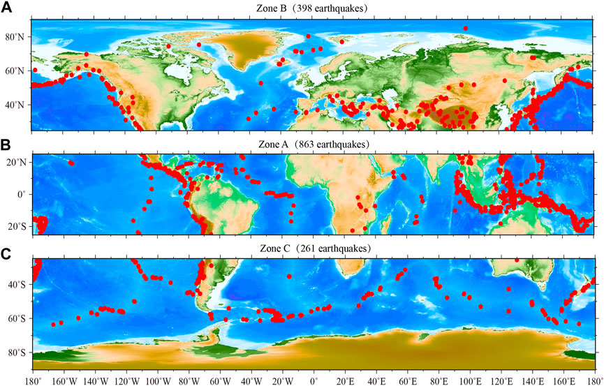
FIGURE 1. Locations of global 1522 Mw≥6.0 earthquakes during 2000–2020.

The GIM VTEC is derived using the observations from hundreds of global GNSS stations (Hernández-Pajares et al., 2009). The GIM covers $\pm 87.5^{\circ }$ latitude and $\pm {180}^{\circ }$ longitude ranges with spatial resolutions of $2.5^{\circ }$ and $5^{\circ }$, respectively, and the time interval of the VTEC is 2 h. For each earthquake, the cell including the epicenter was selected as the point to analyze ionospheric VTEC anomalies. According to Dobrovolsky, (1979), the radius of the M6.0 earthquake preparation zone is about 380 km, corresponding to $3.5^{\circ }$. Therefore, the spatial resolution of GIM VTEC is sufficient to extract ionospheric anomalies using the nearest grid to the epicenter.

The equatorial geomagnetic activity index (Dst) data provided by the World Data Center for Geomagnetism, Kyoto (https://wdc.kugi.kyoto-u.ac.jp/) are used to represent the geomagnetic activity.

2.2 Statistical method

In this study, a quartile-based process is performed to detect ionospheric VTEC anomalies within 1–10 days prior to each earthquake. As the length of sliding window is limited by the seasonal variability of the ionosphere at longer timescales, 10, 15, and 27 days are chosen as the candidate lengths of sliding windows based on the previous studies. At each time point on any day, the median $\overline{x}$ is computed using the VTEC at the same time point within 10, 15, and 27 days before this day as the background value, respectively, and the associated inter-quartile range $IQR$ is also obtained to construct the upper or lower bound $\overline{x}\pm 1.5IQR$. If VTEC continuously exceeds the associated upper or lower bounds for at least 6 h during a day, this day would be considered as an anomalous day. Moreover, the abnormal level (AL) is defined as the percentage of the largest deviation from the median (Le et al., 2011). Ionospheric anomalies with AL<20% are regarded as the daily effects of solar activities (Le et al., 2011, Personal Communication), therefore, only ionospheric anomalies with AL>20% are analyzed in this study. In addition, the ionospheric anomalies with AL>40% and AL>60% (i.e., $n\times AL,n=\mathrm{1,2,3}$ with $AL=20\%$) are also checked for the purpose of studying whether the characteristics of ionospheric anomalies are similar with different AL. If a day with Dst≤−40 nT or Dst≥40nT, this day and the following 3 days are excluded to avoid the interference of the magnetic disturbed activity. After removing the effects of daily solar activity and geomagnetic disturbance, ionospheric anomalies occurring on 1 day are recorded as the seismo-ionospheric anomalies.

After the analysis of seismo-ionospheric anomalies for each event, 1522 earthquakes are divided into three different latitudinal zones (as shown in Figure 1), and VTEC anomalies occurrence probabilities ($P_o$) and occurrence rates ($P_E$) will be investigated respectively. For each zone, the earthquakes are firstly classified by magnitudes in increments of 0.1 or by depths in increments of 20km, and then we calculate $P_o$ and $P_E$ of each group. $P_o$ can be computed as the ratio of the number of earthquakes with seismo-ionospheric anomalies and the total number of earthquakes (Fujiwara et al., 2004), as shown in Eq. 1. In this equation, $N{o}_{AL}$ and $N{o}_{Total}$ are the number of earthquakes with seismo-ionospheric anomalies and the total number of all the earthquakes in each group, respectively. For example, in the group (Mw ≥ 6.5 in Zone A with AL>20%), $P_o$ is the number of earthquakes with seismo-ionospheric anomalies divided by the total number of earthquakes.

$P_o=\frac{N{o}_{AL}}{N{o}_{Total}}(1)$

The occurrence rates for the $n$ th earthquake $P_{En}$ can be calculated as the ratio of the number of the seismo-ionospheric abnormal days and the total quiet days: $N_{AL,T}^n/\left(T-\Delta S_n\right)$, and $P_E$ is defined as the mean of $P_{En}$, as shown in Eq. 2, derived from Le et al. (2011). In this equation, $K$ is the number of earthquakes in each group (for example, Mw ≥ 6.5 in Zone A with AL>20%); $N_{AL,T}^n$ is the number of seismo-ionospheric days with different AL (for example, AL>20%) within the $T$ days before the $n$ th earthquake, and $T=\mathrm{1,2,3},...,10$; $\Delta S_n$ is the number of magnetic disturbed days during the 1–10 days before the $n$ th earthquake; $N_{AL,T}^n/\left(T-\Delta S_n\right)$ is the number of the seismo-ionospheric abnormal days divided by the number of the total quiet days before the $n$ th earthquake.

$PE=\frac{1}{K}{\displaystyle \sum _{n=1}^K}\frac{N_{AL,T}^n}{T-\Delta S_n}\times 100\%(2)$

3 Results and discussions

3.1 Seismo-ionospheric anomalies occurrence probabilities

According to the method described above, we calculated $P_o$ for earthquakes with different magnitudes and depths. Figure 2 shows $P_o$ with AL > 20%, 40%, and 60% within 1–10 days before different magnitude earthquakes with the depth ≤20, ≤40, and ≤60 km, respectively. It can be seen from Figure 2 (left), there is no significant correlation between the values of $P_o$ and the magnitude for the earthquakes of 6.0≤Mw < 6.5 in all three zones. There are larger values of $P_o$ in Zone A for larger magnitude earthquakes of Mw≥6.5, but the values of $P_o$ decrease with the magnitudes increasing in Zone B and C for Mw≥6.5 earthquakes to some extent. The values of $P_o$ in Zone A are higher than those in the other zones for Mw≥6.7 earthquakes, and all the results in Zone A are larger than those in the other zones with AL>20% and AL>40%. Ionospheric enhancements in equatorial regions may be the main reason (Liu et al., 2010; Shah et al., 2020). However, the results in Zone C for 6.0≤Mw < 6.7 earthquakes are higher than those in the other two zones with AL>60%. It needs to note that for the earthquakes in the mid- and high-latitude regions, other magnetic indices are not considered except the Dst index. So we compared the variations of the Kp index and Dst index, and found that if Kp=4 is chosen as the threshold value, the impact of not considering Kp can be ignored. But for the earthquakes in the high-latitude regions (as shown in Table 1), the number of disturbed day based on the AE index (>500 nT) is larger than that based on Dst. That is, external magnetic fields contamination is still probably not excluded in this study for these 51 earthquakes in Zone B and Zone C. However, the most of values of $P_o$ in Zone A are still higher than those in other zones. It indicates that the latitude of the epicenter has a significant influence on the $P_o$, that is, the results of the low-latitude and equatorial regions are higher than those of the mid- and high-latitude regions. To a certain extent, $P_o$ increases with the magnitude increasing in the low-latitude and equatorial region, while $P_o$ decreases with the magnitude increasing in the mid- and high-latitude region.

FIGURE 2

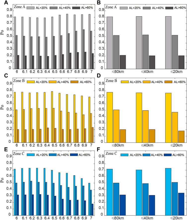
FIGURE 2. Seismo-ionospheric anomalies occurrence probabilities of AL>20%, 40%, and 60% with different magnitudes (A, C, E) and depths (B, D, F), respectively (15-day sliding window). (A, C) are the results in Zone A. (C, D) are the results in Zone B. (E, F) are the results in Zone C.

TABLE 1

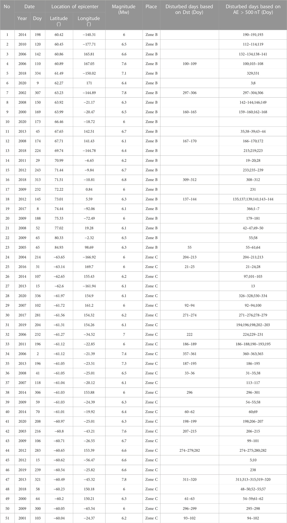
TABLE 1. The difference of disturbed days based on Dst and AE before 51 Earthquakes at high latitudes.

According to Figure 2 (right), one can find that the values of $P_o$ decrease in Zone A and C, and increase in Zone B slightly, with depths increasing. The maximum difference of $P_o$ between different depths in Zone A, B and C was 0.0075, 0.0372 and 0.0291, respectively. Therefore, it reveals that for shallow earthquakes (≤60 km), the influence of depths on $P_o$ could be ignored. For the case of AL>20% or AL>40%, the results of Zone A are the largest, followed by those of Zone B. For the case of AL>60%, the results of Zone C are the largest, while the rest two zones have no significant difference. Therefore, selecting different AL has an obvious impact on $P_o$ in different zones with different magnitudes and depths. Considering that all the earthquakes in this study are shallow earthquakes, the impact of different depths will not be further investigated in the following sections.

To study the effects of different lengths of the sliding windows on $P_o$, Figure 3 shows the differences between the results of different sliding windows, indicating the effect of sliding window length on latitudinal zones, that is, the most affected zones are Zone C, B and A in decreasing order. For the earthquakes in the southern mid- and high-latitude region (Zone C), compared with the results of 15-day sliding window: 1) the results of 10-day or 27-day sliding window are systematically increased, and the differences are larger using 27-day sliding window; 2) For the cases of AL>20% or AL>40%, most of the relative changes are less than 20%, while the maximum difference and relative change can reach 0.16% and 80%, respectively with AL>60%. Moreover, the differences increase with the increase of the magnitude selecting AL>60%.

FIGURE 3

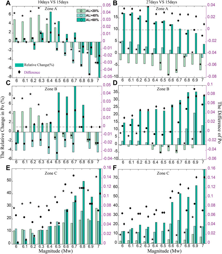
FIGURE 3. The differences and relative changes of seismo-ionospheric anomalies occurrence probabilities between the results of different sliding windows. (A, C, E) show the difference between the results of 10-day and 15-day sliding windows in Zone A, Zone B and Zone C, respectively. (B, D, F) show the difference between the results of 27-day and 15-day sliding windows in Zone A, Zone B and Zone C, respectively.

For the earthquakes in the northern mid- and high-latitude region (Zone B), compared with the results of 15-day sliding window: 1) most differences are random, and are also greater using 27-day sliding window; 2) For the cases of AL>20% or AL>40%, most relative changes are between −6% and 10%. For the cases of AL>60%, the 27-day results increase systematically, and the maximum difference and relative change can reach 0.092% and 35.71%, respectively.

For the earthquakes in the low-latitude and equatorial region (Zone A), compared with the results of 15-day sliding window: 1) the results vary systematically using the 27-day sliding window; 2) For the cases of AL> 20% or AL>40%, most relative changes are between −8% and 8%. For the cases of AL>60%, the 27-day results increase systematically and the differences decrease with the magnitude increasing, with the maximum difference and relative change reaching 0.039% and 19.59%, respectively.

When AL > 20% or AL > 40% is selected to extract seismo-ionospheric anomalies, most of the relative changes of different sliding window are under 20%. In this study, GIM produced by the Jet Propulsion Laboratory (JPL) is used, and the error of VTEC estimation during the creating process of global maps by JPL is about 10%–17% (Zakharenkova et al., 2008). Therefore, for the case of AL > 20% or AL > 40%, different lengths of sliding windows have a statistically insignificant influence on $P_o$. When AL>60% is selected, different lengths of sliding windows have non-negligible impacts on $P_o$ in the mid- and high-latitude region, particularly in the southern Hemisphere where there are obvious systematic deviations between the results of different sliding windows. The reasons for the observed systematic deviations may include: 1) the real effects of different lengths of sliding windows; 2) the number of GNSS stations in the southern Hemisphere is smaller than those in the northern Hemisphere, resulting in larger error of VTEC in the southern Hemisphere; 3) the number of earthquakes in Zone C is the smallest. 4) external magnetic fields contamination is still probably not excluded in this study for some earthquakes in Zone B and Zone C (Table 1). However, it can be noted that in Zone A, there are also obvious systematic deviations between the results of 15-day and 27-day sliding windows, indicating the influence of different sliding window lengths cannot be ignored.

Figure 4 shows the Index Number in percentage of the seismo-ionospheric anomalies within 1–10 days before the earthquakes. The Index Number is calculated as the ratio of the cumulative number of seismo-ionospheric anomalies in a single day and the total number of seismo-ionospheric anomalies (Shah et al., 2020). The Index Number enhances within 5 days before the earthquakes in all the three zones, especially in Zone A and B. Figures 5, 6 show the differences and relative changes between the results of different sliding windows. It can be seen that the differences between the results of different sliding windows are random, and are larger between the results of 15-day and 27-day sliding windows. The differences are smallest in Zone A, followed by Zone B. The differences raise with AL increasing. For the case of AL>20% or AL>40%, compared with the results of 15-day sliding window, the most of relative changes are between −20% and 25%. For the case of AL > 60%, the differences are more significant, as the relative changes can exceed 50% in all the three zones. So when AL>60% is selected, the impacts of different sliding windows on the Index Number can not be neglected.

FIGURE 4

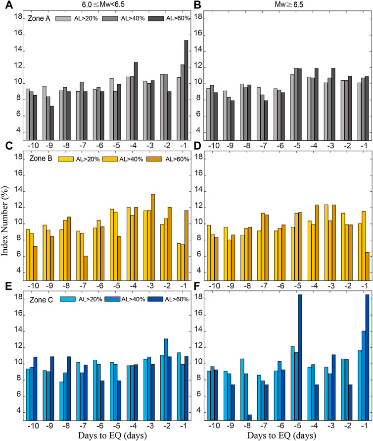
FIGURE 4. The Index Numbers of the seismo-ionospheric anomalies within 1-10 days before the global earthquakes during 2000-2020 (15-day sliding window). (A, C, E) are the results of 6.0≤Mw<6.5 in Zone A, Zone B and Zone C, respectively. (B, D, F) are the results of Mw≥6.5 in Zone A, Zone B and Zone C, respectively.

FIGURE 5

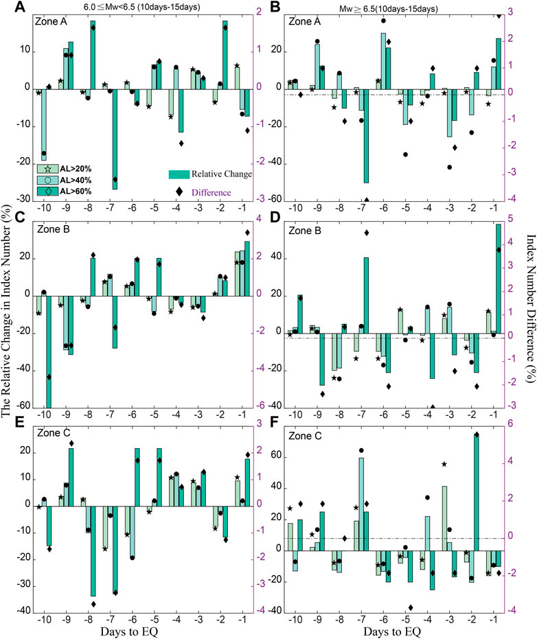
FIGURE 5. The differences and relative changes of the Index Numbers of the seismo-ionospheric anomalies between the results of 10-day and 15-day sliding windows. (A, C, E) represent the results of 6.0≤Mw<6.5 in Zone A, Zone B and Zone C, respectively. (B, D, F) represent the results of Mw≥6.5 in Zone A, Zone B and Zone C, respectively.

FIGURE 6

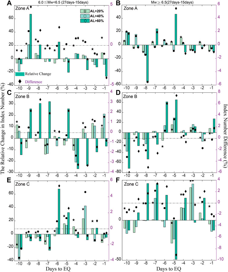
FIGURE 6. The differences and relative changes of the Index Numbers of the seismo-ionospheric anomalies between the results of 27-day and 15-day sliding windows. (A, C, E) represent the results of 6.0≤Mw<6.5 in Zone A, Zone B and Zone C, respectively. (B, D, F) represent the results of Mw≥6.5 in Zone A, Zone B and Zone C, respectively.

3.2 Seismo-ionospheric anomalies occurrence rates

According to Eq. 2, seismo-ionospheric anomalies occurrence rates $P_E$ are obtained for all the three zones. Figure 7 shows $P_E$ with AL>20%, AL>40% and AL>60% within 1–10 days before different magnitude earthquakes. We found that the larger magnitude of earthquakes and the closer prior to the earthquake occurrence, the larger values of $P_E$. For instance, the value of $P_E$ increases from 26.82% for Mw≥6.0 earthquakes to 31.29% for Mw≥7.0 earthquakes 1 day before the earthquakes. It can be seen that the correlation is not obvious between the values of $P_E$ in Zone C and the magnitude with AL>60%. It needs to be taken into account with the time (for example, 1–5 days prior to the earthquakes) and the latitude of the epicenter (for example, in the low-latitude and equatorial region) that the values of $P_E$ increase with the magnitude increasing. In addition, as mentioned in the previous section, the number of earthquakes is smaller and the errors of VTEC are larger in Zone C, so the results in Zone C could be biased to some extent. Besides, the effects of external magnetic fields contamination for some earthquakes in Zone B and Zone C may not be excluded, which would also bias the results.

FIGURE 7

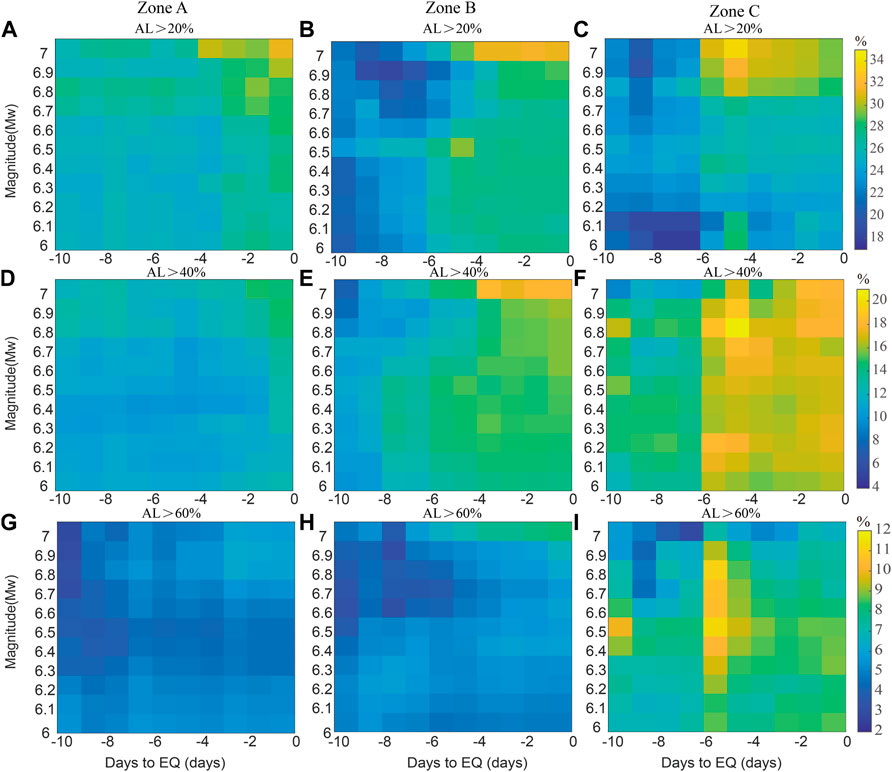
FIGURE 7. Seismo-ionospheric anomalies occurrence rates of AL>20%, 40%, and 60% within 1-10 days before earthquakes of Zone A (A, D, G), Zone B (B, E, H), and Zone C (C, F, I), respectively (15-day sliding window).

Figures 8, 9 represent the $P_E$ differences of the results using different sliding windows. For Zone A, different sliding window lengths have little influence. For Zone B, compared with the results of the 15-day sliding window, the values of $P_E$ significantly increase for Mw≥6.7 earthquakes using 27-day sliding window. For Zone C, the differences of the results of different sliding windows are larger than those in the other zones without systematic pattern. Therefore, it indicates that the impacts of sliding window lengths are related to the latitude of the epicenter. Different sliding windows should be selected to investigate the earthquakes in different zones. For Zone A, 10-day, 15-day and 27-day sliding windows may be selected arbitrarily. For Zone B, 27-day sliding window may be a better choice. But the selection of the optimal sliding window for Zone C still needs further research in the future.

FIGURE 8

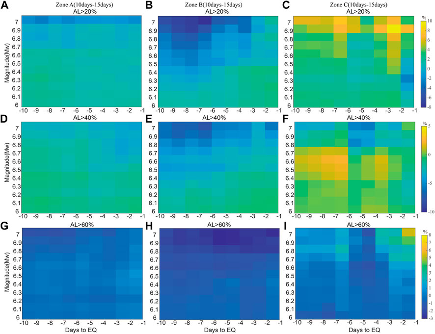
FIGURE 8. The differences of seismo-ionospheric anomalies occurrence rates between the results of 10-day and 15-day sliding windows. (A, D, G) represent the results in Zone A. (B, E, H) represent the results in Zone B. (C, F, I) represent the results in Zone C.

FIGURE 9

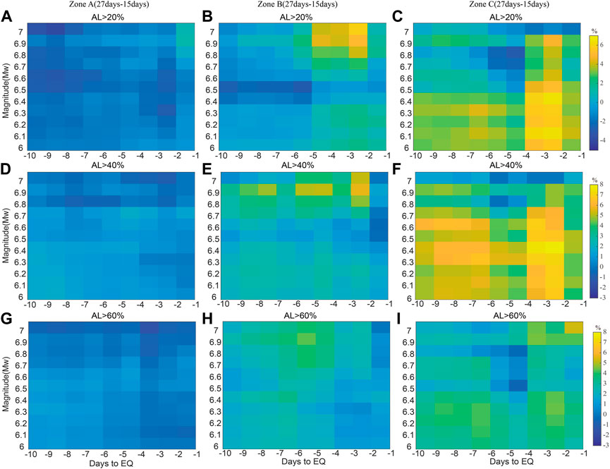
FIGURE 9. The differences of seismo-ionospheric anomalies occurrence rates between the results of 27-day and 15-day sliding windows. (A, D, G) represent the results in Zone A. (B, E, H) represent the results in Zone B. (C, F, I) represent the results in Zone C.

To compare the difference between the seimo-ionospheric anomalies a few days before the earthquakes and the day-to-day ionospheric variation, the ionospheric anomalies occurrence rates during background days $P_N$, as shown in Eq. 3, derived from Le et al. (2011), are also calculated. For each earthquake, 61–300 days before this earthquake are selected as the background days, and disturbed days $\Delta W$ by geomagnetic storms and by the Mw≥6.0 earthquakes at the adjacent places are also excluded.

$P_N=\frac{{\displaystyle \sum _{n=1}^K}{N}_{AL}^n}{K\times 240-\Delta W}(3)$

In this equation, $K$ is the number of earthquakes in each group (for example, Mw ≥ 6.5 in Zone A with AL>20%); $N_{AL}^n$ is the number of seismo-ionospheric days with different AL (for example, AL>20%) during the 61–300 days before the $n$ th earthquake; $\Delta W$ is the number of disturbed days.

Figure 10A shows the values of $P_N$ for different magnitude earthquakes. The results are smaller than those of $P_E$, and seem to decrease very slightly with the magnitude increasing. The effects of different latitudinal locations and AL on the values of $P_N$ is insignificant. Figures 10B, C) presents the differences of $P_N$ derived from different sliding window lengths are obviously systematic, and are related to AL. For example, when AL > 20% is assumed, all the results of 27-day sliding window are reduced compared with those of 15-day sliding window. Therefore, different sliding window lengths have a systematic effect on the values of $P_N$.

FIGURE 10

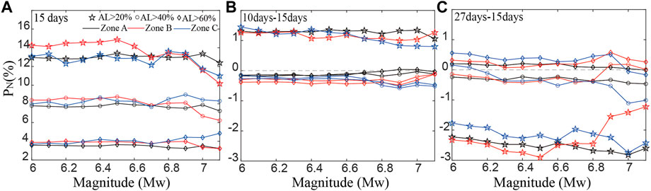
FIGURE 10. (A) Ionospheric anomalies occurrence rates of A >20%, 40%, and 6% during background days; (B) The differences of ionospheric anomalies occurrence rates between the results of 10-day and 15-day sliding windows; (C) The differences of ionospheric anomalies occurrence rates between the results of 27-day and 15-day sliding windows.

Figure 11 shows the ratio of $P_E$ and $P_N$ with different magnitude using 15-day sliding window. The results show that most of the values of $P_E/P_N$ are larger than 1, indicating large differences of the occurrence rates between the days prior to earthquakes and the background days.

FIGURE 11

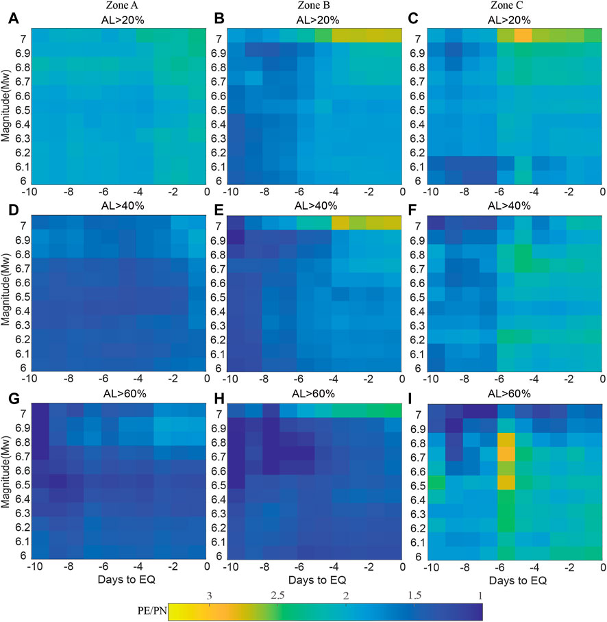
FIGURE 11. The ratio of the seimo-ionospheric anomalies occurrence rates within 1-10 days before the earthquakes to the ionospheric anomalies occurrence rates during background days (15-day sliding window). (A, D, G) represent the results in Zone A. (B, E, H) represent the results in Zone B. (C, F, I) represent the results in Zone C.

4 Conclusion

Both the latitude of the epicenter and the magnitude can affect the characteristics of seismo-ionospheric anomalies before shallow earthquakes. In terms of seismo-ionospheric anomalies occurrence probabilities $P_o$, ionospheric enhancement in the low-latitude and equatorial region is more significant (Zone A), and their $P_o$ are larger with the magnitude increasing, especially for Mw≥6.6 earthquakes; in the mid- and high-latitude region (Zone B and C), a slight negative correlation is presented between the values of $P_o$ and the magnitude. In terms of seismo-ionospheric anomalies occurrence rates $P_E$, the values of $P_E$ increase with the magnitude increasing in all the three zones, but the correlation between the values of $P_E$ and the magnitude is faint in Zone C. Because of the small number of earthquakes and the low accuracy of VTEC in Zone C, the reliability of the results still needs to be further studied and confirmed.

Both the number of days before earthquakes and the AL can affect the characteristics of seismo-ionospheric anomalies before shallow earthquakes. The number of seismo-ionospheric anomalies within 1–5 days before the earthquakes increases significantly in all the three zones, and the positive correlation between the values of $P_E$ and the magnitude is more strong within 1–5 days before the earthquakes. For the case of AL>20% and AL>40%, the values of $P_o$ in the low-latitude and equatorial region are higher than those in the mid- and high-latitude region; For the case of AL>60%, the values of $P_o$ in the southern mid- and high-latitude region are higher than those in the other zones before 6.0≤Mw < 6.7 earthquakes. Therefore, when seismo-ionospheric anomalies in different regions are analyzed, the choice of AL may affect the outcome significantly.

For the mid- and high-latitude region, the effects of different lengths of sliding windows on seismo-ionospheric anomalies can not be ignored. For the case of AL>60%, different sliding windows have a significant impact on the values of $P_o$ and $P_E$_, and there are systematic deviations between the values of $P_o$ using different sliding windows in the southern mid- and high-latitude region. However, the selection of the optimal sliding window needs to be further studied, especially for the Zone C.

Moreover, there are large differences between the seismo-ionospheric anomalies occurrence rates $P_E$ 1–10 days prior to the earthquakes and ionospheric anomalies occurrence rates $P_N$ during the background days, indicating that the seismo-ionospheric anomalies within just a few days before the earthquakes are probably related with the forthcoming earthquakes. The 1522 earthquakes in this study are divided into multiple groups, resulting in the small number of earthquakes in some groups, and the accuracy of VTEC in different regions is uneven, which may bias the results in this study. Although the earthquakes occurring at the similar location but with the short interval (<10 days) from the previous ones are excluded, some earthquakes occurring close to their boundaries in two confining zones may also have some confounded effects on the results. Besides, whether a pixel of $2.5^{\circ }\times 5^{\circ }$ is appropriate for the earthquakes larger than Mw6.0 needs to be further studied.

Data availability statement

The raw data supporting the conclusion of this article will be made available by the authors, without undue reservation.

Author contributions

MY and ZX contributed to conception of the study. Data were collected by HL, DH, and YR. MY, ZX, and YY performed the experimental analysis. MY wrote the first draft of the manuscript. ZX revised the manuscript. All authors read and approved the final manuscript.

Funding

This work was supported by Beijing Natural Science Foundation Grant Numbers 8224094.

Acknowledgments

We are grateful to the World Data Center for Geomagnetism, Kyoto providing Dst index, the Global CMT Project providing parameters of earthquakes, and IGS providing GIM.

Conflict of interest

The authors declare that the research was conducted in the absence of any commercial or financial relationships that could be construed as a potential conflict of interest.

Publisher’s note

All claims expressed in this article are solely those of the authors and do not necessarily represent those of their affiliated organizations, or those of the publisher, the editors and the reviewers. Any product that may be evaluated in this article, or claim that may be made by its manufacturer, is not guaranteed or endorsed by the publisher.

References

Dautermann, T., Calais, E., Haase, J., and Garrison, J. (2007). Investigation of ionospheric electron content variations before earthquakes in southern California, 2003-2004. J. Geophys. Res. 112, 1074–1086. doi:10.1029/2006JB004447

CrossRef Full Text | Google Scholar

Davidenko, D. V., and Pulinets, S. A. (2019). Deterministic variability of the ionosphere on the eve of strong (M≥6) earthquakes in the regions of Greece and Italy according to long-term measurements data. Geomagn. Aeron. 59 (4), 493–508. doi:10.1134/S001679321904008X

CrossRef Full Text | Google Scholar

De Santis, A., Marchetti, D., Pavón-Carrasco, F. J., Cianchini, G., Perrone, L., Abbattista, C., et al. (2019). Precursory worldwide signatures of earthquake occurrences on Swarm satellite data. Sci. Rep. 9, 20287. doi:10.1038/s41598-019-56599-1

PubMed Abstract | CrossRef Full Text | Google Scholar

Dobrovolsky, I. P., Zubkov, S. I., and Miachkin, V. I. (1979). Estimation of the size of earthquake preparation zones. Pure Appl. Geophys. 117 (5), 1025–1044. doi:10.1007/BF00876083

CrossRef Full Text | Google Scholar

Freund, F. (2011). Pre-earthquake signals: Underlying physical processes. J. Asian Earth Sci. 41 (4-5), 383–400. doi:10.1016/j.jseaes.2010.03.009

CrossRef Full Text | Google Scholar

Fujiwara, H., Kamogawa, M., Ikeda, M., Liu, J. Y., Sakata, H., Chen, Y. I., et al. (2004). Atmospheric anomalies observed during earthquake occurrences. Geophys. Res. Lett. 31, L17110. doi:10.1029/2004GL019865

CrossRef Full Text | Google Scholar

Guo, J., Li, W., Yu, H., Liu, Z., Zhao, C., and Kong, Q. (2015). Impending ionospheric anomaly preceding the Iquique Mw8.2 earthquake in Chile on 2014 April 1. Geophys. J. Int. 203 (3), 1461–1470. doi:10.1093/gji/ggv376

CrossRef Full Text | Google Scholar

Hernández-Pajares, M., Juan, J., Sanz, J., Orus, R., Garcia-Rigo, A., Feltens, J., et al. (2009). The IGS VTEC maps: A reliable source of ionospheric information since 1998. J. Geod. 83 (3-4), 263–275. doi:10.1007/s00190-008-0266-1

CrossRef Full Text | Google Scholar

Ho, Y. Y., Jhuang, H. K., Su, Y. C., and Liu, J. Y. (2013). Seismo-ionospheric anomalies in total electron content of the GIM and electron density of DEMETER before the 27 February 2010 M8.8 Chile earthquake. Adv. Space Res. 51 (12), 2309–2315. doi:10.1016/j.asr.2013.02.006

CrossRef Full Text | Google Scholar

Jiang, W., Ma, Y., Zhou, X., Li, Z., An, X., and Wang, K. (2017). Analysis of ionospheric vertical total electron content before the 1 April 2014 Mw 8.2 Chile earthquake. J. Seismol. 21 (6), 1599–1612. doi:10.1007/s10950-017-9684-y

CrossRef Full Text | Google Scholar

Ke, F., Wang, Y., Wang, X., Qian, H., and Shi, C. (2016). Statistical analysis of seismo-ionospheric anomalies related to Ms>5.0 earthquakes in China by GPS TEC. J. Seismol. 20 (1), 137–149. doi:10.1007/s10950-015-9516-x

CrossRef Full Text | Google Scholar

Klimenko, M. V., Klimenko, V. V., Zakharenkova, I. E., and Pulinets, S. A. (2012). Variations of equatorial electrojet as possible seismo-ionospheric precursor at the occurrence of TEC anomalies before strong earthquake. Adv. Space Res. 49 (3), 509–517. doi:10.1016/j.asr.2011.10.017

CrossRef Full Text | Google Scholar

Kon, S., Nishihashi, M., and Hattori, K. (2011). Ionospheric anomalies possibly associated with M ≥ 6.0 earthquakes in the Japan area during 1998–2010: Case studies and statistical study. J. Asian Earth Sci. 41 (4), 410–420. doi:10.1016/j.jseaes.2010.10.005

CrossRef Full Text | Google Scholar

Le, H., Liu, J. Y., and Liu, L. (2011). A statistical analysis of ionospheric anomalies before 736 M6.0+ earthquakes during 2002-2010. J. Geophys. Res. 116 (A2), A02303. doi:10.1029/2010JA015781

CrossRef Full Text | Google Scholar

Liperovsky, V. A., Pokhotelov, O. A., Meister, C. V., and Liperovskaya, E. V. (2008). Physical models of coupling in the lithosphere-atmosphere-ionosphere system before earthquakes. Geomagn. Aeron. 48, 795–806. doi:10.1134/S0016793208060133

CrossRef Full Text | Google Scholar

Liu, J. Y., Chen, C. H., Chen, Y. I., Yang, W. H., Oyama, K. I., and Kuo, K. W. (2010). A statistical study of ionospheric earthquake precursors monitored by using equatorial ionization anomaly of GPS TEC in Taiwan during 2001–2007. J. Asian Earth Sci. 39 (1), 76–80. doi:10.1016/j.jseaes.2010.02.012

CrossRef Full Text | Google Scholar

Liu, J. Y., Chen, Y. I., Chuo, Y. J., and Tsai, H. F. (2001). Variations of ionospheric total electron content during the Chi-Chi earthquake. Geophys. Res. Lett. 28 (7), 1383–1386. doi:10.1029/2000GL012511

CrossRef Full Text | Google Scholar

Liu, J. Y., Chuo, Y. J., Shan, S. J., Tsai, Y. B., Chen, Y. I., Pulinets, S. A., et al. (2004). Pre-earthquake ionospheric anomalies registered by continuous GPS TEC measurements. Ann. Geophys. 22 (5), 1585–1593. doi:10.5194/angeo-22-1585-2004

CrossRef Full Text | Google Scholar

Liu, W., and Xu, L. (2017). Statistical analysis of ionospheric TEC anomalies before global Mw≥7.0 earthquakes using data of CODE GIM. J. Seismol. 21 (4), 759–775. doi:10.1007/s10950-016-9634-0

CrossRef Full Text | Google Scholar

Ma, X., Lin, Z., and Chen, H. (2014). Analysis on ionospheric perturbation of TEC and NmF2 based on GPS and COSMIC data before and after the Wenchuan earthquake. Chin. J. Geophys 57 (8), 2415–2422. doi:10.6038/cjg20140803

CrossRef Full Text | Google Scholar

Masci, F. (2012). The study of ionospheric anomalies in Japan area during 1998–2010 by Kon et al.: An inaccurate claim of earthquake-related signatures? J. Asian Earth Sci. 57, 1–5. doi:10.1016/j.jseaes.2012.06.009

CrossRef Full Text | Google Scholar

Masci, F., and Thomas, J. (2014). Comment on “Temporal and spatial precursors in ionospheric total electron content of the 16 October 1999 M_w  7.1 Hector Mine earthquake” by Su et al. (2013). J. Geophys. Res. 119, 6994–6997. doi:10.1002/2014JA019896

CrossRef Full Text | Google Scholar

Michael, A. J. (2011). Random variability explains apparent global clustering of large earthquakes. Geophys. Res. Lett. 38, L21301. doi:10.1029/2011GL049443

CrossRef Full Text | Google Scholar

Namgaladze, A. A., Klimenko, M. V., Klimenko, V. V., and Zakharenkova, I. E. (2009). Physical mechanism and mathematical modeling of earthquake ionospheric precursors registered in total electron content. Geomagn. Aeron. 49 (2), 252–262. doi:10.1134/S0016793209020169

CrossRef Full Text | Google Scholar

Nishihashi, M., Hattori, K., Jhuang, H. K., and Liu, J. Y. (2009). Possible spatial extent of ionospheric GPS-TEC and NmF2 anomalies related to the 1999 Chi-Chi and Chia-Yi earthquakes in Taiwan. Terr. Atmos. Ocean. Sci. 20, 779–789. (T). doi:10.3319/tao.2009.01.22.01(t)

CrossRef Full Text | Google Scholar

Ovalle, E., Villalobos, C., Bravo, M., and Foppiano, A. (2013). Maximum electron concentration and total electron content of the ionosphere over Concepción, Chile, prior to the 27 February 2010 earthquake. Adv. Space Res. 52, 1274–1288. doi:10.1016/j.asr.2013.07.005

CrossRef Full Text | Google Scholar

Parrot, M., and Li, M. (2018). “Statistical analysis of the ionospheric density recorded by DEMETER during seismic activity,” In pre-earthquake processes: a multidisciplinary approach to earthquake prediction studies (geophysical monograph 234). Editors D. Ouzounov, S. Pulinets, K. Hattori, and P. Taylor (Washington, DC: American Geophysical Union John Wiley and Sons, Inc.).

Google Scholar

Pulinets, S. A., and Boyarchuk, K. (2004). Ionospheric precursors of earthquakes. Berlin: Springer Press.

Google Scholar

Pulinets, S. A., and Davidenko, D. V. (2018). The nocturnal positive ionospheric anomaly of electron density as a short-term earthquake precursor and the possible physical mechanism of its formation. Geomagn. Aeron. 58, 559–570. doi:10.1134/s0016793218040126

CrossRef Full Text | Google Scholar

Pulinets, S. A., Krankowski, A., Hernandez-Pajares, M., Marra, S., Budnikov, P., Zakharenkova, I., et al. (2021). Ionosphere sounding for pre-seismic anomalies identification (INSPIRE): Results of the Project and perspectives for the short-term earthquake forecast. Front. Earth Sci. 9, 610193. doi:10.3389/feart.2021.610193

CrossRef Full Text | Google Scholar

Pulinets, S. (2012). Low-latitude atmosphere-ionosphere effects initiated by strong earthquakes preparation process. Int. J. Geophys 2012, 1–14. doi:10.1155/2012/131842

CrossRef Full Text | Google Scholar

Pulinets, S., and Ouzounov, D. (2011). Lithosphere-Atmosphere-Ionosphere Coupling (LAIC) model-An unified concept for earthquake precursors validation. J. Asian Earth Sci. 41 (4), 371–382. doi:10.1016/j.jseaes.2010.03.005

CrossRef Full Text | Google Scholar

Rishbeth, H. (2006). Ionoquakes: Earthquake precursors in the ionosphere? Eos. Trans. Am. Geophys. Union 87, 316. doi:10.1029/2006EO320008

CrossRef Full Text | Google Scholar

Shah, M., Ahmed, A., Ehsan, M., Khan, M., Tariq, M. A., Calabia, A., et al. (2020). Total electron content anomalies associated with earthquakes occurred during 1998-2019. Acta Astronaut. 175, 268–276. doi:10.1016/j.actaastro.2020.06.005

CrossRef Full Text | Google Scholar

Shah, M., and Jin, S. (2015). Statistical characteristics of seismo-ionospheric GPS TEC disturbances prior to global Mw≥5.0 earthquakes (1998–2014). J. Geodyn. 92, 42–49. doi:10.1016/j.jog.2015.10.002

CrossRef Full Text | Google Scholar

Su, Y. C., Liu, J. Y., Chen, S. P., Tsai, H. F., and Chen, M. Q. (2013). Temporal and spatial precursors in ionospheric total electron content of the 16 october 1999M_w7.1 hector mine earthquake: Ionoquack OFM7.1 hector mine earthquake. J. Geophys. Res. 118 (10), 6511–6517. doi:10.1002/jgra.50586

CrossRef Full Text | Google Scholar

Sun, Y., Liu, J., Lin, C., Tsai, H. F., Chang, L. C., Chen, C. Y., et al. (2016). Ionospheric f2 region perturbed by the 25 april 2015 Nepal earthquake: Ionosphere perturbed by Nepal earthquake. J. Geophys. Res. 121, 5778–5784. doi:10.1002/2015JA022280

CrossRef Full Text | Google Scholar

Tang, J., Yao, Y., and Zhang, L. (2015). Temporal and spatial ionospheric variations of 20 April 2013 earthquake in Yaan, China. IEEE Geosci. Remote Sens. Lett. 12, 2242–2246. doi:10.1109/LGRS.2015.2463081

CrossRef Full Text | Google Scholar

Xu, T., Chen, Z., Li, C., Wu, J., Hu, Y., and Wu, Z. (2011). GPS total electron content and surface latent heat flux variations before the 11 March 2011 M9.0 Sendai earthquake. Adv. Space Res. 48 (8), 1311–1317. doi:10.1016/j.asr.2011.06.024

CrossRef Full Text | Google Scholar

Yao, Y., Chen, P., Wu, H., Zhang, S., and Peng, W. (2012). Analysis of ionospheric anomalies before the 2011 Mw 9.0 Japan earthquake. Chin. Sci. Bull. 57, 500–510. doi:10.1007/s11434-011-4851-y

CrossRef Full Text | Google Scholar

Zakharenkova, I. E., Shagimuratov, I. I., Tepenitzina, N. Y., and Krankowski, A. (2008). Anomalous modification of the ionospheric total electron content prior to the 26 September 2005 Peru earthquake. J. Atmos. Sol-terr. Phy. 70 (15), 1919–1928. doi:10.1016/j.jastp.2008.06.003

CrossRef Full Text | Google Scholar

Zhang, X., Shen, X., Zhao, S., Yao, L., Ouyang, X., and Qian, J. (2014). The characteristics of quasistatic electric field perturbations observed by DEMETER satellite before large earthquakes. J. Asian Earth Sci. 79 (2), 42–52. doi:10.1016/j.jseaes.2013.08.026

CrossRef Full Text | Google Scholar

Zhou, Y., Wu, Y., Qiao, X., and Zhang, X. (2009). Ionospheric anomalies detected by ground-based GPS before the Mw7.9 Wenchuan earthquake of May 12, 2008, China. J. Atmos. Sol-terr. Phy. 71, 959–966. doi:10.1016/j.jastp.2009.03.024

CrossRef Full Text | Google Scholar

Zhu, F., Zhou, Y., Lin, J., and Su, F. (2014). A statistical study on the temporal distribution of ionospheric TEC anomalies prior to M7.0+ earthquakes during 2003-2012. Astrophys. Space Sci. 350, 449–457. doi:10.1007/s10509-014-1777-2

CrossRef Full Text | Google Scholar

Zolotov, O. V., Knyazeva, M. A., and Romanovskaya, Y. V. (2019). Computer analysis of total electron content in the Earth’s ionosphere in problems of searching for and detection of earthquake precursors: Current problems and challenges. Russ. J. Phys. Chem. B 13 (4), 681–684. doi:10.1134/S1990793119040146

CrossRef Full Text | Google Scholar

Zolotov, O. V., Namgaladze, A. A., Zakharenkova, I. E., Martynenko, O. V., and Shagimuratov, I. I. (2012). Physical interpretation and mathematical simulation of ionospheric precursors of earthquakes at midlatitudes. Geomagn. Aeron. 52 (3), 390–397. doi:10.1134/S0016793212030152

CrossRef Full Text | Google Scholar