 Liming Zhou1
 Shiqi Dong
 Pan Zhang
- 1Key Laboratory of Geotechnical Mechanics and Engineering of the Ministry of Water Resources, Changjiang River Scientific Research Institute, Wuhan, China
- 2College of Geo-Exploration Science and Technology, Jilin University, Changchun, China
- 3School of Resources and Geosciences, China University of Mining and Technology, Xuzhou, China
Cycle skipping problem caused by the absent of low frequencies and inaccurate initial model makes full waveform inversion (FWI) deviate from the true model. A novel method is proposed to mitigate cycle skipping phenomenon by dynamic data matching which improves the matching of synthetic and observed events to regulate the updating of initial model in a correct direction. 1-dimentional (1-D) Gaussian convolutional kernels with different lengths are used to extract features of each time sample in each trace which represents the integrated properties of wavefield at different time ranges centered on each time sample. According to the minimum Euclidean distance of the features, the optimally matched pairs of time samples in the observed and synthetic trace can be found. A constraint evaluates the reliability of dynamic matching by attenuating the amplitude of synthetic data according to the values of traveltime differences between each pairs of optimally matched time samples is proposed to improve the accuracy of data matching. In addition, Gaussian kernels have the capability to extract features of time samples contaminated by strong noises accurately to improve the robustness of the propose method further. The selection scheme of optimal parameters is discussed and concluded to ensure the convergence of the proposed method. Numerical tests on Marmousi model verify the feasibility of the propose method. The proposed method provides a new approach to tackle the convergence problem of FWI when using the field seismic data.
1 Introduction
Full waveform inversion (FWI) suffers from the cycle skipping problem, which leads FWI to converge to the local minima (Virieux and Operto, 2009). Sufficiently low frequencies in observed data and a suitable initial model are important for FWI to overcome cycle skipping (Bunks et al., 1995). However, it is difficult to provide a good initial model for FWI without sufficient prior information, with low frequency components usually absent from seismic field data. Therefore, many researchers have devoted much to solving the cycle skipping phenomenon from different perspectives. There are three main approaches to addressing this issue.
First, artificial low frequencies, which are similar to the low-frequency components of the intact observed data that conveys long wavelength information of subsurface media, can be introduced into FWI. Chi et al. (2014) utilized the differences between the envelopes of both observed and calculated data as a misfit function to provide the long-wavelength components of the subsurface velocity for standard FWI. Liu et al. (2018) fitted the intensity of the observed and synthetic data and found that sufficiently low frequencies in intensity data can help FWI avoid cycle skipping. Sun and Demanet (2018) extrapolated low frequencies from the band-limited signals by a one-dimensional (1-D) convolutional neural network (CNN), which learns non-linear mapping between training sets and labels. Yang et al. (2022) developed a deep learning-based approach for low frequency reconstruction in which high frequencies are transformed into low frequencies by training an end-to-end three-dimensional (3D) CNN.
Second, waveform-matching techniques can be used to avoid cycle skipping. Wang et al. (2016) used dynamic time warping (DTW), which can detect the travel-time difference between synthetic and observed data to help FWI avoid cycle skipping. Dong S. et al., 2020 proposed a local travel time correction approach to decrease travel-time differences between waveforms to improve waveform matching. Chen et al. (2022) proposed a penalized differential DTW misfit function to further identify the travel-time difference between observed and synthetic data.
Third, data (or model, acquisition) extension and measurement of the differences between the observed and synthetic data in the transformation domain improves the convexity of misfit functions. Zhu and Fomel (2016) proposed adaptive matching filtering-based FWI which measures time-varying phase differences between the observed and predicted data. Huang et al. (2017) proposed the regularized formulation of source-receiver extended inversion to recover reasonably good velocity models from synthetic transmission and reflection data. Barnier et al. (2018) introduced model extension to FWI by adding a correcting term to ensure phase matching between the observed and predicted data. Huang et al. (2021) used the time-warping function as the extension in the data space to solve the velocity model and time-warping extension in a single optimization problem by the alternate direction method. Some other solutions, such as gradient sampling (Yang et al., 2020), wavefield reconstruction (Rizzuti et al., 2021), Bayesian non-linear inversion (Guo et al., 2020), wide-angle seismic acquisition (Guo et al., 2022), and global optimization (Mojica and Kukreja, 2019), can also mitigate cycle skipping.
In addition, field seismic data are usually contaminated by noise (both random and coherent), which also causes FWI to deviate from the correct direction of convergence. Conventional denoising methods (e.g., f-x deconvolution, EMD, SVD, and wavelet transform) are usually based on theoretical model assumptions and rely on a priori information, which has difficulty handling complex noises and low computational efficiency (Han and Van, 2015; Liu and Zheng, 2022). Data-driven-based denoising methods can establish a strong non-linear mapping between noise-contained and pure data, which is currently a hot research topic in seismic denoising. Dong et al. (2019) and Dong X. et al. (2020) used DnCNNs to predict noise in field desert data acquired from the Tarim region in China. Zhang et al. (2021) used a UNet structure to suppress surface-related multiple labels with synthetic primary labels. Dong et al. (2022a) proposed a multiscale spatial attention network to suppress strong noises and recover weak reflections. Dong et al. (2022b) proposed a novel strategy to generate sufficient real noise by a generative adversarial network (GAN), which compensates for the lack of real noise data.
There is a weak similarity between observed and the synthetic data, especially when the initial model is inaccurate, which indicates different travel times between the observed and synthetic traces existing in different pairs of events. Inspired by the ideas from the features extraction of CNN and dynamic data matching of DTW, we propose a novel approach to achieve global-searching-based dynamic data matching by the similarity of features of each time sample in the observed and synthetic traces. We use 1-D Gaussian convolutional kernels to extract features of each time sample in a single seismic trace, with the features representing the integrated properties of wavefield (amplitude, phase and travel time, etc.). In order to highlight the representation of convolution-based features for each time sample, we use Gaussian kernels with different lengths to extract the features at different time ranges centered on each time sample; this is the same way in which CNN extracts features of different scales from images through convolutional kernels of different receptive fields. According to the minimum Euclidean distance of the features, only the time sample in the observed data that optimally matches the time sample in the synthetic data of the same trace number can be found. Synthetic time samples are time-shifted to align the optimally matched observed time samples to accomplish dynamic data matching. However, not every observed event can be optimally matched to a synthetic event. Thus, it is necessary to introduce a constraint to evaluate the reliability of each dynamic matching pair. We propose that the amplitude of the synthetic time sample after dynamic matching attenuate as the absolute value of shifted time increases, which means that a pair of optimally matched time samples with large time differences will be more likely regarded as mismatched, and we attenuate these data artificially to mitigate their interference to the gradient. After the steps introduced previously, intermediate synthetic data can be generated by dynamic data matching, which regulates the model to update in correct directions. Meanwhile, although denoising methods improve the signal to noise ratio (SNR) of the observed data, effective seismic signals will also experience some damage. Gaussian kernels have a strong ability to extract accurate features from noised-contained seismic traces without an extra denoising process, thus ensuring that the extracted features do not experience interference from other objective factors. Furthermore, the proposed novel method can be combined with encoded multi-source to accelerate the iterations of FWI. Numerical tests have demonstrated the feasibility of our method.
2 Methods
2.1 Feature extraction
Features from the input data were extracted by the convolutional kernels of CNN. Based on this function of convolution, we used 1-D Gaussian kernels to extract features of the synthetic and observed data trace by trace. We regarded the convolution value as the feature of each time sample when the kernel's center was aligned with each time sample. Thus, the length of each utilized convolution kernel was odd. In order to obtain more features of each time sample with different time ranges to make dynamic matching more accurate—similar to the way in which CNN extracts features with different receptive fields—we applied multiple lengths of Gaussian kernels to each trace. The kernel can be expressed as
where kg represents the Gaussian kernel, l represents the length of kg, and nm represents the middle element of kg. The convolution of the synthetic and observed trace with Gaussian kernels can be expressed as
where * denotes the operator of convolution and
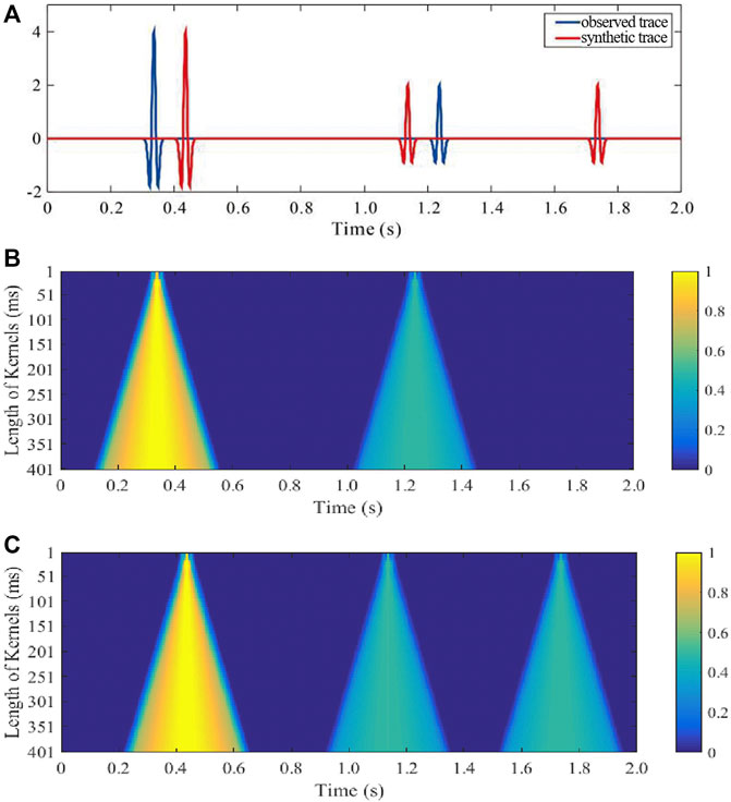
FIGURE 1. Features extracted by different lengths of Gaussian kernels. (A) Observed and synthetic trace. Feature map of the (B) observed trace and (C) synthetic trace with nw = 80 and lnw = 401 ms.
2.2 Dynamic data matching and reliability constraint
After extracting the features, a feature vector consisting of the multiple features of each time sample can be expressed as
where
Thus,
where
Figure 2 shows the feature distances between the traces shown in Figure 1A. The minimal feature distances of the first two events between the synthetic and observed trace are located at the time range of the first two events in the observed trace (red box in Figure 2), indicating that the synthetic events that are cycle-skipped to the observed events have been correctly determined. Incorrect matching occurs between the third event of the synthetic trace and the second event of the observed trace (yellow box in Figure 2). Thus, a constraint that evaluates the reliability of dynamic matching was needed. We constrained the dynamic matching by attenuating the amplitude of synthetic time samples according to |Δt|. Therefore, the intermediate synthetic data generated from the original synthetic data after dynamic data matching and reliability evaluation can be expressed as
where
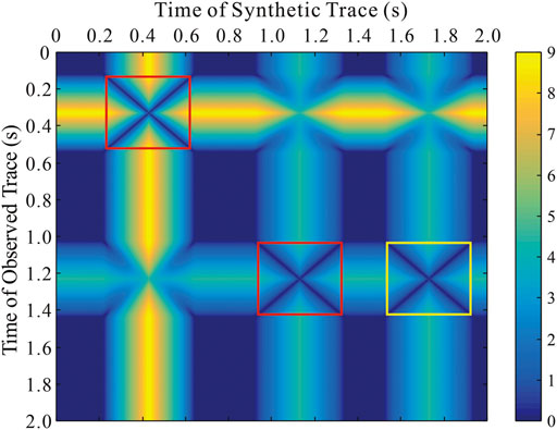
FIGURE 2. Feature distances of the traces shown in Figure 1A.
Figure 3 indicates that the larger the value of |Δt|, the lower the reliability of dynamic matching; the larger the value of γ, the stronger the amplitude attenuation of
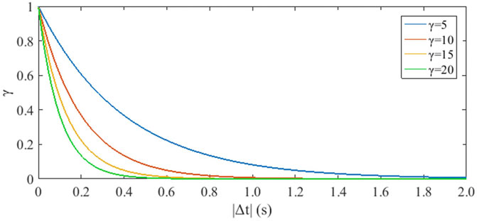
FIGURE 3. Curves of amplitude attenuation to the synthetic time samples with different γ and |Δt|.
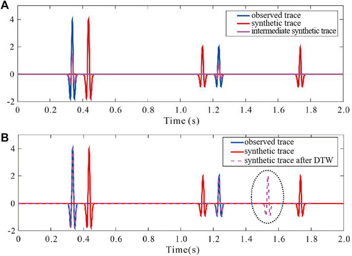
FIGURE 4. Comparison of convolution-based dynamic matching and DTW. The result for (A) convolution-based dynamic matching (γ = 5) and (B) DTW of the waveforms shown in Figure 1A.
2.3 DCFWI
After dynamic matching, the amplitude of some of the time samples in the intermediate synthetic trace were attenuated artificially, which caused the amplitude information of the intermediate synthetic data to be incorrect. In order to weaken the interference of incorrect amplitude and emphasize that the phase information is non-linearly, weaker FWI based on dynamic data matching of convolutional wavefields (DCFWI) uses the global-correlation misfit function as an alternative to the least-squares misfit function (Choi and Alkhalifah, 2012):
where J denotes the misfit function. According to the adjoint state method, the gradient can be expressed as
where v denotes the velocity of the subsurface media. λ represents the adjoint source and is expressed as
Therefore, the gradient in the time domain can be simplified to
where
For a preliminary comparison of DCFWI and standard FWI, we designed two horizontal layered velocity models as the true (Figure 5A) and initial (Figure 5B) models, respectively. The model size was 200 × 200, with a space interval in each direction (distance and depth) of 10 m. Each grid point at surface acts as a receiver. The dominant Ricker wavelet frequency was 20 Hz, and the frequencies below 10 Hz were filtered out to generate data lacking low frequencies. An encoded multi-source containing 15 single shots was used as the source. Figure 6A shows that the waveforms of the observed and synthetic trace are much more complex than the traces shown in Figure 1A, and that the convolution-based dynamic matching methods still move the synthetic events to successfully match the correct observed event under the complex situation. Figures 6B, C show the feature maps of the traces shown in Figure 6A. The illumination of the feature maps shows that the direct and reflection waves were accurately captured by convolutional kernels. The distances between the trace shown in Figure 6A was plotted (Figure 6D) to search for the optimally matched pairs of events. Figure 7A shows the gradient calculated by standard FWI. Due to incorrect matching of waveforms, the velocity from 0.5 to 1.0 km in depth could not be updated. Figure 7B shows the gradient calculated by DCFWI. The velocity from 0 to 1.0 km in depth could be updated more evenly after matching the correct events and attenuating the mismatched synthetic events. Thus, this numerical test preliminarily verified the feasibility of DCFWI. This numerical test aims to demonstrate the ability to mitigate the interference of cycle-skipped events on gradients by DCFWI. However, the velocity variation in depth direction of the model shown in Figure 5 is violent. In order to update this initial model and obtain a desired final inverted result, a method-like reflection waveform inversion (RWI) was needed to remove the high-frequency migration components from the sensitivity kernel and construct a model with low wavenumber for standard FWI. However, this is beyond the scope of this paper.

FIGURE 5. Designed velocity model for comparing standard FWI and DCFWI. (A) True and (B) initial velocity model.
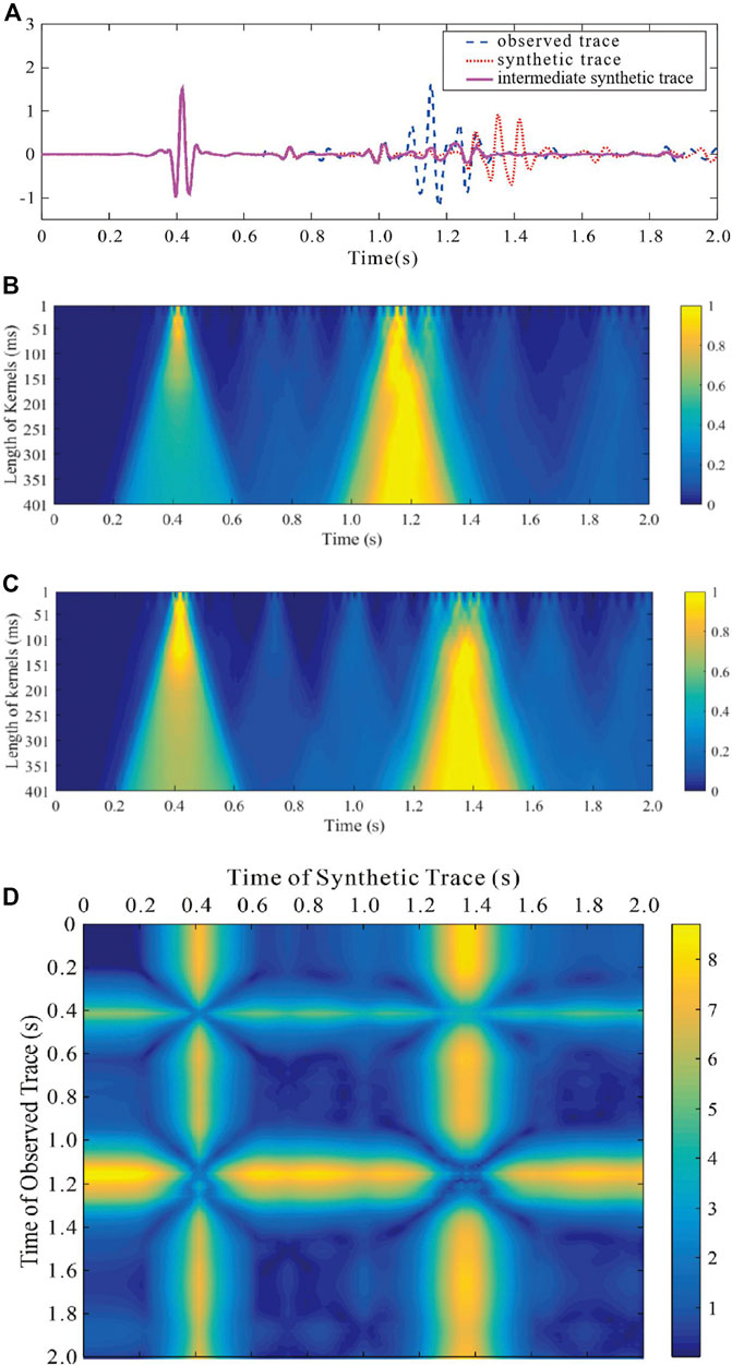
FIGURE 6. Feature maps and distances of complex traces. (A) Comparison of complex traces from encoded multi-source based on the model shown in Figure 5. Feature maps of the (B) observed and (C) synthetic trace. (D) Distances of the traces shown in (A).

FIGURE 7. Gradient comparison based on the velocity model shown in Figure 5. Gradient of (A) standard FWI and (B) DCFWI.
2.4 Convergence and optimal parameter selection of DCFWI
To demonstrate the improved convergence of DCFWI to standard FWI and discuss the optimal parameter selection scheme, we compared the curves of the misfit function derived from a designed velocity model (Figure 8A). The model size was 69 × 192 with a space interval in each direction (distance and depth) of 10 m. The background velocity increased linearly when the minimal velocity was 1.5 km/s and the maximal velocity was 4.0 km/s, and a rectangle-shaped body located in the middle of the model at a velocity of 4.0 km/s. We linearly changed the maximal velocity from 2.5 km/s to 8.0 km/s of the background model to produce a group of initial models to plot the misfit function curves. Two sources with Ricker wavelets were located at the first and end grid points at a depth of 0 km, and 192 receivers were distributed evenly with a space interval of 10 m at a depth of 0 km. The dominant frequency of the Ricker wavelets was 20 Hz, and frequencies below 10 Hz were filtered out to generate data without low frequencies. Standard FWI was performed with the correlation-based misfit function. Figure 8B shows the curve of standard FWI; there were three local minima except for the global minimum— two local minima near the global minimum especially indicated that standard FWI requires an accurate initial model to obtain good inverted results.
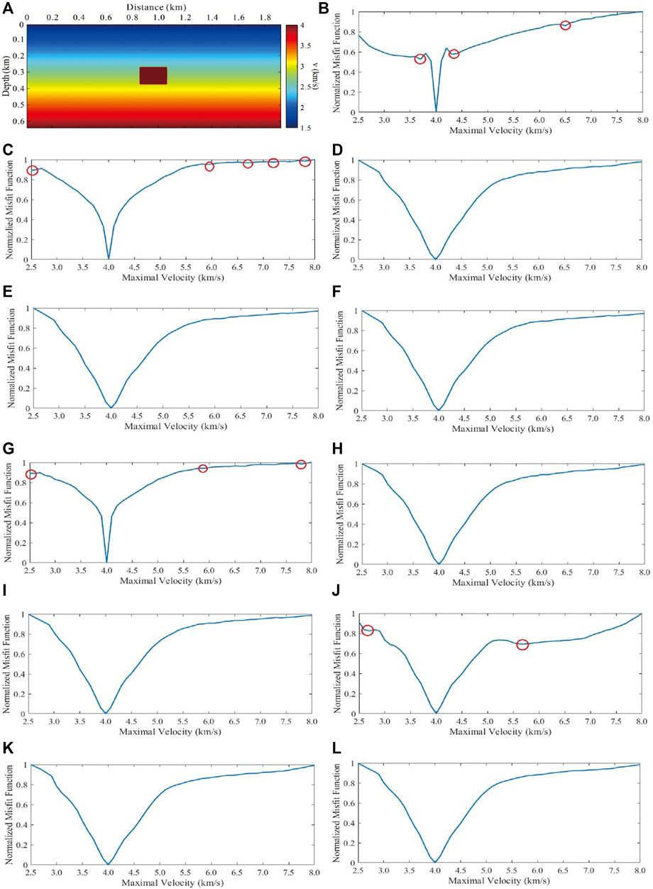
FIGURE 8. Curves of standard FWI and DCFWI with different combinations of parameters based on a designed velocity model, where red circles indicate local minima. (A) Designed velocity model. Curves of (B) standard FWI and DCFWI with (C) nw = 20, ln w= 21 ms, γ = 20; (D) nw = 20, lnw = 101 ms, γ=20; (E) nw = 20, lnw = 201 ms, γ = 20; (F) nw = 20, lnw = 401 ms, γ = 20; (G) nw = 2, lnw = 401 ms, γ = 20; (H) nw = 10, lnw = 401 ms, γ = 20; (I) nw = 40, lnw = 401 ms, γ = 20; (J) nw = 20, lnw = 401 ms, γ = 5; (K) nw = 20, lnw = 401 ms, γ = 10; (L) nw = 20, lnw = 401 ms, γ = 15.
Figures 8C–F show the curve of DCFWI with nw = 20, γ = 20, and lnw = 21 ms, 101 ms, 201 ms, and 401 ms, respectively. Despite its convexity, the curve shown in Figure 8C was better than the curve shown in Figure 8B in the near global minimum regions. Five local minima still appeared where there were large differences between the initial and actual velocity model. However, the curves shown in Figures 8D–F are smooth, which indicates better convergence. The curves of DCFWI with the same nw, γ, and different lnw show that we selected the larger lnw we selected behaved better than a smaller lnw in convergence. The larger lnw extracted features for each time sample in a larger time range, which improved the dynamic matching between two cycle-skipped events in large travel-time differences. Thus, the selection of parameter lnw should at least be larger than the time lapse of a wavelet.
Figures 8F–I show the curve of DCFWI with lnw = 401 ms, γ = 20, and nw = 2, 10, 20, and 40, respectively. Although the convexity of the curve shown in Figure 8G is better than that of the curve shown in Figure 8B in the near global minimum regions, three local minima still appear where there are large differences between the initial and actual velocity model. However, the curves shown in Figures 8F, H, I are smooth, indicating better convergence. The curves of DCFWI with the same lnw, γ, and different nw show that the larger nw we selected behaved better than a smaller nw in convergence. The larger nw indicated that we used more Gaussian kernels for feature extraction. The more kernels we used, the more accurate was the dynamic matching, especially for complex seismic signals. Thus, the selection of parameter nw should be large. In addition, if we use too many kernels to extract features, the accuracy of dynamic matching will not further improve and the computational cost will increase significantly.
Figures 8F, J–L show the DCFWI curve with lnw = 401 ms, nw = 20, and γ = 5, 10, 15, and 20, respectively. Although the convexity of the curve shown in Figure 8J is better than that of the curve shown in Figure 8B in the near global minimum regions, two local minima still appear where there are large differences between the initial and actual velocity model. However, the curves shown in Figures 8F, K, L are smooth, indicating better convergence. The curves of DCFWI with the same lnw and nw and different γ show that the larger γ we selected behaved better than a smaller γ in convergence. The larger γ indicates a stricter constraint for the reliability of dynamic matching, and that some synthetic events that are cycle-skipped to the observed events with large travel-time differences will be completely attenuated to reduce the interference on the gradient of these mismatched events. Thus, the selection of parameter γ should be large. In addition, if we choose too large a value for γ, it indicates an extremely strict constraint for dynamic matching. Some synthetic and observed events with small travel-time differences will also be completely attenuated, causing FWI to lack sufficient valid data to update the initial model.
3 Numerical tests
We tested DCFWI on the Marmousi model (Figure 9A). The grid dimensions were 138 × 384, and the grid spacing in each dimension was 24 m. Each grid point on the surface acted as a receiver, and 50 sources were evenly distributed on the surface. The Ricker wavelet with a peak frequency of 8 Hz was used as a source; to simulate the situation when the observed data lacked low frequencies, a 4 Hz high-pass filter was applied to the wavelet. The total recording time was 6 s with a sampling rate of 0.002 s. The finite-difference method for the acoustic wave equation with PML absorbing boundary was used for seismic wavefield modeling. The L-BFGS optimal algorithm was used for iterating models. The gradient calculated by Eq. 10 was not preconditioned during the inversion process. The velocity of the initial model linearly increased (Figure 9B). We performed standard FWI and DCFWI with multi-scale strategy. The number of iterations in both low frequency (0–7 Hz) and high frequency bands (above 7 Hz) was 350. Although the inversion in the low frequency band was the first step, the lack of sufficiently low frequencies in the observed data caused cycle skipping, resulting in obvious artifacts in the shallow layers of standard FWI (Figure 9C). DCFWI behaved better, correctly recovering the long-wavelength components of the true model (Figure 9D). However, DCFWI artificially attenuated the amplitude of some events in synthetic data, which caused part of the information for further improving the inverted precision to always be absent from the synthetic data. Therefore, DCFWI provided an accurate initial model for standard FWI to obtain the final high precision inverted result. The final inverted model of standard FWI started from the initial model shown in Figure 9C is much deviated from the true model, and the artifacts accumulated during standard FWI (Figure 9E). The final inverted model started from the initial model provided by DCFWI is close to the true model (Figure 9F).
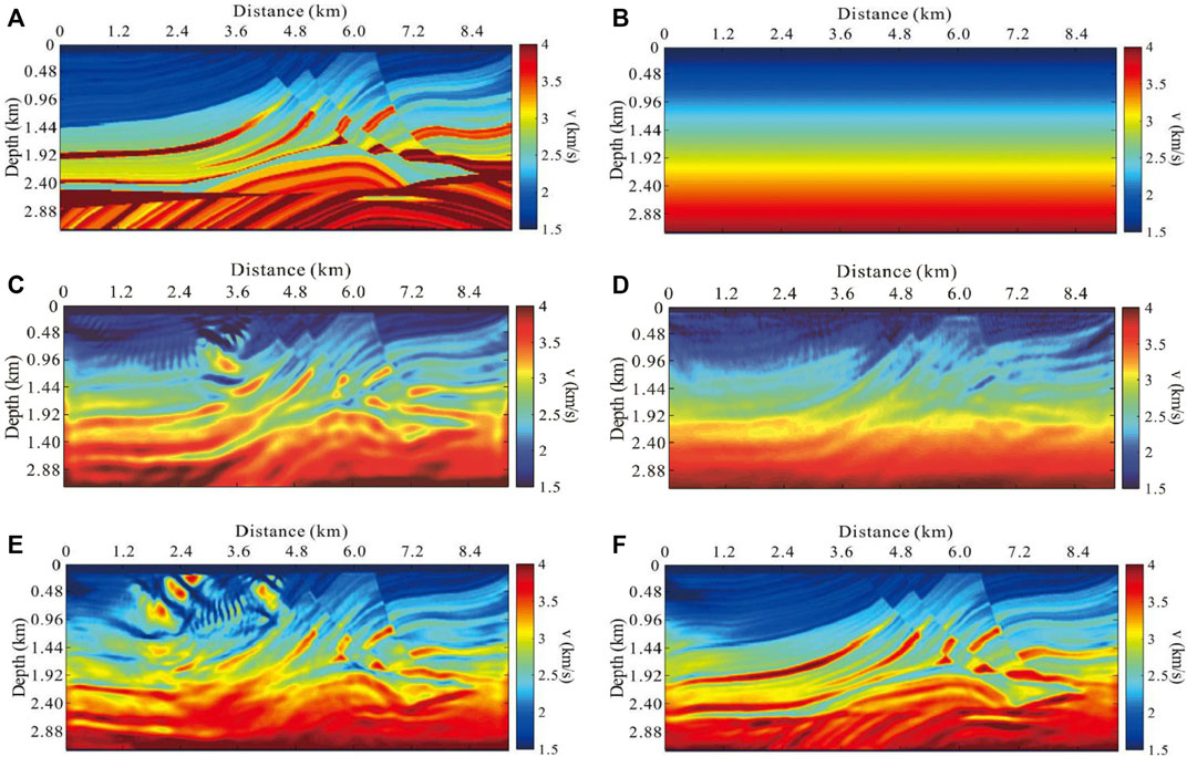
FIGURE 9. Inversion tests. (A) Marmousi model. (B) Initial model (background model); inverted model of (C) standard FWI and (D) DCFWI (nw = 20, lnw = 401 ms, and γ = 20) in a low-frequency band. Final inverted model (E) starts from the velocity shown in (C) and (F) starts from the velocity shown in (D).
The Marmousi model can be divided into a background model (Figure 9B) and a perturbation model (Figure 10A). By continuously changing the maximal velocity of the former and the percentage of the latter, a series of new models can be produced. After calculating the misfit function of FWI on these models, a contour indicating the convergence of FWI can be plotted (Luo and Wu, 2015). The global minimum appears when the percentage of the perturbation model is 100% and the maximal velocity of the background model is 4.0 km/s. Standard FWI cannot tackle the influence of cycle-skipping and will result in incorrect inverted models (local minima) compared to the true velocity model, especially when the initial models differed greatly from the true velocity model (Figure 10B). Figure 10C shows the contour of DCFWI. Although the low frequencies of observed data are filtered out, and some of the initial models are much more different from the true model, DCFWI still has a strong capability for converging and obtaining a correct inverted result (global minimum).
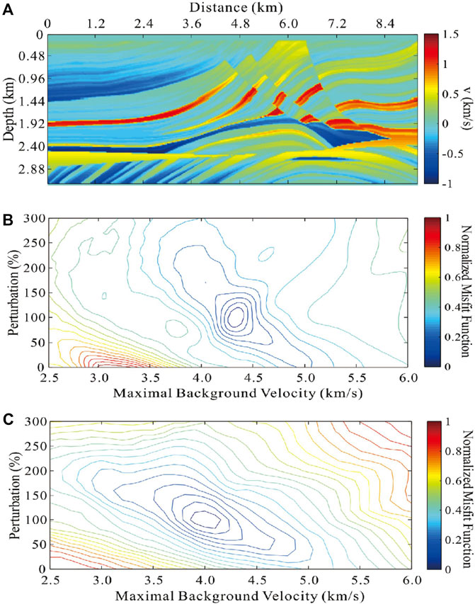
FIGURE 10. Convergence comparison between standard FWI and DCFWI. (A) Perturbation model. Contour of (B) standard FWI and (C) DCFWI.
The random noise-contained observed data with a SNR of −2.6 was used for anti-noise testing of DCFWI. The features extracted by Gaussian convolutional kernels suppress random noise in signals, so that relatively accurate features can be obtained. In addition, the global-correlation misfit function has the ability to decrease the impact of noise. Therefore, a relatively accurate inverted model was obtained by DCFWI, when the observed data lacked low frequencies and was also contaminated by noise (Figure 11).
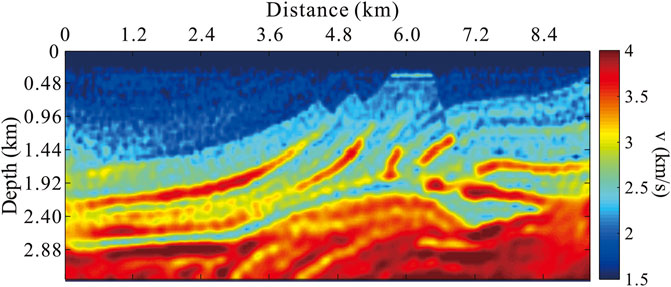
FIGURE 11. Inverted model of DCFWI from noise-contained observed data.
4 Conclusion
In this paper, we propose that features of each time sample extracted by different convolutional kernels can be used to dynamically match synthetic events with the correct observed event. The use of multiple lengths of Gaussian kernels to obtain the features centered on each time sample can improve the accuracy of dynamic matching. Amplitude attenuation according to travel-time differences is an effective constraint for evaluating the reliability of dynamic matching, which produces the intermediate synthetic data that regulates inversion in correct directions. We discuss and conclude the optimal selections of the parameters when DCFWI is performed. Numerical tests on the Marmousi model demonstrate the feasibility of DCFWI for solving the cycle skipping problem and mitigating noise interference. In the future, we will test the application effect of the DCFWI method in field marine seismic data.
Data availability statement
The datasets presented in this study can be obtained by contacting the corresponding author directly.
Author contributions
Methodology, LZ and SD; manuscript writing, SD; programming and software, PZ and YH; funding and review, LH and LZ; investigation and validation, PZ.
Funding
This study was supported financially by the Fundamental Research Funds for the Central Institutes of China (CKSF2023307/YT and CKSF2023316/YT), the National Natural Science Foundation of China (Nos 42130805, 42004106, and 42104116), and the Natural Science Foundation of Jilin Province (No. YDZJ202101ZYTS020).
Acknowledgments
This work was carried out in part using computing resources at Jilin University.
Conflict of interest
The authors declare that the research was conducted in the absence of any commercial or financial relationships that could be construed as a potential conflict of interest.
Publisher’s note
All claims expressed in this article are solely those of the authors and do not necessarily represent those of their affiliated organizations, or those of the publisher, the editors, and the reviewers. Any product that may be evaluated in this article, or claim that may be made by its manufacturer, is not guaranteed or endorsed by the publisher.
References
Barnier, G., Biondi, E., and Biondi, B. (2018). Full-waveform inversion by model extension. Anaheim, CA: SEG Technical Program Expanded Abstracts, 1183–1187. doi:10.1190/segam2018-2998613.1
Bunks, C., Saleck, F. M., Zaleski, S., and Chavent, G. (1995). Multiscale seismic waveform inversion. Geophysics 60, 1457–1473. doi:10.1190/1.1443880
Chen, F., Peter, D., and Ravasi, M. (2022). Cycle-skipping mitigation using misfit measurements based on differentiable dynamic time warping. Geophysics 87, R325–R335. doi:10.1190/geo2021-0598.1
Chi, B., Dong, L., and Liu, Y. (2014). Full waveform inversion method using envelope objective function without low frequency data. J. Appl. Geophys. 109, 36–46. doi:10.1016/j.jappgeo.2014.07.010
Choi, Y., and Alkhalifah, T. (2012). Application of multi-source waveform inversion to marine streamer data using the global correlation norm. Geophys. Prospect. 60, 748–758. doi:10.1111/j.1365-2478.2012.01079.x
Dong, X., Li, Y., and Yang, B. (2019). Desert low-frequency noise suppression by using adaptive DnCNNs based on the determination of high-order statistic. Geophys. J. Int. 219 (2), 1281–1299. doi:10.1093/gji/ggz363
Dong, X., Lin, J., Lu, S., Wang, H., and Li, Y. (2022a). Multiscale spatial attention network for seismic data denoising. IEEE Trans. Geosci. Remote. Sens. 60, 1–17. doi:10.1109/TGRS.2022.3178212
Dong, X., Lin, J., Lu, S., Huang, X., Wang, H., and Li, Y. (2022b). Seismic shot gather denoising by using a supervised-deep-learning method with weak dependence on real noise data: A solution to the lack of real noise data. Surv. Geophys. 43 (5), 1363–1394. doi:10.1007/s10712-022-09702-7
Dong, S., Han, L., Hu, Y., and Yin, Y. (2020). Full waveform inversion based on a local traveltime correction and zero-mean cross-correlation-based misfit function. Acta Geophys. 68, 29–50. doi:10.1007/s11600-019-00388-x
Dong, X., Zhong, T., and Li, Y. (2020). New suppression technology for low-frequency noise in desert region:the improved robust principal component analysis based on prediction of neural network. IEEE Trans. Geosci. Remote. Sens. 58 (7), 4680–4690. doi:10.1109/TGRS.2020.2966054
Guo, P., Visser, G., and Saygin, E. (2020). Bayesian trans-dimensional full waveform inversion: Synthetic and field data application. Geophys. J. Int. 222 (1), 610–627. doi:10.1093/gji/ggaa201
Guo, P., Singh, S., Vaddineni, V., Grevemeyer, I., and Saygin, E. (2022). Lower oceanic crust formed by in situ melt crystallization revealed by seismic layering. Nat. Geosci. 15, 591–596. doi:10.1038/s41561-022-00963-w
Han, J., and Van, M. (2015). Microseismic and seismic denoising via ensemble empirical mode decomposition and adaptive thresholding. Geophysics 80 (6), KS69–KS80. doi:10.1190/geo2014-0423.1
Huang, G., Nammour, R., and Symes, W. (2017). Full-waveform inversion via source-receiver extension. Geophysics 82, R153–R171. doi:10.1190/geo2016-0301.1
Huang, G., Ramos-Martínez, J., Yang, Y., and Chemingui, N. (2021). FWI in extended domain using time-warping. Anaheim, CA: SEG Technical Program Expanded Abstracts, 817–821. doi:10.1190/segam2021-3594800.1
Liu, Y., and Zheng, Z. (2022). Noniterative f-x-y streaming prediction filtering for random noise attenuation on seismic data. IEEE Trans. Geosci. Remote. Sens. 60, 1–9. doi:10.1109/TGRS.2021.3099431
Liu, Y., He, B., Lu, H., Zhang, Z., Xiao, B., and Zheng, Y. (2018). Full intensity waveform inversion. Geophysics 83, R649–R658. doi:10.1190/geo2017-0682.1
Luo, J., and Wu, R.-S. (2015). Seismic envelope inversion: Reduction of local minima and noise resistance. Geophys. Prospect. 63, 597–614. doi:10.1111/1365-2478.12208
Mojica, O. F., and Kukreja, N. (2019). Towards automatically building starting models for full-waveform inversion using global optimization methods: A PSO approach via deap + devito. Anaheim, CA: SEG Technical Program Expanded Abstracts, 5174–5178. doi:10.1190/segam2019-3216316.1
Rizzuti, G., Louboutin, M., Wang, R., and Herrmann, F. J. (2021). A dual formulation of wavefield reconstruction inversion for large-scale seismic inversion. Geophysics 86, R879–R893. doi:10.1190/geo2020-0743.1
Sun, H., and Demanet, L. (2018). Anaheim, CA: SEG Technical Program Expanded Abstracts, 2011–2015. doi:10.1190/segam2018-2997928.1Low-frequency extrapolation with deep learning
Virieux, J., and Operto, S. (2009). An overview of full-waveform inversion in exploration geophysics. Geophysics 74, WCC1–WCC26. doi:10.1190/1.3238367
Wang, M., Xie, Y., Xu, W. Q., Loh, F. C., Xin, K., Chuah, B. L., et al. (2016). Dynamic-warping full-waveform inversion to overcome cycle skipping. Anaheim, CA: SEG Technical Program Expanded Abstracts, 1273–1277. doi:10.1190/segam2016-13855951.1
Yang, J., Li, Y. E., Liu, Y., Wei, Y., and Fu, H. (2020). Mitigating the cycle-skipping of full-waveform inversion by random gradient sampling. Geophysics 85, R493–R507. doi:10.1190/geo2020-0099.1
Yang, T., Chai, X., Nie, W., and Yu, J. (2022). “Deep-learning-based low-frequency reconstruction for full-waveform inversion,” in SEG 2021 Workshop: 4th International Workshop on Mathematical Geophysics: Traditional & Learning, 17–19 December 2021 (SEG Library), 134–137. doi:10.1190/iwmg2021-35.1
Zhang, D., Leeuw, M., and Verschuur, E. (2021). Deep learning-based seismic surface-related multiple adaptive subtraction with synthetic primary labels. Anaheim, CA: SEG Technical Program Expanded Abstracts, 2844–2848. doi:10.1190/segam2021-3584041.1
Keywords: full waveform inversion (FWI), Gaussian convolutional kernels, features extraction, dynamic data matching, optimal matching, travel-time differences constraint
Citation: Zhou L, Dong S, Han L, Zhang P and Hu Y (2023) Full waveform inversion based on dynamic data matching of convolutional wavefields. Front. Earth Sci. 11:1134871. doi: 10.3389/feart.2023.1134871
Received: 31 December 2022; Accepted: 31 March 2023;
Published: 19 April 2023.
Edited by:
Peng Guo, Commonwealth Scientific and Industrial Research Organisation (CSIRO), AustraliaReviewed by:
Bowen Li, Huawei Technologies, ChinaWenyong Pan, Institute of Geology and Geophysics (CAS), China
Copyright © 2023 Zhou, Dong, Han, Zhang and Hu. This is an open-access article distributed under the terms of the Creative Commons Attribution License (CC BY). The use, distribution or reproduction in other forums is permitted, provided the original author(s) and the copyright owner(s) are credited and that the original publication in this journal is cited, in accordance with accepted academic practice. No use, distribution or reproduction is permitted which does not comply with these terms.
*Correspondence: Shiqi Dong, ZHNxMTk5NEAxMjYuY29t