Filtering GRACE temporal gravity field solutions using ensemble empirical mode decomposition approach

Due to the strong noise that exists in GRACE (Gravity Recovery and Climate Experiment) temporal gravity field solutions, geophysical signals are normally drowned which need many effective filtering approaches. Considering the advantage of the ensemble empirical mode decomposition (EEMD) approach, we used the EEMD to filter the noise in this study together with the empirical mode decomposition (EMD) for comparisons. EMD method is a spectrum analysis method, which is very effective for non-stationary signals. EMD process is essentially a means to process non-stationary signals. It has been applied in many fields in recent years. Considering the characteristics of the spherical harmonic coefficient model that the noise level higher with the increasing degree, we divided the gravity field solutions into two parts (degrees 2–28 and degrees 29–60) based on the ratios of the latitude-weighted root mean square (RMS) over the land and ocean signals when adopting different truncated degrees. For the real GRACE solution experiments, the results show that the fitting errors of EEMD approach are always smaller than those of EMD approach, and the mean RMS ratio of EEMD is 3.45, larger than 3.40 of EMD. The simulation results show that the latitude weighted root mean square errors for EEMD approach are smaller than those of EMD, indicating that EEMD can extract the geophysical signals more accurately. Therefore, it is reasonable to conclude that EEMD performs better than EMD for filtering GRACE solutions.

1 Introduction

As the global climate and environmental issues become more serious with the passage of time, more accurate monitoring of land water storage, sea level change, glacial melt, and redistribution of surface mass is important to this problem. The successful GRACE (Gravity Recovery and Climate Experiment) satellite, jointly developed by NASA and DLR, has made it possible to provide highly accurate global gravity field observations, paving the way for the observation of global climate change (Feng, 2013; Lu et al., 2015; Ning et al., 2016). The GRACE plays an important role in the study of regional hydrology (Landerer et al., 2010), ice sheet balance (Velicogna & Wahr, 2013) and ocean mass redistribution (Chambers & Bonin, 2012). And through GRACE, an Earth gravity field map with a spatial resolution of several hundred kilometers and a time resolution of 1 month is provided (Bettadpur et al., 2012; Watkins & Yuan, 2012; Dahle et al., 2013).

The GRACE satellite is subject to a number of factors in its orbit that can cause a certain amount of error in the spherical harmonic (SH) coefficients of the gravity field model it provides, such as satellite orbit error, instrument error, and satellite attitude measurements (Tapley et al., 2004). These errors can have a combined effect on the time-varying Earth’s gravity field model. The mass density of the earth’s surface change seriously affected the time-varying gravity field model inversion. The serious north-south (NS) striping errors in the gravity field inversion is mainly due to the configuration of satellite orbits for the GRACE mission, which can mask the true geophysical signal and be detrimental to the subsequent work, so some filtering methods are needed. Currently commonly used filtering methods can be divided into two categories (Guo et al., 2018). The first type of filtering algorithm is the introduction of filtering factors to reduce the weight of higher order terms in the data processing, which is called spatial filtering and so as to achieve the purpose of removing the striping error, mainly including Gaussian filtering (Wahr et al., 1998), Wiener filtering (Sasgen et al., 2007), Fan filtering (Zhang et al., 2009), and DDK filtering (Kusche et al., 2007; Kusche et al., 2009), etc. However, there are certain limitations of this type of filtering, with the increase of the filtering radius, although the noise is effectively removed, the real signal is also gradually weakened, that is, at the expense of the spatial resolution is sacrificed to achieve the removal of stripe noise (Zhan et al., 2011). The second type of filtering is decorrelation filtering, which uses polynomial fitting to achieve the purpose of decorrelation, including polynomial fitting (PnMm) and sliding window polynomial fitting, such as the commonly used P4M6 (Chen et al., 2007), P4M15 (Chambers et al., 2012), Duan (Duan et al., 2009) and so on. Some scholars also introduced the temporal and spatial filtering, mainly includes empirical orthogonal functions (Schrama et al., 2007; Wouters & Schrama, 2007), the stochastic filter (Wang et al., 2016), multichannel singular spectrum analysis (Guo et al., 2018; Prevost et al., 2019; Wang et al., 2020), and the least square filter (Crowley & Huang, 2020).

Temporal filtering treats the NS striping noise as white/random noise, and it is suggested that this random signal can be identified with the growth of time information (Yi et al., 2022). Nowadays, a combined filtering approach is the preferred choice. The adaptive time-frequency localization analysis approach empirical mode decomposition (EMD) (Huang et al., 1998), was used to post-process the time-varying GRACE gravity field models, demonstrated that EMD can better remove the strong noise with less signal leakage (Huan et al., 2022; Ai et al., 2022). Considering the mode mixing problem existed in EMD approach, an ensemble EMD (EEMD) approach was developed by Wu et al. (2009). In view of the advantage of EEMD approach with respect to EMD, and the good performance of EMD for filtering GRACE gravity field models, here in this study we will try to apply EEMD to extract the geophysical signals from the SH coefficients of GRACE time-varying gravity field models, together with EMD approach for comparisons. The rest of this paper is organized as follows: Section 2 introduces the theories of EEMD and EMD. In Section 3, we describe and analyze the results in the spectrum domain and spatial domain and Section 4 is the simulation experiment, Section 5 is the summary of the results.

2 Methods

In today’s signal processing field, there are many signal processing approaches, such as empirical mode decomposition, variational mode decomposition, local mean decomposition, etc. However, most of the signals we face are non-linear and non-stationary, in order to achieve our desired decomposition effect, we need to use more efficient and convenient analysis approach. EEMD is an adaptive spectrum analysis approach which improved the mode mixing problem on the basis of EMD, has been widely applied in many research fields. For example, global navigation satellite system (GNSS) data processing (Niu et al., 2018), mechanical vibration analysis (Lei et al., 2009), diagnosis of winding faults in a transformer (Mejia-Barron et al., 2017), and so on.

2.1 Empirical mode decomposition approach

Compared with wavelet analysis and other spectral analysis approaches, EMD is more adaptive and convenient to extract the signal information from the noisy time series Figure 1. The main steps of EMD approach are as follows.

(1) Fitting all the maximum and minimum points of the original time series $x\left(t\right)$, and fit the maximum $e_{\max }\left(t\right)$ and minimum envelope $e_{\min }\left(t\right)$ by cubic spline function.

(2) Calculating the average value $m\left(t\right)$ of the upper and lower envelope.

$m\left(t\right)=\frac{e_{\max }\left(t\right)+e_{\min }\left(t\right)}{2},(1)$

(3) Subtracting $m\left(t\right)$ from the original time series $x\left(t\right)$ to get a new time series $h\left(t\right)$,

$h\left(t\right)=x\left(t\right)-m\left(t\right),(2)$

(4) Judging whether $h\left(t\right)$ satisfies the two basic conditions of IMF (Intrinsic Mode Functions), Physically, the necessary condition for defining meaningful instantaneous frequency is that the function is symmetric about the local zero mean value and has the same number of zero-crossing and extreme values. Based on these observations, we propose a class of functions called Intrinsic Mode Functions (IMF). i.e.,: 1) In the entire data segment, the number of extreme points and the number of zero-crossing points must be equal or the difference cannot exceed one at most. 2) At any time, the average value of the upper envelope formed by the local maximum points and the lower envelope formed by the local minimum points is zero, that is, the upper and lower envelopes are locally symmetrical concerning the time axis (Zhang et al., 2017). However, for the actual decomposition process, the second condition is difficult to satisfy and the threshold expression for stopping filtering for each component is as follows:

$SD={\displaystyle \sum }_{t=1}^N\left[\frac{{\left|d_{k+1}\left(t\right)-d_k\left(\mathrm{t}\right)\right|}^2}{d_{k-1}^2\left(t\right)}\right](3)$

where $d_k\left(t\right)$ and $d_{k-1}\left(t\right)$ are two adjacent data sequences in the IMF selection process and $N$ represents the length of time series, $SD$ represents the threshold at which each IMF stops filtering, which is usually taken as a number between 0.2 and 0.3 (Huang et al., 1998). If it is satisfied, set $h\left(t\right)$ as the first IMF component $c_1\left(t\right)$ of the original time series. If not, repeat steps 1 and 2, until it satisfies the two conditions of IMF.

(5) $c_1\left(t\right)$ is separated from the original time series to generate a new series $r\left(t\right)=x\left(t\right)-c_1\left(t\right)$. Repeat the above steps to obtain n IMF components and a residual sequence only when the residual sequence satisfies the monotonic condition.

(6) The original series $x\left(t\right)$ after EMD decomposition can be expressed as follows,

$x\left(t\right)={\displaystyle \sum }_{i=1}^n{c}_i\left(t\right)+r\left(t\right),(4)$

(7) Normally the high-frequency components are recognized as noise, and the remaining components are used to reconstruct the signals.

$s\left(t\right)={\displaystyle \sum }_{i=d}^n{c}_i\left(t\right)+r\left(t\right),(5)$

where d is the boundary point between noise and signal component.

FIGURE 1

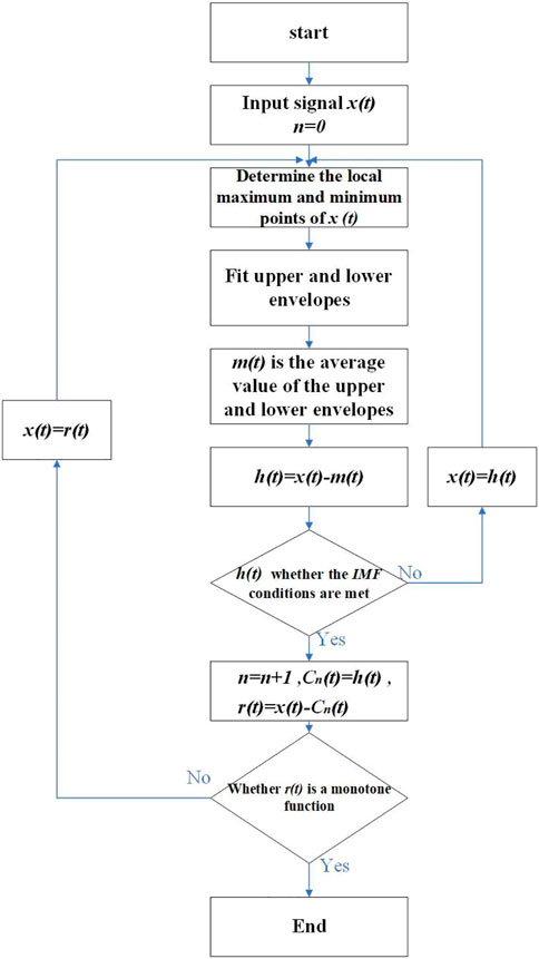
FIGURE 1. The flow chart of empirical mode decomposition approach.

2.2 Ensemble empirical mode decomposition approach

EEMD approach was developed to compensate for the shortcomings of the EMD approach in terms of mode mixing, and can decompose a complex signal into a collection of IMFs based on the local eigentime scales of the signal (Huang et al., 1998). EEMD takes advantage of the unique feature that white noise has a mean value of zero and adds the same white noise to the signal to be analyzed, masking out the noise in the signal itself by adding artificial noise several times to obtain a more accurate upper and lower envelope. The EEMD algorithm improves on the shortcomings of EMD’s confounding modes and perfectly retains its adaptive, orthogonal characteristics. The specific procedures are as follows.

Step 1. Gaussian white noise is added to the original time series $x\left(t\right)$, and $w\left(t\right)$ is determined by the standard deviation of the true signal.

Step 2. The new generated time series $x^{\prime }\left(t\right)=x\left(t\right)+w\left(t\right)$ is decomposed by EMD, resulting in n IMF components $c_i\left(t\right)\left(i=\mathrm{1,2},\cdots ,n\right)$ and the residual component $r\left(t\right)$. The corresponding SH coefficient signal is reconstructed as $s^{\prime }\left(t\right)={\displaystyle \sum }_{i=d}^n{c}_j\left(t\right)+r\left(t\right)$.

Step 3. Repeat steps 1–2 for P times, then the final extracted signals $s\left(t\right)$ is computed by averaging all reconstructed signal $s^{\prime }\left(t\right)$ for P times.

2.3 Ensemble empirical mode decomposition for filtering GRACE time-varying gravity field models

The RL06 version of the earth gravity field models developed by CSR (the Space Research Center) are adopted, whose SH coefficients are up to degree and order (d/o) 60. Considering that the noise increases with the increasing degree, to better filter the noise of different degree SH coefficients, we decide to divide the SH coefficients into two parts (d/o 2–28 and 29–60) and filter using differ strategies. Noting that the boundary degree 28 is determined by computing the latitude weighted RMS of land and ocean (Chen et al., 2007) for all degree SH coefficients (Figure 2).

FIGURE 2

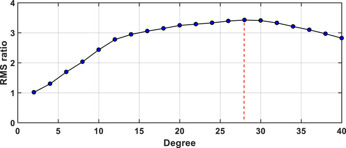
FIGURE 2. The mean RMS_ ratios with the increasing degree (no filtering) over April 2002 to August 2016.

The specific filtering procedures are presented as follows: 1) Removing the mean field; 2) Interpolating the missing months using cubic spline; 3) Improving the endpoint effect using an autoregressive model to extend the coefficient sequence forward and backward to three maximum points and three minimum points (Guo et al., 2016); 4) Filtering the stripe errors using DDK7 approach; 5) Applying EEMD for filtering the time-varying gravity field models, for the d/o 2–28 SH coefficients, all IMFs whose period larger than 0.4 are retained, and for d/o 29–60, all IMFs whose period larger than 0.8 are used to reconstruct the signals. Considering the computation efficiency and accuracy for extracting signals, the decomposition times of degrees 2–28 is 10 times and the number of decomposition of degrees 29–60 is 30 times. Noting that for the real GRACE time series, the true signal is not known, thus we use the reconstructed SH signals by EMD approach to generate the added noise. 6) Reconstruct the filtered SH coefficients, and convert into global mass change in terms of equivalent water height (EWH). The processing flow for filtering the GRACE SH coefficient is shown in Figure 3.

FIGURE 3

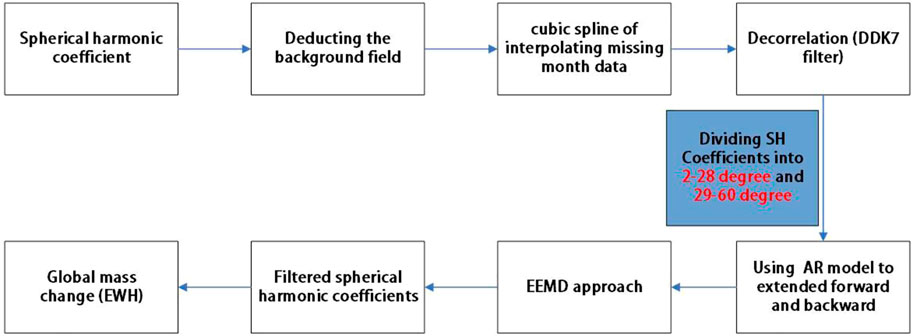
FIGURE 3. The flowchart of EEMD for filtering GRACE models.

3 Results and analysis

3.1 Comparison of filtered SH coefficients

We adopted the CSR RL06 SH coefficients (d/o 60) covering the period from April 2002 to August 2016, with 17 missing months, representing 9.8% of the total months. Following the processing procedures presented in Section 2, we perform the EEMD and EMD for filtering GRACE SH coefficients. Normally the signal is low-frequency, the noise has a relative high frequency. Besides, it is hardly to filter the strong noise accurately when just use the simple filtering approach (Guo et al., 2018; Shen et al., 2021), therefore a combined filtering approach is preferred. Considering the advantage of DDK filter (Prevost et al., 2019) and applicability of EEMD approach, we determined to use the combined filtering, which adopted the decorrelation filtering (i.e., DDK7) approach for eliminating the stripe noise, and EEMD for removing the remained high-frequency errors.

Many previous studies concluded that the low-degrees part of the gravity field model contains less noise, mainly the real geophysical signals, while the high-degrees part contains more noise and the real signal is relatively small. Therefore, here we take two coefficients C_3,2 and C_60,59, for example,. The power spectrum analysis approach is used to judge whether the component belongs to signal or noise (Huan et al., 2022). The highest point of power whose period corresponding is the main period of the IMF components (Shu et al., 2007). Figure 4 shows the IMF components of the two SH coefficients derived by EEMD and EMD. For the IMF components, IMF2-IMF4 are related to the dominant semiannual and annual periods, IMF5-IMF6 mainly 2.1–2.5 years period components and IMF7-IMF8 mainly related to the long-term trend (Schmidt et al., 2008). The reconstructed SH signal by EEMD and EMD approaches are presented in Figure 5. It can be seen that the amplitude fluctuation range of the reconstructed coefficients is very similar just with slight differences.

FIGURE 4

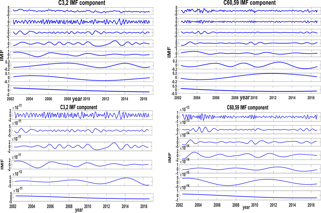
FIGURE 4. IMF components for C_3,2 and C_60,59 coefficients (Up: EEMD; Bottom: EMD).

FIGURE 5

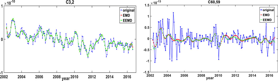
FIGURE 5. Comparison of coefficient reconstructions for C_3,2 (Left) and C_60,59 (Right).

In order to test the performances of EEMD approach with respect to EMD, we calculated the fitting errors of SH coefficients by two approaches as follows,

$\sigma =\sqrt{\frac{1}{N}{\displaystyle \sum }_{t=1}^N\left(x(t)-s(t){)}^2\right.,}(6)$

where $\sigma$ represents the fitting error, $s\left(t\right)$ represents the reconstructed SH signals filtered by EMD and EEMD, $x\left(t\right)$ is the original SH coefficients, and $N$ represents the length of each SH coefficient series. The fitting errors of EEMD are 8.3384e-12 and 2.8451e-12 for C_3,2 and C_60,59 coefficients, smaller than 8.4614e-12 and 2.8463e-12 for EMD approach, respectively. Figure 6 presents all the fitting errors of all SH coefficients, we can conclude that the fitting error of EEMD is almost smaller than that of EMD regardless of low or high degree part, indicating that EEMD can extract more information of original SH coefficients than EMD. In order to verify our results more precisely, a comprehensive analysis is carried out in Section 3.2.

FIGURE 6

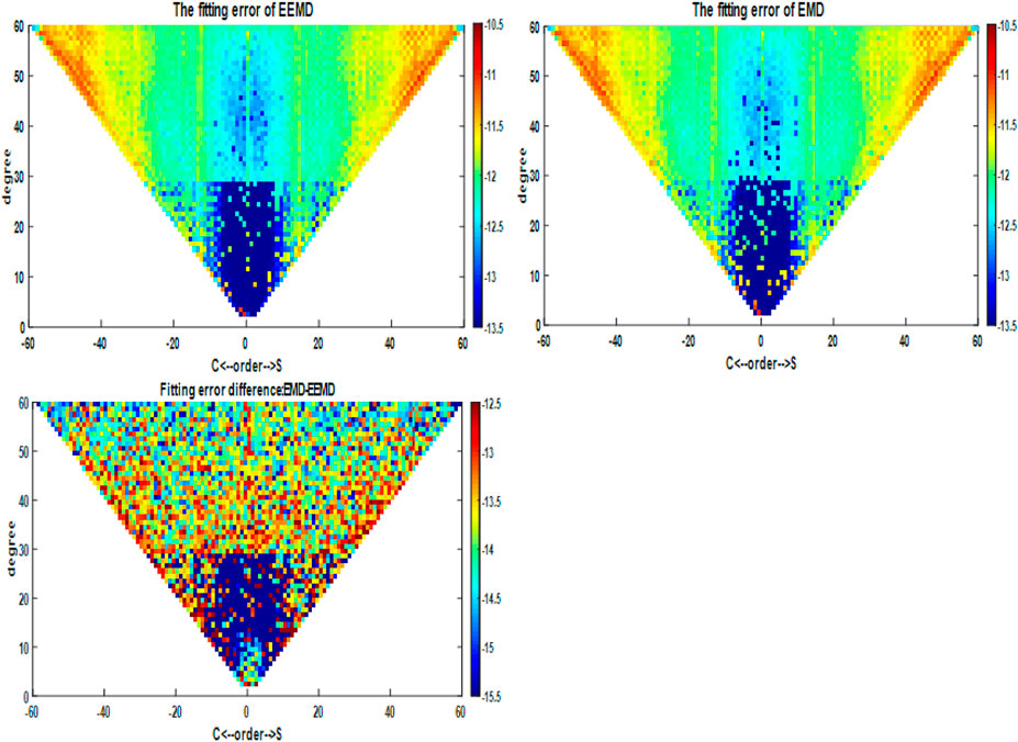
FIGURE 6. The fitting errors of GRACE SH coefficients after filtering by EMD and EEMD and their differences (in log10).

3.2 Global mass change comparison

To further verify the advantages of EEMD approach in extracting the geophysical signal from GRACE SH coefficients, we convert the reconstructed SH signals by EEMD and EMD to EWH in $1^{\circ }\times 1^{\circ }$ grids. In this section we randomly select 2 months May 2013 and January 2016, for example,. Figure 7 shows the global mass changes in May 2013 and January 2016. From Figure 7, we can find that the NS stripe errors are suppressing significantly after DDK7, however, some noise remained, which are removed by EMD and EEMD approaches. Noting that after EEMD filtering, the general shape and amplitude of the original signal in some areas are well preserved, such as Greenland, Arctic, and Antarctic. To conduct a more accurate signal quality analysis, we selected the Greenland as a case study, as shown in Figure 8. We compared the EEMD-filtered signal with the EMD and the Gaussian method. It is reasonable to conclude that EEMD and EMD methods can effectively improve the leakage error compared with the Gaussian method. And the leakage error of EEMD filtered signal is smaller than that of EMD filtered signal and the reserved signal is stronger.

FIGURE 7

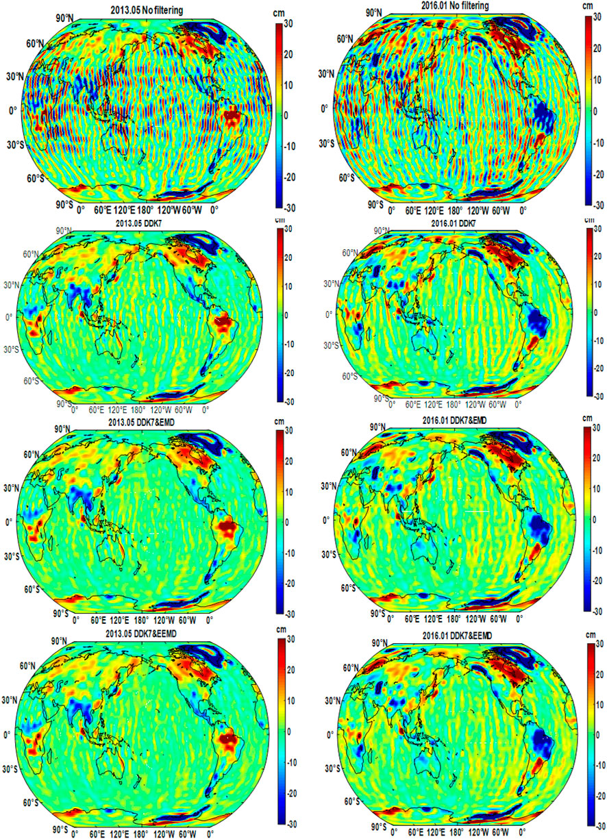
FIGURE 7. Global mass changes in May 2013 and January 2016 (Row 1: No filtering; Row 2: DDK7; Row 3: EMD; Row 4: EEMD).

FIGURE 8

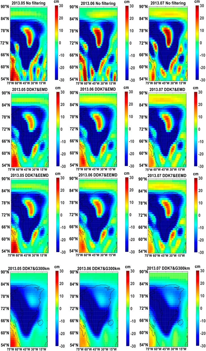
FIGURE 8. EWH map in Greenland after EEMD, EMD, Gaussian smoothing 300 km (G300 km) together with DDK7 and No filtering.

To evaluate the filtering efficiency of EEMD and EMD, we used the ratio of latitude weighted RMS of land and oceans. It is mainly based on the fact that the surface mass of the whole land varies more than the oceans, in addition to the $C_{20}$ term, the variability ratio is the ratio of latitudinal weighted RMS values on land and ocean signals (Chen et al., 2006). To reduce the leakage of signals from land, we use a 300 km buffer zone.

$RM{S}_{ratio}=\frac{RMS\left(MAS{S}_{land}+Err\right)}{RMS\left(MAS{S}_{ocean}+Err\right)},(7)$

where $MAS{S}_{land}\mathrm{a}\mathrm{n}\mathrm{d}MAS{S}_{ocean}$ represent the signals on land and ocean, respectively, $Err$ is the noise.

Table 1 shows the RMS_ratios of EMD and EEMD filtering are 4.74 and 4.53, 4.65, and 4.45 for May 2013 and January 2016, respectively. As shown in Figure 9, all the RMS_ratios of EEMD approach are almost larger than those of EMD. One thing should be mentioned is that we further present the RMS_ratios which not done the modification of endpoint effect in Figure 9, we can find that the corresponding results can better show the well performance of EEMD for filtering the noise. Noting that before improving the endpoint effect, there exist 128 months RMS_ratios of EEMD method which are higher than EMD, and 132 months after improved the endpoint effect. The mean RMS_ratio of EEMD is 3.45 and the EMD is 3.40, which reflects the noise filtering effect of EEMD from another perspective. In all, we can conclude that EEMD performs better in filtering the noise and preserving the geophysical signals than EMD.

TABLE 1

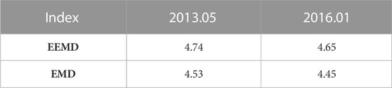
TABLE 1. The RMS_ratio of EMD and EEMD approach for May 2013 and January 2016.

FIGURE 9

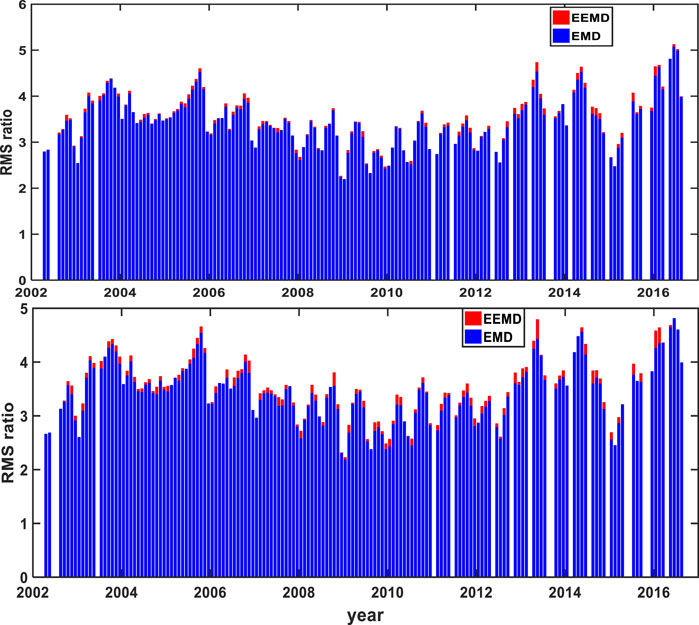
FIGURE 9. The RMS_ratios of all available months from April 2002 to August 2016 by EEMD and EMD (Up: Improving the endpoint effect) and (Bottom: No improving the endpoint effect).

4 Simulation experiments

Though we have validated the advantage of EEMD for filtering the noise and extracting the geophysical signals from GRACE SH coefficients, the simulation experiments are also performed in this study. The CSR RL06 Mascon gridded data are converted to SH coefficients and SH coefficients are up to degree and order (d/o) 60, which is used as the true SH signals. To simulate the real GRACE type noise, we generated the noise from the time-varying gravity field model by DDK7 & EMD filtering, similar to Vishwakarma et al. (2016). Then the noise was added to the true signals to generate the noisy GRACE SH coefficients. Here we take March 2008 as an example to show the global mass changes extracted by EEMD, EMD and Gaussian smoothing 300 km combined with DDK7 filtering approaches in Figure 10. It is obviously to find that the EEMD and EMD approaches can both better filtering the noise with less signal leakage than Gaussian smoothing 300 km.

FIGURE 10

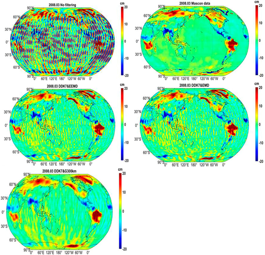
FIGURE 10. Global mass changes extracted by EEMD, EMD, Gaussian smoothing 300 km (G300 km) approaches together with DDK7 filter in March 2008.

To evaluate the quality of extracted signals, we use the latitude weighted root mean squared errors (RMSE) of global mass change differences between true (Mascon) signal and extracted signal by EEMD, EMD and Gaussian smoothing 300 km (Wang et al., 2020), which are calculated as follows,

$RMSE\left(\mathrm{\Omega }\right)=\sqrt{\frac{{\displaystyle \sum }_{\forall i\in \mathrm{\Omega }}\left(\Delta {v_i}^2.\cos {\phi }_i\right)}{{\displaystyle \sum }_{\forall i\in \mathrm{\Omega }}\cos {\phi }_i},}(8)$

where $\Delta v_i$ represents the differences between the true (Mascon) signals and the reconstructed signals, ${\phi }_i$ is the corresponding latitude, $\mathrm{\Omega }$ represents a spatial range and can be global or regional. And all grids within $\mathrm{\Omega }$ are summed based on their area weights reflected by latitudes.

The relative improvement percentage (IMP) of spatial RMSE of EEMD with respect to EMD and Gaussian methods is calculated by,

$IM{P}_{\mathrm{E}}=\frac{{\mathrm{R}\mathrm{M}\mathrm{S}\mathrm{E}}_{EMD}-{\mathrm{R}\mathrm{M}\mathrm{S}\mathrm{E}}_{EEMD}}{{\mathrm{R}\mathrm{M}\mathrm{S}\mathrm{E}}_{EMD}}\times 100\%(9)$

$IM{P}_{\mathrm{G}}=\frac{{\mathrm{R}\mathrm{M}\mathrm{S}\mathrm{E}}_{Gaussian}-{\mathrm{R}\mathrm{M}\mathrm{S}\mathrm{E}}_{EEMD}}{{\mathrm{R}\mathrm{M}\mathrm{S}\mathrm{E}}_{Gaussian}}\times 100\%(10)$

Here we compute the spatial RMSEs of five selected global and regional areas including global, ocean, land, Amazon and Yangtze basins. Figure 11 shows the spatial mean RMSEs of all available months for five selected regions over April 2002 to August 2016 and the corresponding IMPs. It is clearly to find that all the spatial RMSEs of EEMD are smaller than EMD and 300 km Gaussian smoothing approaches, and the relative improvements of EEMD with respect to 300 km Gaussian smoothing are more significant than those of EMD approach for five selected regions, which indicate that EEMD can extract the geophysical signals more accurately than EMD and 300 km Gaussian smoothing approaches. Besides, we further compute the mean mass changes over four regions (Land, Ocean, Amazon and Yangtze) and shown in Figure 12. The corresponding RMSEs of three filtering approaches in terms of the mean mass changes are presented in Table 2. Through the simulation experiments, we can draw the conclusion that EEMD can extract closer geophysical signals than EMD and 300 km Gaussian smoothing approaches.

FIGURE 11

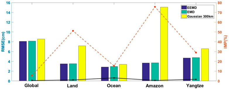
FIGURE 11. The spatial mean RMSEs of EEMD, EMD and Gaussian 300 km for all available months over April 2002 to August 2016 in five selected global and regional areas and the corresponding IMPs (red dotted line: EEMD is relative to Gaussian; black line: EEMD is relative to EMD).

FIGURE 12

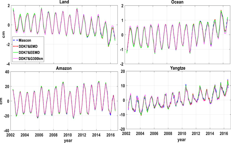
FIGURE 12. Mean mass change series of three filtering approaches in four regions over April 2002 to August 2016.

TABLE 2

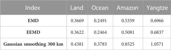
TABLE 2. The RMSEs (unit: cm) of EEMD, EMD and 300 km Gaussian smoothing together with DDK7 in terms of mean mass change.

5 Conclusion

In this paper, EEMD approach is first applied to filter the time-varying gravity field models, together with the EMD approach. We evaluate the filtering efficiency of EEMD in both spectral and spatial scale, respectively. For the real GRACE SH coefficients analysis, the fitting errors of all SH coefficients by EEMD approach are smaller than those of EMD approach. The mean RMS_ratios of all available months for EEMD is 3.45, higher than 3.40 of EMD approach. The results show that EEMD can better filter the noise and extract more geophysical signals. Besides, the simulation results show that all the mean RMSEs of EEMD are smaller than EMD for global, ocean, land, Amazon and Yangtze, indicating that EEMD can extract the closer geophysical signals than EMD with respect to the true signals from CSR mascon data. In summary, we can believe that EEMD is a good choice for extracting the geophysical signals and filtering the noise from GRACE time-varying gravity field models.

Data availability statement

The original contributions presented in the study are included in the article/Supplementary Material, further inquiries can be directed to the corresponding author.

Author contributions

CH performed the data processing, analyzed the experimental results, and drafted the manuscript. FW designed the study, conducted the analysis of the results and revised the manuscript. SZ and XQ checked the performance of this method and revised the manuscript. All authors read and approved the final manuscript.

Funding

This work is mainly funded by the Natural Science Foundation of China (42064001).

Acknowledgments

We appreciate the constructive comments from the editor and two reviewers, which led to significant improvement of the manuscript.

Conflict of interest

The authors declare that the research was conducted in the absence of any commercial or financial relationships that could be construed as a potential conflict of interest.

Publisher’s note

All claims expressed in this article are solely those of the authors and do not necessarily represent those of their affiliated organizations, or those of the publisher, the editors and the reviewers. Any product that may be evaluated in this article, or claim that may be made by its manufacturer, is not guaranteed or endorsed by the publisher.

References

Ai, S., and Xiao, Y. (2022). Empirical mode decomposition filter for temporal gravity field denoising study. Henan Sci. 01, 78–85. (in Chinese).

Google Scholar

Bettadpur, S. (2012). Insights into the Earth System mass variability from CSR-RL05 GRACE gravity fields 14, 6409. EGU General Assembly Conference Abstracts.

Google Scholar

Chambers, D. P., and Bonin, J. A. (2012). Evaluation of Release-05 GRACE time-variable gravity coefficients over the ocean. Ocean Sci. 8 (5), 859–868. doi:10.5194/os-8-859-2012

CrossRef Full Text | Google Scholar

Chen, J., Wilson, C., and Seo, K. W. (2006). Optimized smoothing of Gravity Recovery and Climate Experiment (GRACE) time-variable gravity observations. J. Geophys. Res. Solid Earth 111 (B6). doi:10.1029/2005jb004064

CrossRef Full Text | Google Scholar

Chen, J., Wilson, C., Tapley, B., and Grand, S. (2007). GRACE detects coseismic and post-seismic deformation from the Sumatra-Andaman earthquake. Geophys. Res. Lett. 34 (13). doi:10.1029/2007gl030356

CrossRef Full Text | Google Scholar

Crowley, John W., and Huang, J. (2020). A least-squares method for estimating the correlated error of GRACE models. Geophys. J. Int. 221 (3), 1736–1749. doi:10.1093/gji/ggaa104

CrossRef Full Text | Google Scholar

Dahle, C., Flechtner, F., Gruber, C., K¨onig, D., K¨onig, R., Michalak, G., et al. (2013). GFZGRACE level-2 processing standards document for level-2 product release 05. Potsdam, Germany: GeoForschungsZen-trum.

Google Scholar

Duan, X. J., Guo, J. Y., Shum, C. K., and Van Der Wal, W. (2009). On the postprocessing removal of correlated errors in GRACE temporal gravity field solutions. J. Geodesy 83 (11), 1095–1106. doi:10.1007/s00190-009-0327-0

CrossRef Full Text | Google Scholar

Feng, W. (2013). Research on satellite gravity monitoring of regional land water and sea level changes. Beijing, China: University of Chinese Academy of Sciences. (in Chinese).

Google Scholar

Guo, F., Sun, Z., and Wang, F. (2018). Research progress of filtering approach for time-varying gravity field of GRACE satellite. Prog. Geophys. 33 (5), 1783–1788. (in Chinese).

Google Scholar

Guo, W., Huang, L., Chen, C., Zou, H., and Liu, Z. (2016). Elimination of end effects in local mean decomposition using spectral coherence and applications for rotating machinery. Digit. signal Process. 55, 52–63. doi:10.1016/j.dsp.2016.04.007

CrossRef Full Text | Google Scholar

Huan, C., Wang, F., and Zhou, S. (2022). Empirical mode decomposition for post-processing the GRACE monthly gravity field models. Acta Geodyn. Geomaterialia 19 (4), 281–290. doi:10.13168/agg.2022.0013

CrossRef Full Text | Google Scholar

Huang, N. E., Shen, Z., Long, S. R., Wu, M. C., Shih, H. H., Zheng, Q., et al. (1998). The empirical mode decomposition and the Hilbert spectrum for nonlinear and non-stationary time series analysis. Proc. R. Soc. Lond. Ser. A Math. Phys. Eng. Sci. 454, 903–995. doi:10.1098/rspa.1998.0193

CrossRef Full Text | Google Scholar

Kusche, J. (2007). Approximate decorrelation and non-isotropic smoothing of time-variable GRACE-type gravity field models. J. Geodesy 81 (11), 733–749. doi:10.1007/s00190-007-0143-3

CrossRef Full Text | Google Scholar

Kusche, J., Schmidt, R., Petrovic, S., and Rietbroek, R. (2009). Decorrelated GRACE time-variable gravity solutions by GFZ, and their validation using a hydrological model. J. Geodesy 83 (10), 903–913. doi:10.1007/s00190-009-0308-3

CrossRef Full Text | Google Scholar

Landerer, F. W., Dickey, J. O., and Güntner., A. (2010). Terrestrial water budget of the Eurasian pan-arctic from GRACE satellite measurements during 2003–2009. J. Geophys. Res. Atmos. 115 (D23), D23115. doi:10.1029/2010jd014584

CrossRef Full Text | Google Scholar

Lei, Y., He, Z., and Zi, Y. (2009). Application of the EEMD method to rotor fault diagnosis of rotating machinery. Mech. Syst. Signal Process. 23 (4), 1327–1338. doi:10.1016/j.ymssp.2008.11.005

CrossRef Full Text | Google Scholar

Lu, F., You, W., and Fan, D. (2015). Water storage and seawater quality in Mainland China in recent 10 years retrieved from GRACE RL05 data. Acta Geod. Cartogr. Sinica 44 (2), 160.

Google Scholar

Mejia-Barron, A., Valtierra-Rodriguez, M., Granados-Lieberman, D., Olivares-Galvan, J. C., and Escarela-Perez, R. (2017). The application of EMD-based methods for diagnosis of winding faults in a transformer using transient and steady state currents. Measurement 117, 371–379. doi:10.1016/j.measurement.2017.12.003

CrossRef Full Text | Google Scholar

Ning, J., Wang, Z., and Chao, N. (2016). Research status and progress of the international next-generation satellite gravity detection program. J. Wuhan Univ. Inf. Sci. Ed. 41 (1), 1–8. (in Chinese).

Google Scholar

Niu, Y., and Xiong, C. (2018). Analysis of the dynamic characteristics of a suspension bridge based on RTK-GNSS measurement combining EEMD and a wavelet packet technique. Meas. Sci. Technol. 29 (8), 085103. doi:10.1088/1361-6501/aacb47

CrossRef Full Text | Google Scholar

Prevost, P., Chanard, K., Fleitout, L., Calais, E., Walwer, D., van Dam, T., et al. (2019). Data-adaptive spatio-temporal filtering of GRACE data. Geophys. J. Int. 219 (3), 2034–2055. doi:10.1093/gji/ggz409

CrossRef Full Text | Google Scholar

Sasgen, I., Martinec, Z., and Fleming, K. (2007). Wiener optimal combination and evaluation of the Gravity Recovery and Climate Experiment (GRACE) gravity fields over Antarctica. J. Geophys. Res. Solid Earth 112 (B4). doi:10.1029/2006jb004605

CrossRef Full Text | Google Scholar

Schmidt, R., Petrovic, S., Güntner, A., Barthelmes, F., Wünsch, J., and Kusche, J. (2008). Periodic components of water storage changes from GRACE and global hydrology models. J. Geophys. Res. Solid Earth 113 (B8). doi:10.1029/2007jb005363

CrossRef Full Text | Google Scholar

Schrama, E. J. O., Wouters, B., and David, A. (2007). Signal and noise in Gravity Recovery and Climate Experiment (GRACE) observed surface mass variations. J. Geophys. Res. Solid Earth 112 (B8), B08407. doi:10.1029/2006jb004882

CrossRef Full Text | Google Scholar

Shen, Y., Wang, F., and Chen, Q. (2021). Weighted multichannel singular spectrum analysis for postprocessing GRACE monthly gravity field models by considering the formal errors. Geophys. J. Int. 226 (3), 1997–2010. doi:10.1093/gji/ggab199

CrossRef Full Text | Google Scholar

Shu, G., and Liang, X. (2007). Identification of complex diesel engine noise sources based on coherent power spectrum analysis. Mech. Syst. Signal Process. 21 (1), 405–416. doi:10.1016/j.ymssp.2006.06.001

CrossRef Full Text | Google Scholar

Tapley, B., Bettadpur, S., Ries, J., Thompson, P., and Watkins, M. (2004). GRACE measurements of mass variability in the Earth system. Science 305, 503–505. doi:10.1126/science.1099192

PubMed Abstract | CrossRef Full Text | Google Scholar

Velicogna, I., and Wahr, J. (2013). Time-variable gravity observations of ice sheet mass balance: Precision and limitations of the GRACE satellite data. Geophys. Res. Lett. 40 (12), 3055–3063. doi:10.1002/grl.50527

CrossRef Full Text | Google Scholar

Vishwakarma, B. D., Devaraju, B., and Sneeuw, N. (2016). Minimizing the effects of filtering on catchment scale GRACE solutions. Water Resour. Res. 52 (8), 5868–5890. doi:10.1002/2016wr018960

CrossRef Full Text | Google Scholar

Wahr, J., Molenaar, M., and Bryan, F. (1998). Time variability of the Earth's gravity field: Hydrological and oceanic effects and their possible detection using GRACE. J. Geophys. Res. Solid Earth 103 (B12), 30205–30229. doi:10.1029/98jb02844

CrossRef Full Text | Google Scholar

Wang, F., Shen, Y., Chen, T., Chen, Q., and Li, W. (2020). Improved multichannel singular spectrum analysis for post-processing GRACE monthly gravity field models. Geophys. J. Int. 223 (2), 825–839. doi:10.1093/gji/ggaa339

CrossRef Full Text | Google Scholar

Wang, L., Davis, J. L., Hill, E. M., and Tamisiea, M. E. (2016). Stochastic filtering for determining gravity variations for decade-long time series of GRACE gravity. J. Geophys. Res. Solid Earth 121 (4), 2915–2931. doi:10.1002/2015jb012650

CrossRef Full Text | Google Scholar

Watkins, M., and Yuan, D. N.(2012). JPL Level-2 processing standards document for Level-2 product release 05. Report No. GRACE.

Google Scholar

Wouters, B., and Schrama, E. J. (2007). Improved accuracy of GRACE gravity solutions through empirical orthogonal function filtering of spherical harmonics. Geophys. Res. Lett. 34 (23). doi:10.1029/2007gl032098

CrossRef Full Text | Google Scholar

Wu, Z., and Huang, N. E. (2009). Ensemble empirical mode decomposition: A noise-assisted data analysis method. Adv. Adapt. data analysis 1 (1), 1–41. doi:10.1142/s1793536909000047

CrossRef Full Text | Google Scholar

Yi, S., and Sneeuw, N. (2022). A novel spatial filter to reduce north–south striping noise in GRACE spherical harmonic coefficients. J. Geodesy 96 (4), 23–17. doi:10.1007/s00190-022-01614-z

CrossRef Full Text | Google Scholar

Zhan, J., Wang, Y., and Hao, X. (2011). Improved approach for removal of correlated errors in GRACE data. Acta Geod. Cartogr. Sinica 40 (4), 442–446.

Google Scholar

Zhang, Z., Chao, B., Lu, Y., and Hsu, H. T. (2009). An effective filtering for GRACE time-variable gravity: Fan filter. Geophys. Res. Lett. 36 (17). doi:10.1029/2009gl039459doi:L17311

CrossRef Full Text | Google Scholar