Concurrent estimation of seismic reflectivity and Q by using an optimal dictionary learning method

The seismic reflectivity and quality factor Q play an important role in seismic processing and interpretation, such as improving the resolution of seismic data and enhancing the reservoir identification. Most methods estimate seismic reflectivity and Q separately. However, the error of Q model has a negative impact on the reflectivity estimation and the interference of reflectivity makes Q estimates less reliable. In this paper, we propose a new method for concurrent estimation of seismic reflectivity and Q by using optimal dictionary learning. This new method first constructs a complete dictionary based on the non-stationary convolution model, then computes the reflectivity series under different dictionary matrices with the corresponding referencing Q values, and finally selects the optimal dictionary matrix by comprehensively analyzing the residual and reflectivity sparsity so as to obtain seismic reflectivity and Q simultaneously. The results of synthetic and real data examples test confirm the effectiveness of the proposed method. The proposed method provides accurate estimation of seismic reflectivity and Q, improves the vertical resolution without losing weak events and offers more accurate information concerning stratigraphic features in great details.

1 Introduction

Seismic attenuation is ubiquitous because of the earth anelasticity, and it can lead to amplitude decay and phase distortion of the seismic wavelet (Futterman, 1962). The seismic quality factor Q, an important parameter for characterization of rocks, measures seismic attenuation. Seismic reflectivity and Q are sensitive to the geologic information such as lithology and fluid (Winkler and Nur, 1982). Hence, accurate estimation of seismic reflectivity and Q has an important role in seismic processing and interpretation, such as improving the resolution of seismic data and enhancing the reservoir identification.

Seismic reflectivity is commonly computed by the deconvolution methods based on the stationary convolution model, which assumes that the stationary seismic data as input (Velis, 2008). Therefore, the seismic data should be compensated for the anelastic attenuation effects before using the conventional methods to estimate reflectivity. Margrave (1998) extends the stationary convolution model to a non-stationary one by the constant Q theory (Kjartansson, 1979). And then Margrave et al. (2011) develop a non-stationary deconvolution method that estimates reflectivity using the Gabor transform. This method requires non-stationarity propagating wavelets. Chai et al. (2014) present a non-stationary sparse reflectivity inversion method to estimate reflectivity. The non-stationarity seismic data is addressed by non-stationary deconvolution so as to estimate the seismic reflectivity, but the Q value need to been estimated in advance. The computational accuracy of the seismic reflectivity depends on the estimated Q value.

Many methods have been proposed for Q estimation from seismic data, such as the spectral ratio method (McDonal et al., 1958; Hauge, 1981; Blias, 2012; Reine et al., 2012; Nakata et al., 2020), the matching method (White, 1980), the amplitude decay method (Tonn, 1991), the analytical signal method (Engelhard, 1996), the frequency shift method (Quan and Harris, 1997; Zhang and Ulrych, 2002; Gao and Yang, 2007; Hu et al., 2013; Matsushima et al., 2016; Li et al., 2020; Yang et al., 2020), the Q-tomography method (Brzostowski and McMechan, 1992; Dutta and Schuster, 2016) and the Q-analysis method (Wang, 2004; 2014). Among the above-mentioned methods, the spectral ratio method and the frequency shift method are widely used in practice, which estimate Q values by comparing the frequency content of two individual waveforms at different depths or time levels. These methods suffer from the problem of instability because they are very sensitive to layering effects and random noise.

Most methods estimate seismic reflectivity and Q separately. However, the error of Q model has a negative impact on the reflectivity estimation (Shao et al., 2019), and the interference of reflectivity makes Q estimates less reliable (Hackert and Parra, 2004; Xue et al., 2020). Gholami (2015) proposes a semi-blind non-stationary deconvolution method to determine both the reflectivity and Q models simultaneously. And then Aghamiry and Gholami (2018) develop this method for interval Q estimation based on the adaptive parametric dictionary learning. This method only uses the sparsity of the earth impulse response to determine the Q model.

In this paper, we propose a new method to estimate the seismic reflectivity and Q concurrently by using optimal dictionary learning. First, we review the basic theory of the non-stationary convolution and introduce our new method. Then, we test the new method for seismic reflectivity and Q estimation by the synthetic examples using simulated data. Finally, we apply and validate the new method on real seismic data. The synthetic and real data examples are presented confirming high performance of the new method.

2 Theory and methodology

2.1 Theory of non-stationary convolution

The traditional convolution model of a seismic trace is often stated as (Robinson, 1967)

$y_{stat}\left(t\right)=w\left(t\right)*r\left(t\right)+e\left(t\right)=\underset{-\infty }{\overset{\infty }{{\displaystyle \int }}}w\left(t-\tau \right)r\left(\tau \right)d\tau +e\left(t\right),(1)$

where t and $\tau$ are the time indexes, $y_{stat}\left(t\right)$ is the stationary seismic trace, $w\left(t\right)$ is the seismic wavelet, $r\left(t\right)$ is the seismic reflectivity, and $e\left(t\right)$ is the random noise term. We can write a matrix equivalent expression for Eq. 1, as

$\mathbf{y}=\mathbf{W}\mathbf{r}+\mathbf{e},(2)$

where $\mathbf{W}$ is a Toeplitz matrix formed from seismic wavelet; $\mathbf{y}$, $\mathbf{r}$ and $\mathbf{e}$ are the vector forms of the seismic trace, the seismic reflectivity series and the random noise term respectively.

We first convolute the reflectivity $r\left(t\right)$ and delta function $\delta \left(t\right)$ to derive the mathematical formula of the non-stationary convolution model (Gholami, 2015)

$x\left(t\right)=\underset{-\infty }{\overset{\infty }{{\displaystyle \int }}}\delta \left(t-\tau \right)r\left(\tau \right)d\tau .(3)$

Using $x\left(t\right)$ to replace $r\left(t\right)$ in Eq. 1, we have

$y_{stat}\left(t\right)=w\left(t\right)*x\left(t\right)+e\left(t\right).(4)$

We can write a matrix equivalent expression for Eq. 4, as

$\mathbf{y}=\mathbf{W}\mathbf{x}+\mathbf{e}.(5)$

Considering the attenuation effect of seismic wave, the attenuation coefficient (Aghamiry and Gholami, 2018) is introduced into the delta function to obtain

$\stackrel{\wedge }{\delta }\left(f,\tau \right)=\alpha \left(f,\tau \right)\stackrel{\wedge }{\delta }\left(f,\tau -1\right)={\displaystyle \prod }_{k=1}^{\tau }\alpha \left(f,k\right)\stackrel{\wedge }{\delta }\left(f,0\right),(6)$

where $f$ is the frequency index, $\stackrel{\wedge }{\delta }\left(f,\tau \right)$ is the frequency spectrum of the delta function, $\stackrel{\wedge }{\delta }\left(f,\tau \right)={\mathcal{F}}_{t\to f}\left\{\delta \left(t,\tau \right)\right\}$, and ${\mathcal{F}}_{t\to f}$ denotes the Fourier transform with respect to t. $\stackrel{\wedge }{\delta }\left(f,0\right)$ is the frequency spectrum of the delta function at the initial time. Using the constant Q theory (Aki and Richards, 1980), the attenuation coefficient can be defined as follows (Aki and Richards, 1980; Gholami, 2015):

$\alpha \left(f,\tau \right)=\exp \left(-\frac{\pi \beta \left(f\right)}{Q\left(\tau \right)}-\frac{i2\pi f}{N}\right),(7)$

where $\alpha \left(f,\tau \right)$ is the attenuation coefficient on the propagation time $\tau$, $\beta \left(f\right)$ is a function of frequency and its role is to impose some physical constraints, $N$ is the number of data samples, and $Q\left(\tau \right)$ is the seismic quality factor which is a function changing with the propagation time. The average quality factor can be defined as follows (Margrave et al., 2011):

$\frac{t}{Q_{ave}\left(t\right)}={\displaystyle \sum }_{k=1}^K\frac{\Delta t_k}{Q_k},(8)$

where $Q_{ave}\left(t\right)$ is the average of the seismic quality factor as a function of the propagation time, k = 1, … , K, K is the total number of assumed Q layers, $\Delta t_k$ and $Q_k$ are the traveltime and Q value through the kth layer, respectively.

In Eq. 7, $\beta \left(f\right)=\left|f\right|-i\mathcal{H}\left|f\right|$, where $\mathcal{H}$ is the Hilbert transform operator. We can rewrite Eq. 7 into the following matrix form (Aghamiry and Gholami, 2018)

$\widehat{\mathbf{\Delta }}=\left[\begin{array}{cccc}\alpha {\left(f,\tau \right)}^0& \alpha {\left(f,\tau \right)}^1& ...& \alpha {\left(f,\tau \right)}^{N-1}\end{array}\right],(9)$

where $\mathbf{\Delta }$ is the attenuation operator in the time domain and $\widehat{\mathbf{\Delta }}$ is the frequency domain representation of it. Figure 1A shows the attenuation matrix $\mathbf{\Delta }$ for a constant Q = 30, and Figure 1B shows some columns of this matrix. This figure suggests that the shape of the propagated delta functions is severely affected by the attenuation effect. According to Eqs 3, 9, we have

$\mathbf{x}={\mathbf{F}}^{-1}\widehat{\mathbf{\Delta }}\mathbf{r}=\mathbf{\Delta }\mathbf{r},(10)$

where ${\mathbf{F}}^{-1}$ is the inverse Fourier transform matrix. Substitute Eq. 10 into Eq. 5 and obtain the matrix form of the non-stationary convolution model

$\mathbf{y}=\mathbf{W}\mathbf{\Delta }\mathbf{r}+\mathbf{e}.(11)$

FIGURE 1

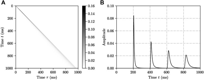
FIGURE 1. (A) Attenuation matrix $\Delta$ (Q = 30) and (B) some of its columns.

2.2 Estimation of seismic reflectivity and Q

We construct a dictionary matrix corresponding to the Q model. Let

$\mathbf{G}=\mathbf{W}\mathbf{\Delta }.(12)$

Substitute Eq. 12 into Eq. 11 and obtain

$\mathbf{y}=\mathbf{G}\mathbf{r}+\mathbf{e}.(13)$

The dictionary matrix $\mathbf{G}$ is related to Q value. The sparsity of the seismic reflectivity series can be used to determine the corresponding dictionary matrix $\mathbf{G}$ in the optimal case (Aghamiry and Gholami, 2018), so as to obtain the quality factor. We first assume that $\mathbf{G}$ is known, then the solution to the seismic reflectivity series $\mathbf{r}$ can be converted to an optimization problem, which is expressed in the following form (Gholami, 2015; Aghamiry and Gholami, 2018)

$\mathrm{a}\mathrm{r}\mathrm{g}\mathrm{m}\mathrm{i}\mathrm{n}{‖\mathbf{r}‖}_1\mathrm{s}\mathrm{u}\mathrm{b}\mathrm{j}\mathrm{e}\mathrm{c}\mathrm{t}\mathrm{t}\mathrm{o}{‖\mathbf{y}\mathbf{-}\mathbf{G}\mathbf{r}‖}_2^2\le \xi ,(14)$

or

$\mathrm{a}\mathrm{r}\mathrm{g}\mathrm{m}\mathrm{i}\mathrm{n}\left\{{‖\mathbf{y}\mathbf{-}\mathbf{G}\mathbf{r}‖}_2^2+\lambda {‖\mathbf{r}‖}_1\right\},(15)$

where $\xi$ is an error bound of the data, $\lambda$ is the regularization parameter and ${‖‖}_p$ denotes the p-norm. Due to the sparseness of the reflectivity series, it is necessary to use the sparse norm as much as possible to constrain it. The value of the p-norm in [0, 1] can ensure its sparsity. The value of the reflectivity series always lies between −1 and 1, so we use p=1/2 to measure the sparsity of the reflectivity in this paper.

In the inverse Q filtering method, the first step is usually to estimate the Q value, and then use the estimated Q value to perform inverse Q filtering, so the inverse Q filtering result depends on the estimated Q value. In this paper, we adopt a similar matching pursuit algorithm in dictionary learning to solve Eq. 14. The traditional matching pursuit algorithm needs to construct the dictionary matrices in Hilbert space, and each column of the dictionary matrices is dealed with normalization. In this paper, however, we construct a complete dictionary based on the theory of the non-stationary convolution model, and compute the reflectivity series under different dictionary matrices with the corresponding referencing Q values. Finally, we select the optimal dictionary matrix by comprehensively analyzing the residual and reflectivity sparsity, so as to obtain the seismic reflectivity and Q concurrently. The complete dictionary can describe changes in seismic amplitude over time, which is more in line with the laws of physics.

In the specific implementation process, the first step is to construct a three-dimensional dictionary matrix ${\mathbf{G}}_{dic}$ as shown in Figure 2. The first dimension of this matrix is related to the value of the quality factor. Slicing along the first dimension is a two-dimensional N×N matrix $\mathbf{G}$, with the N th column representing the seismic wave at the propagation time N ms under the quality factor corresponding to the slice. According to the theory of the average Q value, we construct the dictionary matrix $\mathbf{G}$ by extracting the corresponding column from the matrix ${\mathbf{G}}_{dic}$ for the multi-layered signal (multi-segment Q value), which avoids the reduplicate calculation for constructing the matrices in every loop and significantly improves the computational efficiency. The second step is to initialize the reference Q values. The exact approach is to select a certain number of Q values in a reasonable range in logarithm scale as the reference Q values. The third step is to perform the subsection process for the seismic signals. The seismic signal is divided to several segments according to the rough seismic horizon to estimate the reflectivity and Q. For each seismic signal segment, the similar matching pursuit algorithm is used to compute the reflectivity series under the different referencing Q values, so as to obtain the corresponding residual $\mathbf{\epsilon }={‖\mathbf{y}-\mathbf{G}\mathbf{r}‖}_2^2$ and the sparsity of the seismic reflectivity series $\mathbf{\sigma }={‖\mathbf{r}‖}_{1/2}$. ${\mathbf{\epsilon }}^{*}$ and ${\mathbf{\sigma }}^{*}$ are defined to represent the normalization of $\mathbf{\epsilon }$ and $\mathbf{\sigma }$ respectively, and we can construct the following formula to evaluate the estimation results

$\mathbf{\xi }=\left(1-\varphi \right){\mathbf{\epsilon }}^{*}+\varphi {\mathbf{\sigma }}^{*},(16)$

where $\mathbf{\xi }$ is a synthetic criterion, and $\varphi$ is an adjustable constant, measuring the weight of sparsity versus residual when evaluates the estimation results. A pseudo-code for this procedure is presented in Algorithm 1.

FIGURE 2

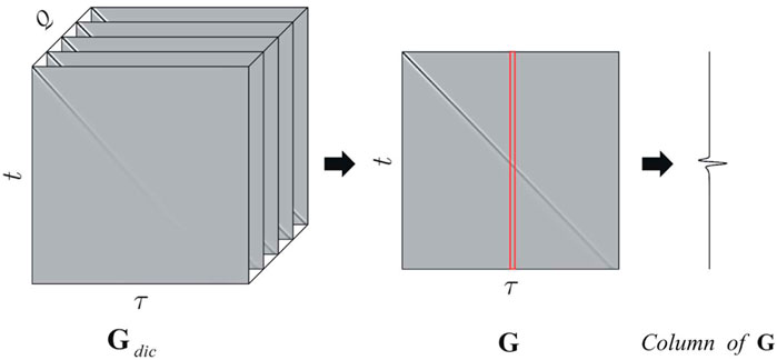
FIGURE 2. The structure of the dictionary matrix.

Algorithm 1. A pseudo-code for seismic reflectivity and Q estimation.

1 Input: $\mathbf{y}$, the number of signal segment $n_s$, the number of the reference Q $n_q$

2 Initialize: $\mathbf{W}$, ${\mathbf{G}}_{dic}$, the reference Q values

3 for $i=1,...,n_s$:

4 for $j=1,...,n_q$:

5 ${\mathit{q}}_{\mathit{i}}\leftarrow Q_j$

6 calculate ${\mathbf{q}}_{ave}$ via $\mathbf{q}$

7 according to ${\mathbf{q}}_{ave}$, construct the dictionary matrix ${\mathbf{G}}_{\mathit{j}}$ by extracting the corresponding columns from ${\mathbf{G}}_{dic}$

8 ${\mathbf{r}}_{\mathit{j}}^{\prime }=\mathrm{a}\mathrm{r}\mathrm{g}\mathrm{m}\mathrm{i}\mathrm{n}\left\{{‖\mathbf{y}-{\mathbf{G}}_{\mathit{j}}{\mathbf{r}}_{\mathit{j}}^{\prime }‖}_2^2+\lambda {‖{\mathbf{r}}_{\mathit{j}}^{\prime }‖}_{1/2}\right\}$

9 ${\mathbf{\epsilon }}_{\mathit{j}}={‖\mathbf{y}-{\mathbf{G}}_{\mathit{j}}{\mathbf{r}}_{\mathit{j}}^{\prime }‖}_2^2$

10 ${\mathbf{\sigma }}_{\mathit{j}}={‖{\mathbf{r}}_{\mathit{j}}^{\prime }‖}_{1/2}$

11 end

12 $\mathbf{\xi }=\left(1-\varphi \right){\mathbf{\epsilon }}^{*}+\varphi {\mathbf{\sigma }}^{*}$

13 find the index of the minimum value for $\mathbf{\xi }$

14 ${\mathbf{r}}_{\mathit{i}}\leftarrow {\mathbf{r}}_{index}^{\prime }$, ${\mathbf{q}}_{\mathit{i}}\leftarrow Q_{index}$

15 end

16 Output: $\mathbf{r}$, $\mathbf{q}$

3 Synthetic examples

In this section, we test the new method for seismic reflectivity and Q estimation of synthetic data. Both the constant-Q and the interval-Q models are designed for this purpose.

3.1 Seismic reflectivity and Q estimation of the constant-Q model

We first test the performance of the new method for seismic reflectivity and Q estimation of the constant-Q model. Some synthetic traces have been generated by convolving the reflectivity with a Ricker wavelet of dominant frequency 35 Hz and then contaminated by the random noises. The recording time is 1 s with the sample interval at 1 ms. These wavelet and recording parameters are used for all the synthetic examples in this paper.

Figures 3A–C shows the simple synthetic traces attenuated by using the constant-Q model with different Q values (Q = 30, Q = 60 and Q = 110) and contaminated by the 0.1% random noises. Here, the reflectivity series of 0.5, −0.6 and 0.7 are set at 250, 500, and 750 ms respectively, and no interference occurred between the reflections. The new method is applied to these simple traces for the reflectivity and constant Q estimation. Thirty logarithmically spaced Q values in the range [10, 120] are selected to run Algorithm 1. The estimated reflectivity series are shown in Figures 3D–F. As seen from these figures, the estimated reflectivity series are very close to the true values. The corresponding estimations of the Q values are showed in Figures 3G–I, showing a relatively good match with the true Q values, as shown in these figures by the red lines for comparison.

FIGURE 3

FIGURE 3. Simple synthetic traces attenuated by using constant-Q model with different Q values: (A) Q = 30, (B) Q = 60, and (C) Q = 110. The estimated reflectivity series are shown in (D–F). The true non-zero reflectivity coefficients are shown by the red points. The corresponding estimations of the Q values are showed in (G–I). The true Q values are shown in red lines.

Figures 4A–C shows the complex synthetic traces attenuated by using the constant-Q model (Q = 60) and contaminated by random noises of different levels (0.1%, 5% and 10%). Here, the high reflections are set at 333, 500, and 666 ms, and the corresponding reflection coefficients are 0.75, −0.75 and 0.75, respectively. At other times, the reflection coefficients are set randomly. There are some reflection interferences from the adjacent reflections in the complex synthetic traces. These complex traces are used to test the new method for the reflectivity and constant-Q estimation. Thirty logarithmically spaced Q values in the range [10, 120] are also selected to run Algorithm 1. The estimated reflectivity series are shown in Figures 4D–F. As seen from these results, the new method improves the resolution and gives satisfactory results in the case of complex waves. The corresponding estimations of the Q values are showed in Figures 4G–I, which show good consistency with the true Q values.

FIGURE 4

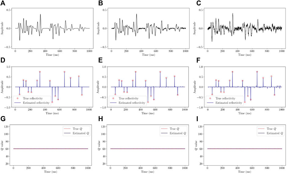
FIGURE 4. Complex synthetic traces attenuated by using constant-Q model (Q = 60) and contaminated by random noises of different levels: (A) 0.1%, (B) 5%, and (C) 10%. The estimated reflectivity series are shown in (D–F). The true non-zero reflectivity coefficients are shown by the red points. The corresponding estimations of the Q values are showed in (G–I). The true Q values are shown in red lines.

3.2 Seismic reflectivity and Q estimation of the interval-Q model

We next test the performance of the new method for seismic reflectivity and Q estimation of the interval-Q model. Similar to the previous examples, some synthetic traces have been generated by convolving the reflectivity with a Ricker wavelet of dominant frequency 35 Hz, and then different random noises have been added to the resulting traces. The new method is applied to these synthetic traces for the reflectivity and interval-Q estimation. Algorithm 1 is performed for thirty logarithmically spaced Q values in the range [10, 120].

Figures 5A–C shows the simple synthetic traces attenuated by using the different interval-Q models and contaminated by the 0.1% random noises. Here, the reflectivity series of 0.3, 0.4, −0.6, 0.7, −0.6, 0.4 and 0.3 are set at 111, 222, 333, 500, 666, 777, and 888 ms respectively, and no interference occurred between the reflections. The estimated reflectivity series are shown in Figures 5D–F. The corresponding estimations of the Q values are showed in Figures 5G–I.

FIGURE 5

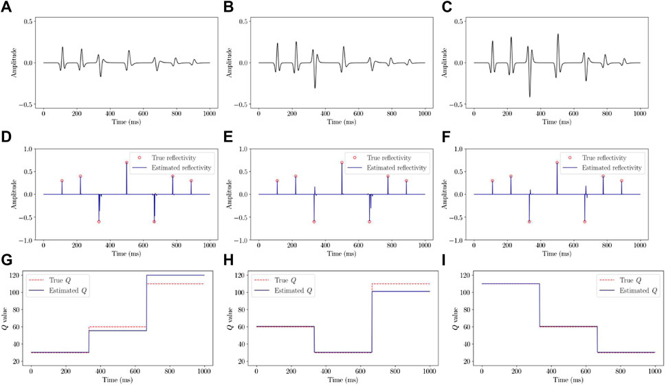
FIGURE 5. Simple synthetic traces attenuated by using interval-Q model with different Q values: (A) Q = (30, 60, 110), (B) Q = (60, 30, 110), and (C) Q = (110, 60, 30). The estimated reflectivity series are shown in (D–F). The true non-zero reflectivity coefficients are shown by the red points. The corresponding estimations of the Q values are showed in (G–I). The true Q values are shown in red lines.

Figures 6A–C shows the complex synthetic traces attenuated by using the interval-Q model (Q = 60, 30, 110) and each contaminated by random noises of different levels (0.1%, 5% and 10%). Here, the high reflections are set at 333, 500, and 666 ms, and the corresponding reflection coefficients are 0.7, −0.7 and 0.7, respectively. At other times, the reflection coefficients are set randomly. The complex synthetic traces contain some reflection interferences from the adjacent reflections. The final obtained reflectivity series are shown in Figures 6D–F. The corresponding estimations of the Q values are showed in Figures 6G–I.

FIGURE 6

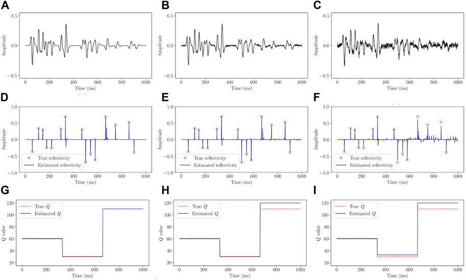
FIGURE 6. Complex synthetic traces attenuated by using interval-Q model (Q = 60, 30, 110) and contaminated by random noises of different levels: (A) 0.1%, (B) 5%, and (C) 10%. The estimated reflectivity series are shown in (D–F). The true non-zero reflectivity coefficients are shown by the red points. The corresponding estimations of the Q values are showed in (G–I). The true Q values are shown in red lines.

As seen from these results, the estimations of the reflectivity series are very accurate and the estimated Q values are relatively close to the true values in all the cases. Furthermore, the accuracy of the estimates is related to the noise level, which decreases as the noise level increases under normal circumstances. The new method improves the resolution by removing the wavelet and attenuation effects even in the case of high-level noises, especially at places with great attenuation effects.

For comparison, we also perform the Gabor deconvolution (Margrave et al., 2011) for the reflectivity estimation corresponding to the synthetic traces shown in Figures 6A–C. The Gabor deconvolution estimates and corrects for the effects of source wavelet and anelastic attenuation (Margrave et al., 2011). The corresponding estimated reflectivity series are shown in Figure 7. It is clearly seen from Figures 6, 7 that the accuracy of the reflectivity estimation by the Gabor deconvolution is not better than that by our proposed method.

FIGURE 7

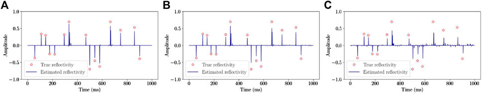
FIGURE 7. The estimated reflectivity series by the Gabor deconvolution. (A) The estimated reflectivity series corresponding to the synthetic traces shown in Figure 6A. (B) The estimated reflectivity series corresponding to the synthetic traces shown in Figure 6B. (C) The estimated reflectivity series corresponding to the synthetic traces shown in Figure 6C. The true non-zero reflectivity coefficients are shown by the red points.

In addition, we compare the proposed method with the conventional spectral ratio method (Hauge, 1981) for the Q estimation. The results of the Q estimation are reported in Table 1. It can be seen from Table 1 that the proposed method provides more accurate Q values than the spectral ratio method in all cases. The new method uses both the amplitude and phase information of the attenuation operator, and regularizes the estimated Q by the sparsity information of the seismic reflectivity series. However, the conventional spectral ratio method only uses the amplitude information to determine the Q value, and the spectral interference from the adjacent reflections limits it (Xue et al., 2020). Hence, the Q values estimated by the new method are more accurate than the results provided by the conventional spectral ratio method.

TABLE 1

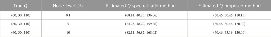
TABLE 1. The results of the Q estimation by different methods, corresponding to the synthetic traces shown in Figures 6A–C.

4 Real data examples

Finally, we test the performance of the new method with two sets of real stacked seismic data shown in Figures 8A, 9A. The geometric spreading correction and the simple de-noising process have been operated for the real data. The real data represent the 2D poststack sections with the high signal-to-noise ratio and look clean. The seismic wavelet can be extracted from the early part of the data using the blind deconvolution method (Gholami and Sacchi, 2013). In general, the signal can be segmented according to the rough horizon in the seismic data. For computational purposes, the numbers of Q-layers 9 and 5 are assumed for the two sets of real stacked seismic data respectively. For each data set, thirty Q values in the range [20, 400] in logarithm scale are selected to run Algorithm 1. The resulting reflectivity sections are depicted in Figures 8B, 9B, which show the vertical resolution has been greatly improved by the new method, and provide the structural and stratigraphic features in great details. The vertical resolution achieved by the new method is significant and it may have important effects in seismic reservoir characterization of thin layers. The estimated Q models by the proposed method are shown in Figures 8C, 9C. The estimated Q models by the conventional spectral ratio method are shown in Figures 8E, 9E. We perform the inverse Q filtering (Wang, 2006) of the data using the generated Q models. The resulting seismic sections after inverse Q filtering using the estimated Q model by the proposed method are shown in Figures 8D, 9D. The resulting seismic sections after inverse Q filtering using the estimated Q model by the conventional spectral ratio method are shown in Figures 8F, 9F. These resulting seismic sections clearly show improvements in the vertical resolution and more details on stratigraphic features compared to the raw data. Furthermore, it can be seen from these figures that the improved resolution using the estimated Q model by the proposed method is better than the one by the conventional spectral ratio method.

FIGURE 8

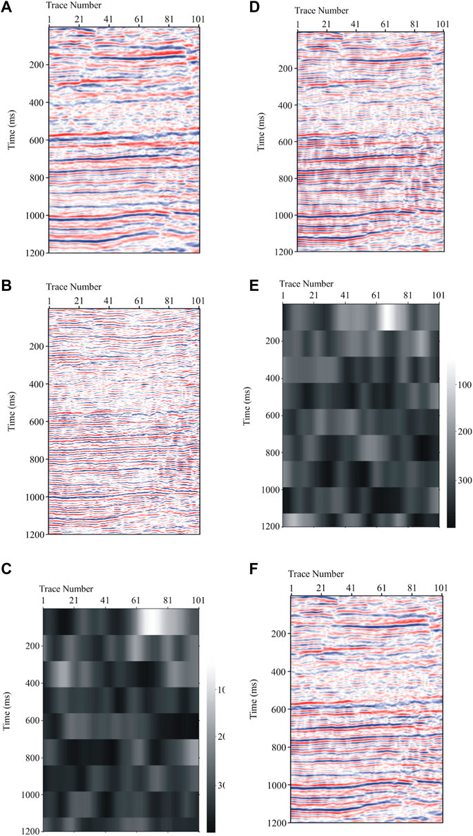
FIGURE 8. (A) A stacked seismic data set, (B) estimated reflectivity section by the proposed method, (C) estimated Q model by the proposed method, (D) seismic section after inverse Q filtering using the estimated Q model by the proposed method, (E) estimated Q model by the conventional spectral ratio method, and (F) seismic section after inverse Q filtering using the estimated Q model by the conventional spectral ratio method.

FIGURE 9

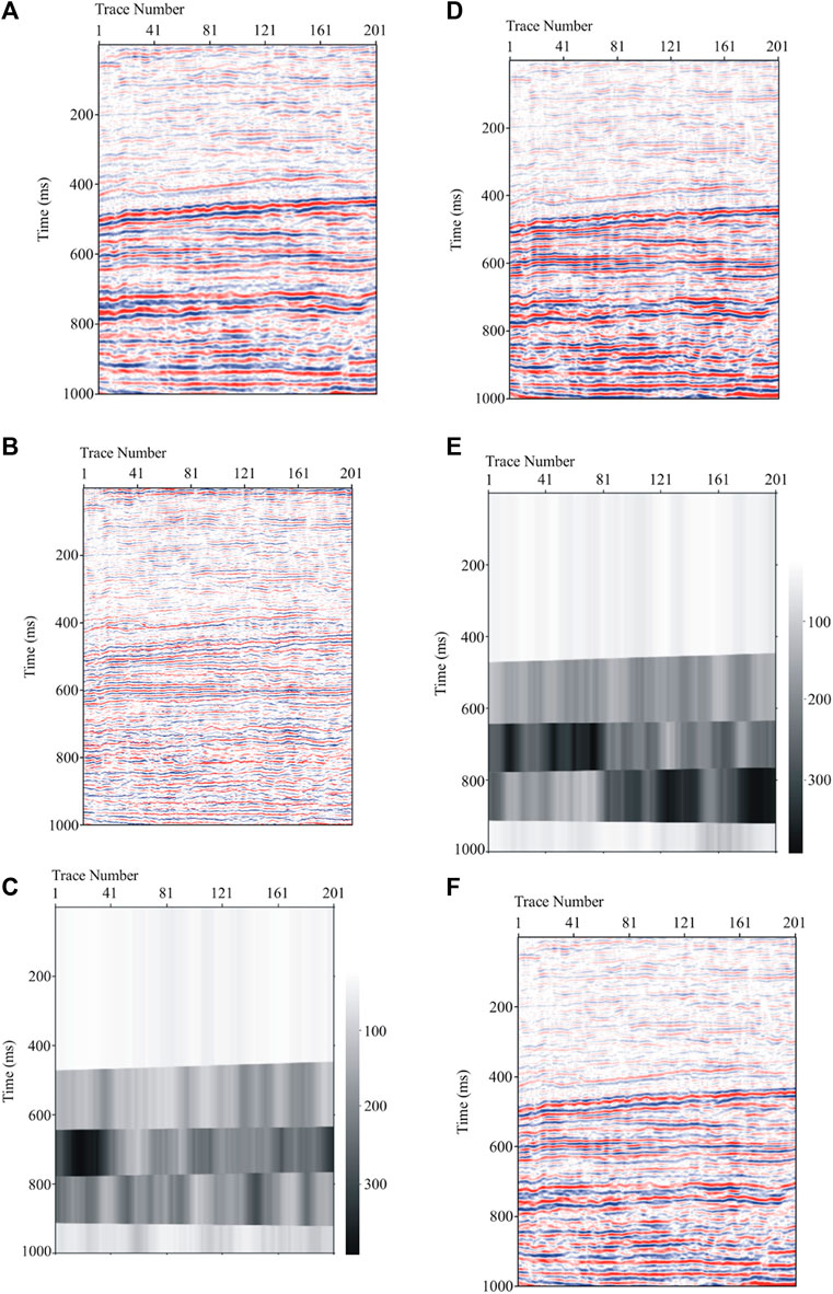
FIGURE 9. (A) A stacked seismic data set, (B) estimated reflectivity section by the proposed method, (C) estimated Q model by the proposed method, (D) seismic section after inverse Q filtering using the estimated Q model by the proposed method, (E) estimated Q model by the conventional spectral ratio method, and (F) seismic section after inverse Q filtering using the estimated Q model by the conventional spectral ratio method.

5 Discussion

In general, the performance of Q estimation methods from seismic data decreases with increasing wavelet interference and noise level (Tu and Lu, 2010; Aghamiry and Gholami, 2018). Our proposed method uses both the amplitude and phase information of the attenuation mechanism, and regularizes the estimated Q model by the sparsity constraint of the seismic reflectivity, but it is also affected by the high-level noises. The accuracy of the estimates decreases as the noise level increases. Therefore, the de-noising process is necessary for the real data with low signal-to-noise ratio. In addition, the proposed method is implemented in a trace by trace manner and takes no account of the lateral continuity. The method of the multichannel form may provide better results.

6 Conclusion

In this paper, we have presented a new method for concurrent estimation of seismic reflectivity and Q by using optimal dictionary learning. This new method first constructs a complete dictionary based on the non-stationary convolution model, then computes the reflectivity series under different dictionary matrices with the corresponding referencing Q values, and finally selects the optimal dictionary matrix by comprehensively analyzing the residual and reflectivity sparsity so as to obtain seismic reflectivity and Q concurrently. Synthetic examples using simulated data demonstrate that the proposed method provides accurate estimation of seismic reflectivity and Q, and improves the resolution by removing the wavelet and attenuation effects. Furthermore, the examples of real data also confirm the effectiveness of the proposed method, which improves the vertical resolution without losing weak events and provides more accurate information concerning stratigraphic features in great details. Thus, the presented method is very useful to improve the vertical resolution and enhance the reservoir identification in seismic processing and interpretation.

Data availability statement

The original contributions presented in the study are included in the article/supplementary material, further inquiries can be directed to the corresponding author.

Author contributions

HYa and HYu studied the method and processed the data. HYa and TX performed the data analysis. HYa wrote and revised the manuscript.

Funding

This work was supported by the National Natural Science Foundation of China (Grant Nos. 92055213 and 41874160), by the Youth Innovation Promotion Association of CAS (2018093), and by the Key Research Program of the Institute of Geology and Geophysics, CAS (Grant No. IGGCAS-201903).

Conflict of interest

The authors declare that the research was conducted in the absence of any commercial or financial relationships that could be construed as a potential conflict of interest.

Publisher’s note

All claims expressed in this article are solely those of the authors and do not necessarily represent those of their affiliated organizations, or those of the publisher, the editors and the reviewers. Any product that may be evaluated in this article, or claim that may be made by its manufacturer, is not guaranteed or endorsed by the publisher.

References

Aghamiry, H. S., and Gholami, A. (2018). Interval-Q estimation and compensation: An adaptive dictionary-learning approach. Geophysics 83 (4), V233–V242. doi:10.1190/geo2017-0001.1

CrossRef Full Text | Google Scholar

Aki, K., and Richards, P. G. (1980). Quantitative seismology: Theory and methods. New York: University Science Books.

Google Scholar

Blias, E. (2012). Accurate interval Q-factor estimation from VSP data. Geophysics 77 (3), WA149–WA156. doi:10.1190/geo2011-0270.1

CrossRef Full Text | Google Scholar

Brzostowski, M., and McMechan, G. (1992). 3D tomographic imaging of near-surface seismic velocity and attenuation. Geophysics 57 (3), 396–403. doi:10.1190/1.1443254

CrossRef Full Text | Google Scholar

Chai, X., Wang, S., Yuan, S., Zhao, J., Sun, L., and Wei, X. (2014). Sparse reflectivity inversion for nonstationary seismic data. Geophysics 79 (3), V93–V105. doi:10.1190/geo2013-0313.1

CrossRef Full Text | Google Scholar

Dutta, G., and Schuster, G. T. (2016). Wave-equation Q tomography. Geophysics 81 (6), R471–R484. doi:10.1190/geo2016-0081.1

CrossRef Full Text | Google Scholar

Engelhard, L. (1996). Determination of seismic-wave attenuation by complex trace analysis. Geophys. J. Int. 125 (2), 608–622. doi:10.1111/j.1365-246X.1996.tb00023.x

CrossRef Full Text | Google Scholar

Futterman, W. I. (1962). Dispersive body waves. J. Geophys. Res. 67 (13), 5279–5291. doi:10.1029/JZ067i013p05279

CrossRef Full Text | Google Scholar

Gao, J., and Yang, S. (2007). On the method of quality factors estimation from zero-offset VSP data. Chin. J. Geophys. (in Chinese) 50 (4), 1026–1040. doi:10.1002/cjg2.1120

CrossRef Full Text | Google Scholar

Gholami, A., and Sacchi, M. D. (2013). Fast 3D blind seismic deconvolution via constrained total variation and GCV. SIAM Journal on Imaging Sciences 6 (4), 2350–2369. doi:10.1137/130905009

CrossRef Full Text | Google Scholar

Gholami, A. (2015). Semi-blind nonstationary deconvolution: Joint reflectivity and Q estimation. Journal of Applied Geophysics 117, 32–41. doi:10.1016/j.jappgeo.2015.02.030

CrossRef Full Text | Google Scholar

Hackert, C. L., and Parra, J. O. (2004). Improving Q estimates from seismic reflection data using well-log-based localized spectral correction. Geophysics 69 (6), 1521–1529. doi:10.1190/1.1836825

CrossRef Full Text | Google Scholar

Hauge, P. S. (1981). Measurements of attenuation from vertical seismic profiles. Geophysics 46 (11), 1548–1558. doi:10.1190/1.1441161

CrossRef Full Text | Google Scholar

Hu, C., Tu, N., and Lu, W. (2013). Seismic attenuation estimation using an improved frequency shift method. IEEE Geoscience and Remote Sensing Letters 10, 1026–1030. doi:10.1109/LGRS.2012.2227933

CrossRef Full Text | Google Scholar

Kjartansson, E. (1979). Constant Q-wave propagation and attenuation. Journal of Geophysical Research 84, 4737–4748. doi:10.1029/JB084iB09p04737

CrossRef Full Text | Google Scholar

Li, H., Greenhalgh, S., Chen, S., Liu, X., and Liu, B. (2020). A robust Q estimation scheme for adaptively handling asymmetric wavelet spectrum variations in strongly attenuating media. Geophysics 85 (4), V345–V354. doi:10.1190/geo2019-0442.1

CrossRef Full Text | Google Scholar

Margrave, G. F., Lamoureux, M. P., and Henley, D. C. (2011). Gabor deconvolution: Estimating reflectivity by nonstationary deconvolution of seismic data. Geophysics 76 (3), W15–W30. doi:10.1190/1.3560167

CrossRef Full Text | Google Scholar

Margrave, G. F. (1998). Theory of nonstationary linear filtering in the Fourier domain with application to time-variant filtering. Geophysics 63 (1), 244–259. doi:10.1190/1.1444318

CrossRef Full Text | Google Scholar

Matsushima, J., Ali, M. Y., and Bouchaala, F. (2016). Seismic attenuation estimation from zero-offset VSP data using seismic interferometry. Geophysical Journal International 204 (2), 1288–1307. doi:10.1093/gji/ggv522

CrossRef Full Text | Google Scholar

McDonal, F. J., Angona, F. A., Mills, R. L., Sengbush, R. L., Van Nostrand, R. G., and White, J. E. (1958). Attenuation of shear and compressional waves in Pierre shale. Geophysics 23 (3), 421–439. doi:10.1190/1.1438489

CrossRef Full Text | Google Scholar

Nakata, R., Lumley, D., Hampson, G., Nihei, K., and Nakata, N. (2020). Waveform-based estimation of Q and scattering properties for zero-offset vertical seismic profile data. Geophysics 85 (4), R365–R379. doi:10.1190/geo2019-0369.1

CrossRef Full Text | Google Scholar

Quan, Y., and Harris, J. M. (1997). Seismic attenuation tomography using the frequency shift method. Geophysics 62 (3), 895–905. doi:10.1190/1.1444197

CrossRef Full Text | Google Scholar

Reine, C., Clark, R. A., and van der Baan, M. (2012). Robust prestack Q-determination using surface seismic data — Part 1: Method and synthetic examples. Geophysics 77 (1), R45–R56. doi:10.1190/geo2011-0073.1

CrossRef Full Text | Google Scholar

Robinson, E. A. (1967). Predictive decomposition of time series with application to seismic exploration. Geophysics 32 (3), 418–484. doi:10.1190/1.1439873

CrossRef Full Text | Google Scholar

Shao, J., Wang, Y., and Chang, X. (2019). “Simultaneous inversion of Q and reflectivity using dictionary learning,” in 89th annual international meeting, SEG, expanded abstracts, 595–599. doi:10.1190/segam2019-3216031.1

CrossRef Full Text | Google Scholar

Tonn, R. (1991). The determination of the seismic quality factor Q from VSP data: A comparison of different computational methods. Geophysical Prospecting 39 (1), 1–27. doi:10.1111/j.1365-2478.1991.tb00298.x

CrossRef Full Text | Google Scholar

Tu, N., and Lu, W.-K. (2010). Improve Q estimates with spectrum correction based on seismic wavelet estimation. Applied Geophysics 7 (3), 217–228. doi:10.1007/s11770-010-0252-2

CrossRef Full Text | Google Scholar

Velis, D. R. (2008). Stochastic sparse-spike deconvolution. Geophysics 73 (1), R1–R9. doi:10.1190/1.2790584

CrossRef Full Text | Google Scholar

Wang, Y. (2004). Q analysis on reflection seismic data. Geophysical Research Letters 31 (17), L17606. doi:10.1029/2004GL020572

CrossRef Full Text | Google Scholar

Wang, Y. (2006). Inverse Q-filter for seismic resolution enhancement. Geophysics 71 (3), V51–V60. doi:10.1190/1.2192912

CrossRef Full Text | Google Scholar

Wang, Y. (2014). Stable Q analysis on vertical seismic profiling data. Geophysics 79 (4), D217–D225. doi:10.1190/geo2013-0273.1

CrossRef Full Text | Google Scholar

White, R. (1980). Partial coherence matching of synthetic seismograms with seismic traces. Geophysical Prospecting 28 (3), 333–358. doi:10.1111/j.1365-2478.1980.tb01230.x

CrossRef Full Text | Google Scholar

Winkler, K. W., and Nur, A. (1982). Seismic attenuation: Effects of pore fluids and frictional sliding. Geophysics 47 (1), 1–15. doi:10.1190/1.1441276

CrossRef Full Text | Google Scholar

Xue, Y.-J., Cao, J.-X., Wang, X.-J., and Du, H.-K. (2020). Estimation of seismic quality factor in the time-frequency domain using variational mode decomposition. Geophysics 85 (4), V329–V343. doi:10.1190/geo2019-0404.1

CrossRef Full Text | Google Scholar

Yang, D., Liu, J., Li, J., and Liu, D. (2020). Q-factor estimation using bisection algorithm with power spectrum. Geophysics 85 (3), V233–V248. doi:10.1190/geo2018-0403.1

CrossRef Full Text | Google Scholar

Zhang, C., and Ulrych, T. J. (2002). Estimation of quality factors from CMP records. Geophysics 67 (5), 1542–1547. doi:10.1190/1.1512799

CrossRef Full Text | Google Scholar