
95% of researchers rate our articles as excellent or good
Learn more about the work of our research integrity team to safeguard the quality of each article we publish.
Find out more
ORIGINAL RESEARCH article
Front. Earth Sci. , 30 March 2023
Sec. Geohazards and Georisks
Volume 11 - 2023 | https://doi.org/10.3389/feart.2023.1118160
This article is part of the Research Topic Geo-information for Geohazard and Georisk View all 11 articles
 Jiangfeng Lv1,2
 Shengwu Qin1*
 Junjun Chen1
 Shuangshuang Qiao1Jingyu Yao1Xiaolan Zhao2Rongguo Cao2Jinhang Yin2
The main purpose of this study was to compare two types of watershed units divided by the hydrological analysis method (HWUs) and mean curvature method (CWUs) for debris flow susceptibility mapping (DFSM) in Northeast China. Firstly, a debris flow inventory map consisting of 129 debris flows and 129 non-debris flows was randomly divided into a ratio of 70% and 30% for training and testing. Secondly, 13 influencing factors were selected and the correlations between these factors and the debris flows were determined by frequency ration analysis. Then, two types of watershed units (HWUs and CWUs) were divided and logistic regression (LR), multilayer perceptron (MLP), classification and regression tree (CART) and Bayesian network (BN) were selected as the evaluation models. Finally, the predictive capabilities of the models were verified using the predictive accuracy (ACC), the Kappa coefficient and the area under the receiver operating characteristic curve (AUC). The mean AUC, ACC and Kappa of four models (LR, MLP, CART and BN) in the training stage were 0.977, 0.931, and 0.861, respectively, for the HWUs, while 0.961, 0.905, and 0.810, respectively, for the CWUs; in the testing stage, were 0.904, 0.818, and 0.635, respectively, for the HWUs, while 0.883, 0.800, and 0.601, respectively, for the CWUs, which showed that HWU model has a higher debris flow prediction performance compared with the CWU model. The CWU-based model can reflect the spatial distribution probability of debris flows in the study area overall and can be used as an alternative model.
According to the China Statistical Yearbook (http://www.stats.gov.cn/tjsj/ndsj/), a total of 7,840 geological disasters occurred in China in 2020, resulting in 197 casualties and direct economic losses of 740 million dollars, of which debris flows accounted for 11.46%. Debris flows are among the most frequent and destructive disasters in mountainous areas (Dash et al., 2022; Jiang et al., 2022; Qiu et al., 2022). Debris flow susceptibility mapping (DFSM), representing where debris flows are likely to occur, plays an important role in debris flow management strategies and has been a hot topic in disaster research worldwide (Ilia and Tsangaratos, 2015; Qin et al., 2019; Sun et al., 2021; Yao et al., 2022).
There are many uncertainties in the process of disaster susceptibility mapping, such as selecting appropriate mapping units, determining evaluation models, screening influencing factors, determining the proportion of training and testing data and others (Tien Bui et al., 2015; Cama et al., 2016; Zezere et al., 2017; Chen et al., 2018; Du et al., 2018; Dou et al., 2019; Qiao et al., 2021). Among the above uncertainty factors, selecting appropriate mapping units is the first step to address disasters and environmental factors. The mapping unit is the basic functional spatial element for dividing the study area (Cama et al., 2016). The term refers to a portion of the land surface which contains a set of ground conditions that differ from the adjacent units across definable boundaries (Van Den Eeckhaut et al., 2009). The selection of mapping units affects the methods used to address the uncertainty in the input data, the model fitting, the reliability of disaster susceptibility mapping and the application of disaster susceptibility mapping in disaster prevention and mitigation (Fausto Guzzetti et al., 1999; Cama et al., 2016; Qiao et al., 2021). At present, mapping units mainly include the following classes: grid cell units, slope units, watershed units, topographic units, geohydrological units, political or administrative units, and unique condition units (Van Den Eeckhaut et al., 2009; Chen et al., 2019; Sun et al., 2020).
For DFSM, grid cell units and watershed units are used frequently. Grid cell units are the most popular mapping units with the same cell size, fast processing speed and simple algorithm (Reichenbach et al., 2018). However, the division of grid cells destroys the integrity of debris flows and is almost completely unrelated to geological and topographic information (Dragut and Eisank, 2011; Wang et al., 2017). Moreover, since debris flows are a dynamic process, the DFSM based on grid cell units cannot comprehensively reflect spatial information (Qin et al., 2019). Watershed refers to the river catchment area that is surrounded by the water-parting line; it is the basic unit for the development and activity of debris flows, and it is the object of exploration, research, and prevention of debris flows. Furthermore, the watershed unit includes the formation area, circulation area, and accumulation area of a debris flow (Qin et al., 2019). Compared with grid cell units, watershed units can completely consider the spatial information of a debris flow. Some scholars have carried out DFSM based on watershed units and obtained reliable results. Qin et al. (2019) explored the accuracy and practicability of mapping units for the evaluation of debris flow susceptibility based on grid cell units and watershed units, and the results showed that watershed units were more feasible than grid cell units when considering the effects of geology and geomorphology on the occurrence of debris flows. Qiao et al. (2021) proposed a region-partitioning method for DFSM based on the topographic characteristics of watershed units, and the results demonstrated that this method can enable more reasonable regional-scale DFSM. Li et al. (2017) presented an application of the rock engineering system and fuzzy C-means algorithm for debris flow susceptibility assessment using watershed units as mapping units in the Wudongde Dam area, the evaluation results agreed well with field investigations. Zou et al. (2019) developed a quantitative method for regional risk assessment of debris flows by analyzing in-depth the relationships among hazard-forming environments, disaster factors and elements at risk based on hydrological response units. The presented method may serve as pertinent guidance for regional risk assessment of debris flows. In addition, some scholars have used watershed units to evaluate and compare the performance of different evaluation models for DFSM (Liang et al., 2020; Xiong et al., 2020), and the conclusions provide helpful data for assessing and mitigating debris flow hazards. Therefore, it is important to carry out research based on watershed units, which provide more evidence and views for DFSM research. The commonly used watershed units are based on the hydrological analysis model, also known as hydrological response units (Li et al., 2021). In addition, watershed units can be generated based on the mean curvature model (Romstad and Etzelmüller, 2012). To compare the results of applying different watershed units in DFSM, we extracted the watershed units based on the hydrological analysis method and mean curvature method in the study.
There are plenty of evaluation models for disaster susceptibility mapping, from qualitative approaches to quantitative approaches (Aditian et al., 2018; Huang et al., 2020; Asadi et al., 2022). Qualitative methods are based on air photo and field interpretation and the opinions of an individual or a group of experts (Aditian et al., 2018; Ghasemian et al., 2022b). Some qualitative methods include ranking and weighting, such as analytic hierarchy process and weighted linear combination (Ayalew and Yamagishi 2005; Rozos et al., 2010). These qualitative or semi-quantitative methods are subjective and highly dependent on experts’ knowledge, and are not suitable for large-scale research fields (Bălteanu et al., 2010). Quantitative statistical models are built based on appropriate mathematical models to analyze the statistical relations between disasters and influencing factors (Hadmoko et al., 2017; Ghasemian et al., 2022b), including the information value (Xu et al., 2012), certainty factor concepts (Devkota et al., 2012), frequency ratio method (Balamurugan et al., 2016), bivariate statistical analysis (Ayalew and Yamagishi 2005), index of entropy (Shirani et al., 2018), weight of evidence (Constantin et al., 2010), evidential belief functions (Carranza 2014), logistic regression (Cao et al., 2019), etc. Machine learning models are now widely used because these models can analyze the non-linear corrections between past events and the influencing factors and they predict where disasters will occur (He et al., 2012; Xiong et al., 2020). These models include artificial neural networks (Pham et al., 2017; Chen et al., 2021; Chen et al., 2022), support vector machines (Colkesen et al., 2016), random forest (Hong et al., 2016), decision trees (Althuwaynee et al., 2014), classification and regression tree (Youssef et al., 2015), boosted regression trees (Xiong et al., 2020), Bayesian network (Song et al., 2012), adaptive neuro-fuzzy inference (Jaafari et al., 2019), logistic model tree (Tien Bui et al., 2015) and random gradient descent (Hong et al., 2020). Reichenbach et al. (2018) reviewed the statistically-based landslide susceptibility assessment literature from 1983 to 2016, and found that the most common statistical methods for landslide susceptibility modeling include logistic regression, neural network analysis, data-overlay and index-based and weight of evidence analyses. In this study, to avoid the model uncertainty caused by different evaluation models, we use logistic regression (LR), multilayer perceptron (MLP), classification and regression tree (CART) and Bayesian network (BN) to carry out DFSM based on two types of watershed units.
This study compared and analysed the applicability of two different watershed units in regional DFSM based on four models (LR, MLP, CART, and BN). The main purpose is to support the selection of watershed units for DFSM. Yongji county in the Jilin Province, China was taken as the study region because it is under serious threat of frequent debris flows. The division process and results of two types of watershed units were compared. Eight DFSMs are discussed and AUC, ACC, and Kappa analyses were used to evaluate the accuracy of the debris flow susceptibility models.
Yongji county is located in central eastern Jilin Province, China (Figure 1), which covers a total area of 2,620 km2. The number of debris flows in Yongji county has increased from 71 in 2007 to 129 in 2021, causing several deaths, destroying hundreds of houses and thousands of acres of farmland. The debris flows scoured the roadbed and piled up on the road, resulting in traffic paralysis. It is necessary and urgent to map the susceptibility of debris flows in Yongji county.
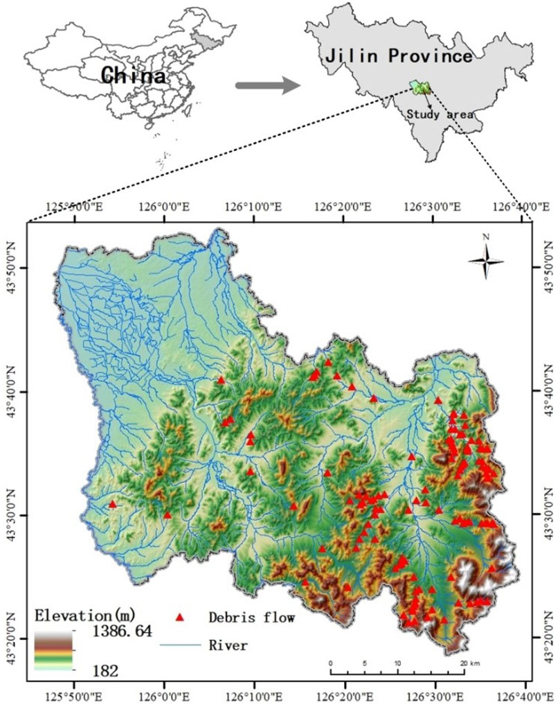
FIGURE 1. The geographic location of the study area.
The study area lies between 125°48′09″E to 126°40′01″E longitude and 43°18′07″N to 43°35′00″N latitude. There are four landforms in the entire area: middle mountains, low mountains, platform, and river valley. From southeast to northwest, the landforms of the study area are middle mountains, low mountains and platform with the altitudes ranging from 1,386 to 182 m. In addition to several andesites and metamorphic rocks, the main rock type is Yanshan Early Granite. The study area lies in the Tianshan–Xingan geosyncline fold area of the Jilin and Heilongjiang fold system (Qin et al., 2019). Folds and faults are relatively developed in Yongji county, which provides conditions for the occurrence of geological disasters (Figure 2A). Yongji county is in the mid-latitude subtemperate continental climate zone with an annual average precipitation of 722.75 mm. There are 39 rivers covering an area of more than 20 km2. The main rivers include the Yinma River, Wende River, Chalu River and Aolong River.
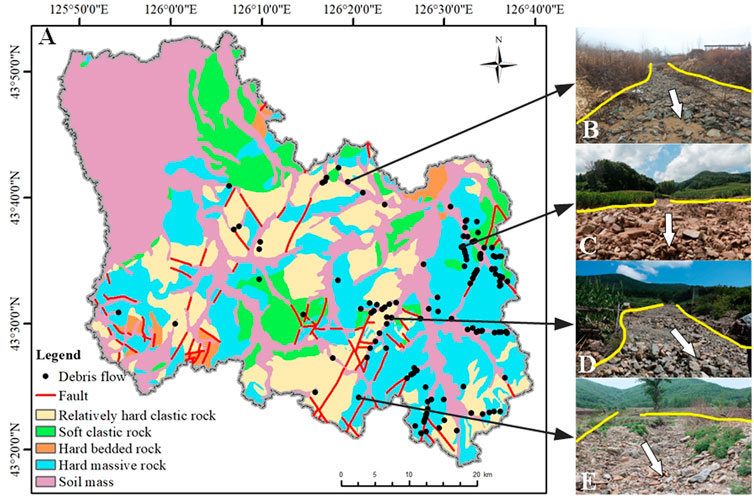
FIGURE 2. Geological map and debris flow field photos of the study area: (A) geological map; (B–E) debris flow field photos.
A debris flow inventory map is a prerequisite for DFSM(Xu et al., 2012; Arabameri et al., 2020; Dash et al., 2022). A total of 129 debris flows were collected based on field surveys and historical materials. Figure 2A shows that debris flows are mainly distributed across the southeast mountain area. Statistics show that among 129 debris flows, only 7 are medium in size and 122 are small. In recent years, the increase in debris flow frequency in Yongji county has been closely related to deforestation and reclamation. With the destruction of forest vegetation, rainfall is more likely to cause soil erosion, which gradually forms a series of gullies. These gullies provide circulation conditions for debris flows. Figures 2B–E shows some images of occurred debris flows in the study area.
In this study, the extraction of watershed units was completed in ArcGIS 10.2 software (Tien Bui et al., 2015; Cao et al., 2019). The most commonly used watershed units (HWUs) are classified by the hydrological principles (Fausto Guzzetti et al., 1999). HWUs are derived based on an 8-direction flow algorithm (Horton et al., 2013). Establishing the HWUs consists of the following six steps: 1) filling the original DEM, 2) extracting the flow direction, 3) calculating the flow accumulation, 4) extracting river networks based on a threshold, 5) stream linking, 6) dividing HWUs based on flow direction and stream linking. The detailed classification process is shown in Figure 3A.
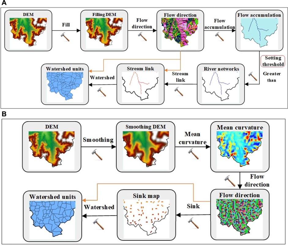
FIGURE 3. Classification process of the watershed units: (A) hydrological analysis method and (B) mean curvature method.
In addition, watershed units can be generated based on the mean curvature method (CWUs). The mean curvature is a simple combination of profile curvature and plan curvature. Its maximum and minimum values can indicate the changes in aspect and slope positions at the same time. Therefore, the mean curvature can reflect the ridge line, valley line, platform edge and wide valley edge (Romstad and Etzelmüller, 2012). Establishing the CWUs consists of the following five steps: 1) smoothing the original DEM, 2) calculating the mean curvature, 3) extracting the flow direction, 4) filling depressions based on flow direction data, and 5) dividing CWUs based on flow direction and depressions. The detailed classification process is shown in Figure 3B.
For HWUs, the number and size are closely related to DEM resolution and flow threshold, but for CWUs, the control factor is only DEM resolution. For HWUs, flow threshold values of 500, 1,000, 2000, 5,000, and 10,000 were chosen based on a DEM with a resolution of 30 m. For CWUs, we resampled the DEM with resolutions of 50, 100, 200, 300, 500, and 1,000. To ensure that the number and size of the two types of watershed units were not much different and consistent with the actual watersheds, a flow threshold of 1,000 and a DEM resolution of 300 were selected to divide the watershed units. For the HWUs, the study area was divided into 1,092 watershed units. The smallest unit was 0.10 km2, the largest unit was 13.63 km2, and the mean size was 2.40 km2 (Figure 4A). For CWUs, the study area was divided into 1,211 watershed units. The smallest unit was 0.11 km2, the largest unit was 8.87 km2, and the mean size was 2.17 km2 (Figure 4B).
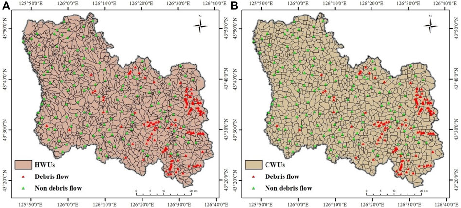
FIGURE 4. Division of watershed units: (A) hydrological analysis method and (B) mean curvature method.
The flowchart of the research methodology is shown in Figure 5. DFSM of Yongji county using four models (LR, MLP, CART, and BN) and watershed units (HWUs and CWUs) have been carried out in five main steps: 1) data collection and screening influencing factors, 2) division of two types of watershed units, 3) calculation of frequency ratio values (FRs) for all influencing factors, 4) building debris flow models and constructing DFSM, and 5) debris flow model validation and comparison using AUC, ACC and Kappa.
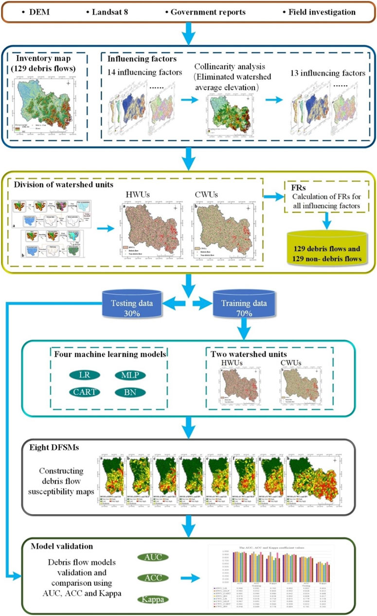
FIGURE 5. Flowchart of the research methodology.
The occurrence of debris flows is affected by many factors including topographic, geomorphologic, geological, ecological and meteorological factors (Zhang et al., 2012; Bregoli et al., 2014; Hu et al., 2014). Based on field observations, available literature and expert experience, fourteen influencing factors were considered, such as watershed area, relative height difference, watershed average elevation, watershed slope, mean curvature, fault density, river density, stream power index (SPI), topographic wetness index (TWI), plan normalized difference vegetation index (NDVI), landforms, precipitation, land use and lithology.
Because substantial collinearity will lead to model instability, collinearity analysis is essential before influencing factors are applied for DFSM(Qiu et al., 2022). Person’s correlation coefficient was calculated to test the collinear relationship among these factors, and the results are shown in Table 1. There is no correlation coefficient when the absolute value is less than 0.7 (Dormann et al., 2013; Yao et al., 2022). There was high collinearity between relative height difference and watershed average elevation, and the Person’s correlation coefficient was 0.86. In addition, the value of collinearity between watershed average elevation and precipitation was 0.69. Therefore, the watershed average elevation was eliminated.
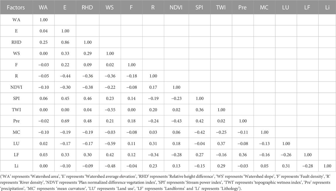
TABLE 1. The results of the Person’s Correlation Coefficient.
The watershed area, relative height difference, watershed slope, mean curvature, SPI and TWI were extracted from the DEM with a resolution of 30 m. Fault, river, and lithology data were acquired from the geological map of Yongji county and field investigations. The Landsat 8 image taken on 11 August 2021, was used to produce the NDVI. Landforms, precipitation, and land use were provided by government reports. Thirteen influencing factors were converted to a grid cell with a resolution of 30 m in ArcGIS 10.2 (Chen et al., 2017). Table 2 shows date source and scale of influencing factors. When watershed units are applied to DFSM, grid patterns for each factor need to be transferred to the corresponding watershed units. For watershed area, geometric calculation in the attribute table was used to calculate the area of each watershed. The difference between the highest and the lowest points in each watershed was calculated as a relative height difference (Qin et al., 2019). For watershed slope, mean curvature, SPI, TWI, and NDVI, the zonal statistics tool in the spatial analysis was used and the statistical type was “mean.” The length of faults and rivers in each watershed was extracted by using the intersection tool, and then, the fault density and river density in each watershed were calculated using the field calculator. Precipitation for each watershed was determined based on the principle of majority, and this principle was also applied to factors of landforms, land use and lithology. The data types of precipitation, landforms, land use and lithology are discrete, while the data types of other factors are continuous. The influencing factor layers based on HWUs with a flow threshold of 1,000 are shown in Figure 6.
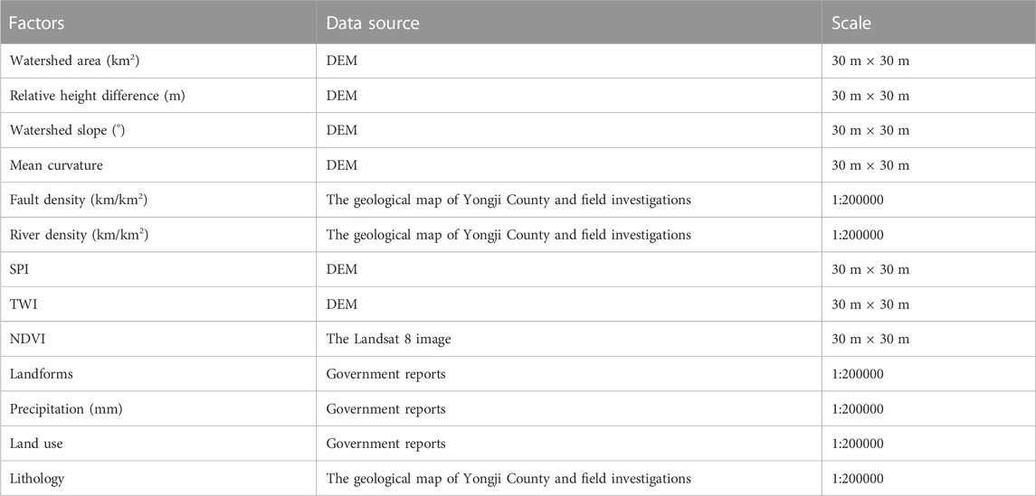
TABLE 2. Date source and scale of influencing factors.
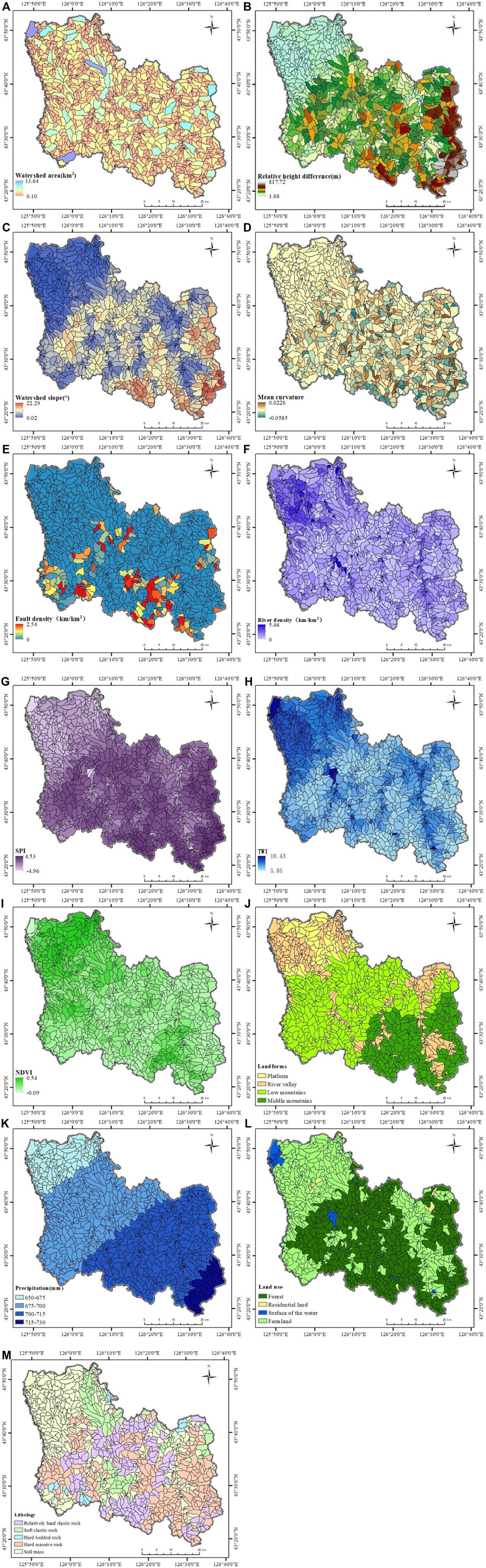
FIGURE 6. . Maps of influencing factors based on HWUs with a flow threshold of 1,000: (A) watershed area; (B) relative height difference; (C) watershed slope; (D) mean curvature; (E) fault density; (F) river density; (G) SPI; (H) TWI; (I) NDVI; (J) landforms; (K) precipitation; (L) land use; (M) lithology.
The FRs of the influencing factor subclass were used as the input variable of the DFSM models (Huang et al., 2020). Based on a series of previous studies (Xu et al., 2012; Aditian et al., 2018; Vakhshoori et al., 2019; Chang et al., 2020), we divided the continuous factor into eight levels using the natural fracture method. Taking HWUs with a flow threshold of 1,000 as an example, the FRs for each level of thirteen factors are shown in Table 3.
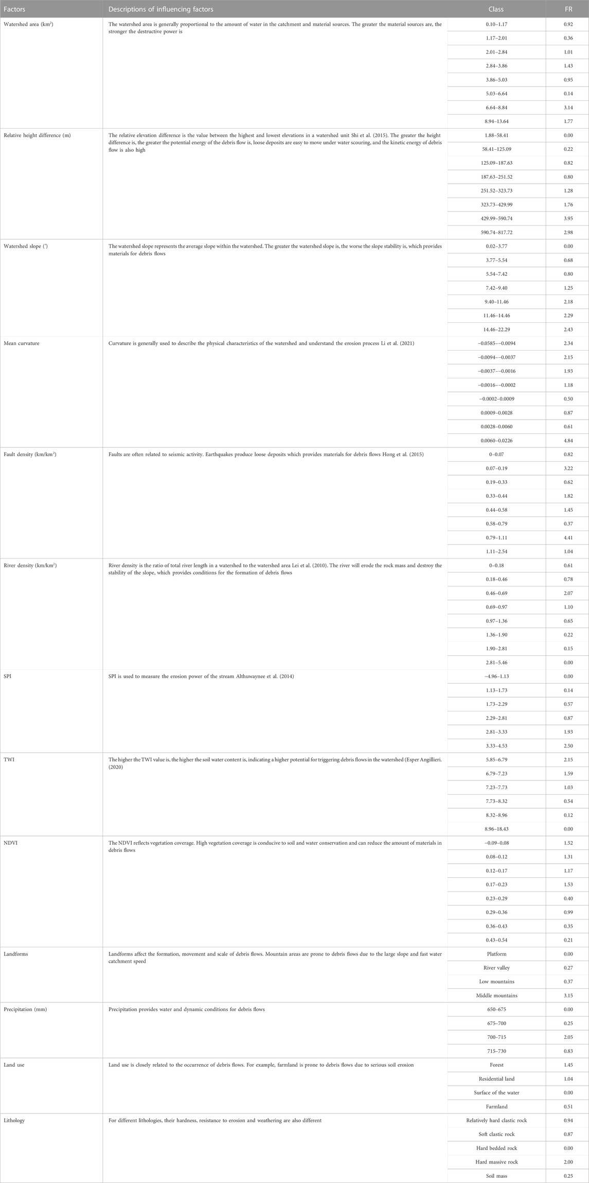
TABLE 3. Description and FRs of all the influencing factors (HWUs with a flow threshold of 1,000).
Logistic regression (LR) may be the most widely used statistical technique in susceptibility assessment (Colkesen et al., 2016). As a multivariate regression method, LR can find a model to describe the relationship between multiple independent variables and a dependent variable (Lee and Pradhan 2006; Lee 2007; Pourghasemi et al., 2013). For DFSM, the influencing factors are considered the independent variables and the occurrence and non-occurrence of debris flows are considered the dependent variables. For LR, variables may be continuous, discrete or arbitrary combinations of two types (Lee, 2007). LR can be expressed as follows (Ayalew and Yamagishi 2005; Yalcin et al., 2011; Schlögel et al., 2018):
where
Multilayer perceptron (MLP) is a kind of artificial neural network and has been widely used in classification (Tien Bui et al., 2015; Pham et al., 2017). The MLP generally consists of three main components, namely, input layers, hidden layers, and output layers (Kavzoglu and Mather 2003). For DFSM, the input layers are considered the influencing factors of debris flow, the output layers are considered the classification result of inferring debris flow or non-debris flow, and the hidden layers are considered the classification layers that convert input into output. The MLP model with only one hidden layer is the most basic three-tier structure model, which can fit and predict many non-linear problems (Li et al., 2019). In this study, a single-hidden-layer MLP model is used in DFSM. For example,
where
where
The decision tree model is a technique that uses a tree structure to discover and describe structural patterns in data. It does not require a preestablished relationship between all input variables and a target variable (Hitoshi Saito and Matsuyama, 2009). As an algorithm of the decision tree model, classification and regression tree (CART) was first proposed by Breiman et al. (1984) The CART consists of a root node, a set of internal nodes and a set of leaf nodes. The leaf nodes correspond to the classification result, and the other nodes correspond to the classification rules. CART was selected as the decision tree model in this study in view of its performance efficiency (Wang et al., 2015).
The Bayesian network (BN) is a graphical model for probabilistic relationships among a set of variables (Song et al., 2012). BN can be represented by directed acyclic graphs and conditional probabilities, reflecting the independent and interdependent relationship among various variables. The calculation formula is given as follows (Han et al., 2019):
where
In this study, three commonly used criteria, including the predictive accuracy (ACC), the Kappa coefficient and the area under the receiver operating characteristic curve (AUC) were used to evaluate the prediction ability of DFSMs. The calculation of the three criteria is based on the confusion matrix (Ghasemian et al., 2022a). The confusion matrix, also known as the error matrix, is a standard format for accuracy evaluation. The confusion matrix can represent the difference between the model prediction results and the actual observation results (Xiong et al., 2020). In this study, the confusion matrix of the debris flow susceptibility predictive models is shown in Table 4. For example, a true positive (TP) suggests that the prediction result is ‘Debris-Flow’, and the actual observation result is ‘Debris-Flow’.

TABLE 4. Confusion matrix.
The predictive accuracy (ACC) represents the ratio of correctly predicted observations to total observations. This index shows how well the debris flow model works:
The Kappa index is used to assess the acceptability of debris flow models which can be calculated by:
where
The receiver operating characteristic (ROC) curve and area under the curve (AUC) can compare the prediction performance of different classifiers (Akgun et al., 2012). The abscissa and ordinate of the ROC are the false-positive rate (FPR) and true-positive rate (TPR) respectively. They can be obtained from the following equations (Pourghasemi et al., 2013):
AUC represents the quality of models that reliably predict the occurrence or non-occurrence of debris flows. The AUC varies from 0.5 to 1.0, and the higher the AUC value is, the better the prediction performance of the model.
The whole analysis process was implemented in IBM SPSS software (Sun et al., 2019; Sun et al., 2021). For LR, the forward step mode was adopted to screened variables. For BN model, the mechanism type was Tree Augmented naive Bayes (TAN), and Bayesian adjustment of small cell count was selected as a parameter learning method. For MLP, one hidden layer was selected, and the maximum training time was used as the termination rule. For CART, the maximum tree depth was set to 10, and percentage was used as the termination rule. Other parameters are default.
The Chi-Squared statistic was employed to identify the most important factors affecting the occurrence of debris flows in the study area (Ghasemian et al., 2022a). Figure 7 shows that landforms have the highest impact (128.5) on debris flows in the study area, followed by relative height difference and SPI (114.5), watershed slope (110.5), TWI (82.5), precipitation (74.5), lithology (60), land use (43.5), watershed area (27.5), river density (26.5), mean curvature (24), NDVI (23), and fault density (21.5).
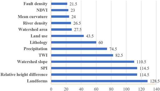
FIGURE 7. Contribution of influencing factors.
According to field surveys and historical materials, a total of 129 debris flows were collected. Meanwhile, 129 non-debris flows were selected, which were at least 500 m away from the nearest debris flow (Figure 4) (Dou et al., 2019; Sun et al., 2020). Assigned 1 and 0 for debris flows and non-debris flows, respectively. The FRs of the thirteen influencing factors shown in Table 2 were taken as the input variables, and the debris flows and non-debris flows were taken as the output variables. For all 258 samples, 70% (n = 180) were selected randomly for training data, which were used to create the DFSM models. The remaining 30% (n = 78) were used as testing data, which were applied to validate the DFSM models. Based on two types of watershed units (HWUs and CWUs) and four models (LR, MLP, CART and BN), eight DFSMs of Yongji county were completed.
In this paper, IBM SPSS software was chosen to build the debris flow susceptibility predictive models. The model outputs are the debris flow susceptibility indices of all watershed units in the study area. Debris flow susceptibility indices are the probability of debris flow occurrence which varies from 0 to 1 (Xiong et al., 2020). Based on the ArcGIS software, the debris flow susceptibility indices were converted into raster format to produce the debris flow susceptibility map. Quantile classification was applied to divide the final maps into five classes, namely, very low susceptibility (VL), low susceptibility (L), moderate susceptibility (M), high susceptibility (H), and very high susceptibility (VH). (Martha et al., 2013; Hussin et al., 2016; Steger et al., 2017).
As shown in Figure 8, the susceptibility distributions of the eight models have common characteristics. Very high and high susceptibility areas are mainly distributed in the southeast, moderate susceptibility areas are mainly distributed in the middle, and very low and low susceptibility areas are mainly distributed in northwestern of Yongji county, which is consistent with previous research results (Qin et al., 2019). The landform in the southeast of the study area is mainly middle mountains, and the land use is mainly forest and farmland. The watershed units distributed in the southeast have large relative height differences and slopes, which leads to frequent debris flow disasters. The precipitation decreases from southeast to northwest, which is consistent with the susceptibility distribution. The lithology in southeastern Yongji county is hard massive rock, mainly granite. Weathered granite is a component of debris flows, which increases the density and destructive power of debris flows (Figures 2B–E).
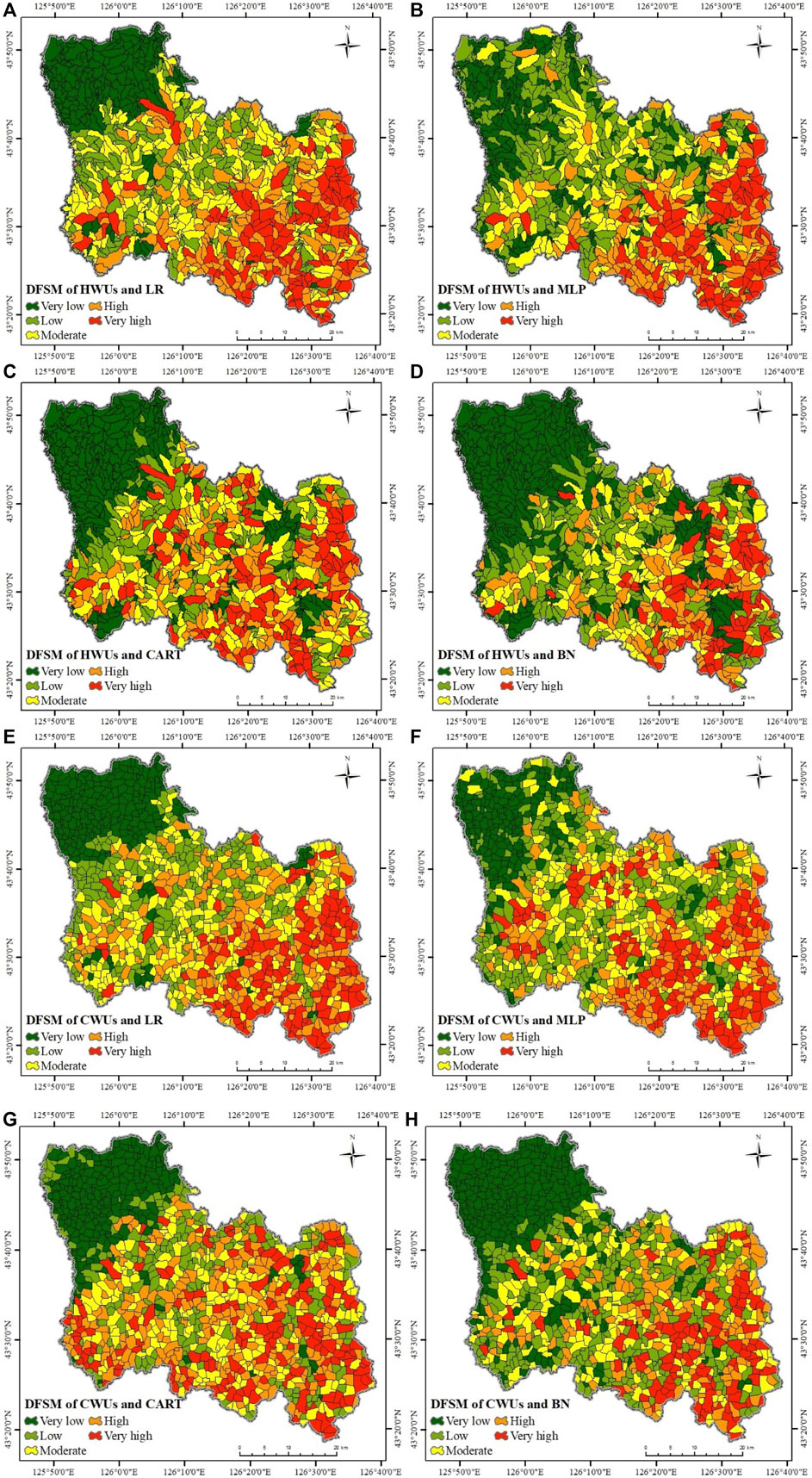
FIGURE 8. Eight DFSMs: (A) DFSM of HWUs and LR; (B) DFSM of HWUs and MLP; (C) DFSM of HWUs and CART; (D) DFSM of HWUs and BN; (E) DFSM of CWUs and LR; (F) DFSM of CWUs and MLP; (G) DFSM of CWUs and CART and (H) DFSM of CWUs and BN.
For the eight DFSMs, the area ratios of the five susceptibility classes (very high, high, moderate, low, and very low) were 12.85–19.96, 13.82–21.51, 14.87–23.79, 17.70–28.33, and 16.56%–36.70%, respectively (Figure 9A); The debris flow ratios of the five susceptibility classes were 62.79–76.74, 12.40–24.81, 6.98–14.73,0.78%–3.10% and 0%–0.78%, respectively (Figure 9B). As shown in Figure 9C, the debris flow density was calculated to evaluate the performance of the DFSMs, that is, the ratio of debris flow percentage to area percentage on each susceptible class (Pham et al., 2016). The maximum values of the debris flow density of the eight models appear in the very high susceptibility class, varying from 3.15 to 5.61. The minimum values all appear in the very low susceptibility class, varying from 0.00 to 0.04. The debris flow density increases gradually from a very low class to a very high class, which provides a good visualization of the spatial predictions of debris flows (Pham et al., 2017; Asadi et al., 2022).
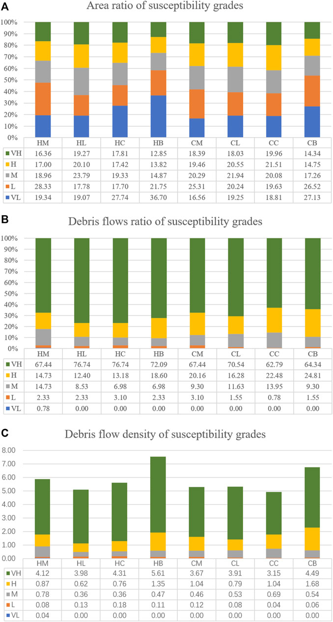
FIGURE 9. The classification of DFSMs and debris flow density: (A) area ratio; (B) debris flows ratio; (C) debris flow density.
Model validation is a vital step in disaster susceptibility mapping (Wang et al., 2022). By considering the three commonly used performance metrics of ACC, AUC and Kappa, eight models were verified. The AUC, ACC and Kappa coefficient values of the eight models on the training and testing data are shown in Figure 10.
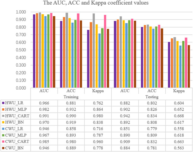
FIGURE 10. The AUC, ACC, and Kappa coefficient values of the eight models for the training and testing data.
In the training phase, when HWUs were used as the mapping unit, the ACC stated that HWUs_CART model had the highest value (0.990), followed by HWUs_MLP (0.932), HWUs_BN (0.919) and HWUs_LR (0.881). It showed that the HWUs_CART model can correctly classify the debris flow and non-debris flow locations as debris flow and non-debris flow situations respectively. The highest and lowest Kappa values were 0.980 and 0.762, respectively for the HWUs_CART and HWUs_LR. Meanwhile, HWUs_MLP (0.864) and HWUs_BN (0.838) was ranked in other positions. In terms of AUC, results indicated that the HWUs_CART model with a value of 0.991 had higher performance than the HWUs_MLP (0.982), HWUs_BN (0.970) and HWUs_LR (0.966). When CWUs was used as the mapping unit, the ACC, Kappa and AUC values of the CWUs_CART model were 0.980, 0.960 and 0.985, which showed that the performance of the CWUs_CART model was the highest, followed by the CWUs_MLP (0.893, 0.787, 0.967), CWUs_BN (0.899, 0.778, and 0.946) and CWUs_LR (0.858, 0.716, and 0.946) (Figure 10). Although the results showed the excellent performance for all the four algorithms, the CART had the highest ability in debris flow classification and susceptibility mapping in the study area. In terms of watershed unit, ACC, Kappa and AUC values decreased when HWUs was replaced by CWUs, indicating that HWUs were more suitable for DFSM in the study area than CWUs.
Right side of Figure 10 showed the prediction capabilities of the eight models based on testing dataset. These results are very important for evaluating the applicability and robustness of the models. When HWUs were used as the mapping unit, the highest value of ACC was 0.834 for the HWUs_CART model, next for the HWUs_MLP (0.826), HWUs_BN (0.808) and HWUs_LR (0.802) models. The Kappa for the HWUs_CART model was 0.668 as the highest value, whereas this value was 0.652, 0.617, and 0.604 for HWUs_MLP, HWUs_BN, and HWUs_LR, respectively. The highest and lowest AUC values were 0.942 and 0.882, respectively for the HWUs_CART and HWUs_LR. Meanwhile, HWUs_MLP (0.902) and HWUs_BN (0.892) was ranked in other positions. Correspondingly, ACC, Kappa and AUC from CWUs were shown in Figure 9, which indicated a similar result with HWUs. CART model resulted in the highest ACC, Kappa and AUC values of 0.832, 0.663, and 0.909, which manifested it is the best model for the study area. At the same time, the HWU-based models had better performance than the CWU models for DFSM in the study area.
The results of the models are tested by one-way ANOVA in SPSS. For HWUs, there are significant differences between CART and each of the three methods (LR, MLP, and BN). There are no significant differences among LR, MLP, and BN. For CWUs, there are no significant differences between MLP and each of the two methods (LR and BN). There are significant differences between the other methods.
As shown in Figure 3, the extraction processes of HWUs are more complex than those of CWUs, because HWUs require six steps while CWUs require five steps. Model builder in ArcGIS is a workflow that connects a series of geoprocessing tools (Qin et al., 2019). It takes the output of one tool as the input of the other tool. Model builder can greatly reduce operation time and improve work efficiency. We had built two workflows for the processes of extracting HWUs and CWUs in the model builder. Experiments on two types of watershed units showed that HWUs extraction required 17 s, while CWUs extraction required only 3 s. In addition, for the division of HWUs, the influence of DEM resolution and flow threshold needs to be considered, while for CWUs, only DEM resolution needs to be considered. In summary, it takes more time and effort to extract HWUs than CWUs.
There are also significant differences between the two types of watershed units in the classification results. As shown in Figure 4, HWUs are mostly strip-shaped and widely different in size, while CWUs are nearly square and relatively uniform in size. The watershed unit boundaries extracted by the hydrological analysis method in areas with obvious topographic changes are relatively consistent with reality (Figure 11A). However, there are many small and narrow units in flat areas, because there is no clear flow direction in flat areas for hydrological analysis (Massimiliano et al., 2016) (Figure 11C). For the curvature method, the division of watershed units in flat areas is relatively satisfactory, and there is no parallel line problem similar to the hydrological analysis method (Figure 11D). However, in areas with obvious topographic changes, the boundaries of watershed units do not match well with the actual situation (Figure 11B).
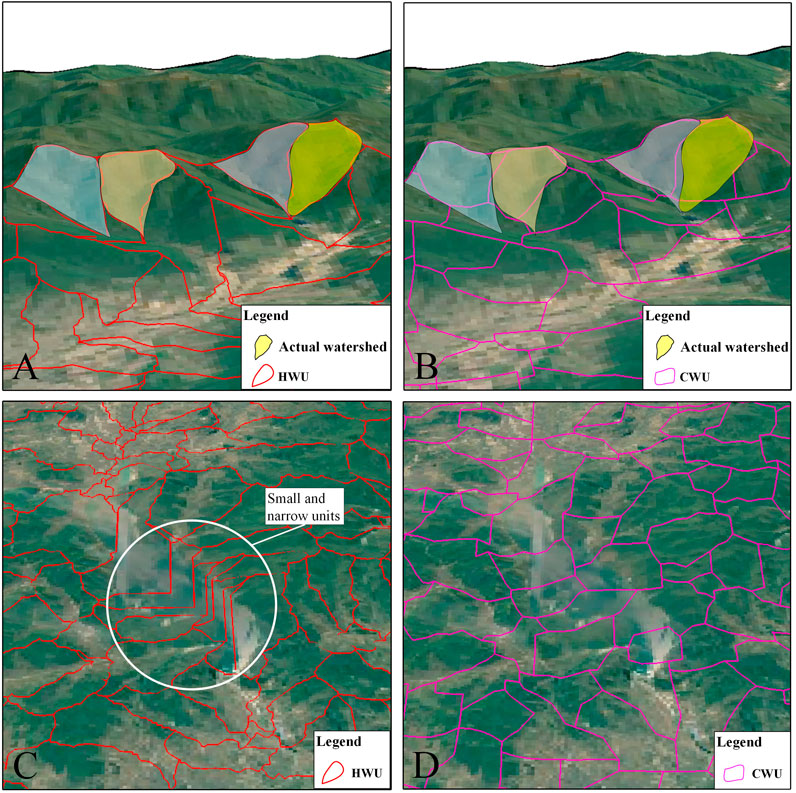
FIGURE 11. Watershed unit classification results comparison: (A) The boundaries of HWUs are relatively consistent with reality in mountainous areas; (B) The boundaries of CWUs do not match well with the actual situation in mountainous areas; (C) Small and narrow units in flat areas of HWUs; and (D) The division of CWUs in flat areas is relatively satisfactory.
Four models, LR, MLP, CART and BN, were used to complete the DFSMs of Yongji county in this study. Figure 10 shows the predictive ability of the eight models. When HWUs were used as mapping units, CART had the highest evaluation criteria with AUC, ACC and Kappa values of 0.991, 0.990, and 0.980 respectively, followed by MLP (0.982, 0.932, 0.864), BN (0.970, 0.919, 0.838) and LR (0.966, 0.881, 0.762) in the training stage. For the testing stage, the CART had the highest prediction accuracy with AUC, ACC and Kappa values of 0.942, 0.834 and 0.668 respectively, followed by MLP (0.902, 0.826, 0.652), BN (0.892, 0.808, 0.617) and LR (0.882, 0.802, 0.604). When CWUs were used as mapping units, the evaluation results showed the same trend as HWUs. The comparisons of the four evaluation models show that the CART had the best predictive ability over the other three models. The current research was in agreement with previous research results. Wang et al. (2015) analyzed landslide susceptibility based on five mathematical models (artificial neural network, frequency ratio, CART, LR and weights of evidence methods) and three sampling strategies. They indicated the results obtained from CART show steady prediction power with an AUC value larger than 0.7. Felicísimo et al. (2012) indicated that the CART is one of the most predictive models with the AUC value of 0.77. Using random forest (RF), boosted regression tree (BRT), classification and regression tree (CART), and general linear (GLM), Youssef et al. (2015) found the success rate for CART was 0.816 and for the prediction rate the CART was the highest with a value of 0.862. CART represents information in an intuitive and easy visual way, and is widely used in many fields (Bevilacqua et al., 2003; Malinowska 2014; Kim et al., 2015; Youssef et al., 2015; Yang et al., 2016).
Several studies have been conducted in similar areas. Selecting the frequency ratio (FR) model as the statistical method, Qin et al. (2019) explored the accuracy and practicability of HWUs and grid cell units (GCUs) in evaluating debris flow susceptibility in Yongji county. Qiao et al. (2021) built debris flow susceptibility models via the analytical hierarchy process (AHP) method and generated maps of Yongji county. The AUC values of the testing data in different studies are shown in Table 5. When the HWUs were chosen as mapping units, the AUC values of the DFSMs based on AHP, FR, LR, BN, MLP and CART were 0.812, 0.879, 0.882, 0.892, 0.902, and 0.942 respectively. The main difference among these DFSMs is the selection of different evaluation models, which indicates that machine learning models can improve the prediction accuracy of DFSMs. These results are consistent with previous studies, indicating that machine learning models are more suitable for DFSM than heuristic and general statistical models (Huang et al., 2020; Sun et al., 2021).
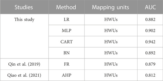
TABLE 5. AUC values of testing data in different studies.
The selection of mapping units is one of the key issues for the rationality and correctness of disaster susceptibility mapping (Van Den Eeckhaut et al., 2009; Chen et al., 2019; Sun et al., 2020). The impact of different mapping units on disaster susceptibility mapping is greater than that of statistical methods (Zezere et al., 2017). Although many studies have tried to compare different evaluation models for disaster susceptibility mapping (Achour et al., 2018; Liang et al., 2020; Xiong et al., 2020; Dash et al., 2022; Qiu et al., 2022), very few studies have considered different mapping units. Qin et al. (Qin et al., 2019) explored the effect of grid cell unit and HWUs on the susceptibility mapping of debris flow, they found HWUs can reflect the geological and geomorphic environmental conditions of a debris flow accurately and perfectly. Li et al. (Li et al., 2021) discussed the influence of four different HWUs on debris flow susceptibility assessment results. The results show that the appropriate watershed division scheme can obtain more reasonable results. In this study, HWUs and CWUs were selected to map debris flow susceptibility. When the CART was selected as the machine learning model, the HWUs generated high AUC, ACC, and Kappa for training data (0.991, 0.990 and 0.980) compared to the CWUs (0.985, 0.980, and 0.960). For testing data, the AUC, ACC, and Kappa of HWUs were 0.942, 0.834, and 0.668, respectively. The AUC, ACC, and Kappa of CWUs were 0.909, 0.832, and 0.663, respectively. The results suggest that the HWU model has a higher debris flow prediction performance than the CWU model. The same trend can be observed in the LR, MLP, and BN models. Therefore, the HWU-based model is superior to the CWU-based model in debris flow susceptibility assessment due to higher training and testing accuracy.
As described in “6.1 Watershed unit classification processes and results comparison,” compared with CWUs, HWUs agree well with the actual watershed units in mountainous areas, but small and narrow units appear in plain areas. Since the frequency of debris flows in mountainous areas is much higher than that in plain areas, the division of watershed units in mountainous areas is more important than that in plain areas. Therefore, the HWU model is more practical than the CWU model. CWUs can also represent the distribution of watersheds and can be used as an alternative scheme.
Although this paper discussed the application of two types of watershed units in DFSM and obtained positive results, there are some limitations: 1) the number of debris flows is small, and 2) only HWUs with a threshold of 1,000 and CWUs with a resolution of 300 are selected for comparison. In future research, we will constantly update the debris flow database to improve the data quality. Moreover, it is necessary to explore the similarities and differences of multiscale watershed units in DFSM.
This paper mainly explored the influence of using different watershed units (HWUs and CWUs) in debris flow susceptibility assessment models. LR, MLP, CART, and BN were chosen as evaluation models to avoid the model uncertainty caused by different models. Yongji county, with 129 recorded debris flows and 13 related influencing factors, was used as the study area and eight DFSMs were produced.
The DFSM results showed that CART has the best predictive ability over the other three models through the analysis of AUC, ACC and Kappa. By using Model Builder in ArcGIS, 1,092 HWUs and 1,211 CWUs were extracted. Compared with HWUs, the extraction process of CWUs is simpler. For the results of watershed unit division, HWUs have more advantages in areas with undulating terrain, but they are not satisfactory in areas with flat terrain. CWUs perform well in flat areas but do not match the actual watershed boundaries in areas with undulating terrain. Since debris flows mostly occur in mountainous areas, the DFSM based on HWUs is more accurate and practical than that based on CWUs. In addition, the AUC, ACC and Kappa showed that the HWU-based model has remarkably higher debris flow prediction performance than CWUs. This result means that the HWUs are more effective in debris flow susceptibility assessment of the study area. The CWU-based model can also reflect the spatial distribution probability of debris flows in the study area overall and can be used as an alternative model. Further studies should propose a more appropriate watershed unit for DFSM.
The original contributions presented in the study are included in the article/supplementary material, further inquiries can be directed to the corresponding author.
JL: Conceptualization, methodology, formal analysis, investigation, writing, original draft, writing-review and editing. SUQ: Methodology, validation, resources, data curation, writing -original draft, visualization, project administration, funding acquisition. JC: Validation, investigation, supervision, project administration. SGQ: Investigation, supervision. JGY: Software, data curation. XZ: Conceptualization, supervision. RC: Software, supervision. JHY: Investigation, data curation.
This work was funded by the National Natural Science Foundation of China under Grants 41977221 and 41972267, and in part by the Jilin Provincial Science and Technology Department (Grant No. 20190303103SF).
The authors are also thankful to the reviewers for their valuable feedback on the manuscript.
JL, XZ, RC, and JHY were employed by China Water Resources Bei Fang Investigation, Design & Research Co. LTD.
The remaining authors declare that the research was conducted in the absence of any commercial or financial relationships that could be construed as a potential conflict of interest.
All claims expressed in this article are solely those of the authors and do not necessarily represent those of their affiliated organizations, or those of the publisher, the editors and the reviewers. Any product that may be evaluated in this article, or claim that may be made by its manufacturer, is not guaranteed or endorsed by the publisher.
Achour, Y., Garçia, S., and Cavaleiro, V. (2018). GIS-based spatial prediction of debris flows using logistic regression and frequency ratio models for Zêzere River basin and its surrounding area, Northwest Covilhã, Portugal. Arabian J. Geosciences 11, 550. doi:10.1007/s12517-018-3920-9
Aditian, A., Kubota, T., and Shinohara, Y. (2018). Comparison of GIS-based landslide susceptibility models using frequency ratio, logistic regression, and artificial neural network in a tertiary region of Ambon, Indonesia. Geomorphology 318, 101–111. doi:10.1016/j.geomorph.2018.06.006
Akgun, A., Kincal, C., and Pradhan, B. (2012). Application of remote sensing data and GIS for landslide risk assessment as an environmental threat to Izmir city (west Turkey). Environ. Monit. Assess. 184, 5453–5470. doi:10.1007/s10661-011-2352-8
Althuwaynee, O. F., Pradhan, B., Park, H. J., and Lee, J. H. (2014). A novel ensemble decision tree-based CHi-squared Automatic Interaction Detection (CHAID) and multivariate logistic regression models in landslide susceptibility mapping. Landslides 11, 1063–1078. doi:10.1007/s10346-014-0466-0
Arabameri, A., Saha, S., Roy, J., Chen, W., Blaschke, T., and Tien Bui, D. (2020). Landslide susceptibility evaluation and management using different machine learning methods in the gallicash river watershed, Iran. Remote Sens. 12, 475. doi:10.3390/rs12030475
Asadi, M., Goli Mokhtari, L., Shirzadi, A., Shahabi, H., and Bahrami, S. (2022). A comparison study on the quantitative statistical methods for spatial prediction of shallow landslides (case study: Yozidar-Degaga Route in Kurdistan Province, Iran). Environ. Earth Sci. 81, 51. doi:10.1007/s12665-021-10152-4
Ayalew, L., and Yamagishi, H. (2005). The application of GIS-based logistic regression for landslide susceptibility mapping in the Kakuda-Yahiko Mountains, Central Japan. Geomorphology 65, 15–31. doi:10.1016/j.geomorph.2004.06.010
Balamurugan, G., Ramesh, V., and Touthang, M. (2016). Landslide susceptibility zonation mapping using frequency ratio and fuzzy gamma operator models in part of NH-39, Manipur, India. Nat. Hazards 84, 465–488. doi:10.1007/s11069-016-2434-6
Bălteanu, D., Chendeş, V., Sima, M., and Enciu, P. (2010). A country-wide spatial assessment of landslide susceptibility in Romania. Geomorphology 124, 102–112. doi:10.1016/j.geomorph.2010.03.005
Bevilacqua, M., Braglia, M., and Montanari, R. (2003). The classification and regression tree approach to pump failure rate analysis. Reliab. Eng. Syst. Saf. 79, 59–67. doi:10.1016/s0951-8320(02)00180-1
Bregoli, F., Medina, V., Chevalier, G., Hürlimann, M., and Bateman, A. (2014). Debris-flow susceptibility assessment at regional scale: Validation on an alpine environment. Landslides 12, 437–454. doi:10.1007/s10346-014-0493-x
Breiman, L. F. F., Olshen, R., and Stone, C. (1984). Classification and regression trees. Wadsworth. Biometrics 40, 358.
Cama, M., Conoscenti, C., Lombardo, L., and Rotigliano, E. (2016). Exploring relationships between grid cell size and accuracy for debris-flow susceptibility models: A test in the giampilieri catchment (sicily, Italy). Environ. Earth Sci. 75, 238. doi:10.1007/s12665-015-5047-6
Cao, J., Zhang, Z., Wang, C., Liu, J., and Zhang, L. (2019). Susceptibility assessment of landslides triggered by earthquakes in the Western Sichuan Plateau. Catena 175, 63–76. doi:10.1016/j.catena.2018.12.013
Carranza, E. J. M. (2014). Data-Driven evidential belief modeling of mineral potential using few prospects and evidence with missing values. Nat. Resour. Res. 24, 291–304. doi:10.1007/s11053-014-9250-z
Chang, Z., Du, Z., Zhang, F., Huang, F., Chen, J., Li, W., et al. (2020). Landslide susceptibility prediction based on remote sensing images and GIS: Comparisons of supervised and unsupervised machine learning models. Remote Sens. 12, 502. doi:10.3390/rs12030502
Chen, J., Dai, Z., Dong, S., Zhang, X., Sun, G., Wu, J., et al. (2022). Integration of deep learning and information theory for designing monitoring networks in heterogeneous aquifer systems. Water Resour. Res. 58, 429. doi:10.1029/2022wr032429
Chen, J., Dai, Z., Yang, Z., Pan, Y., Zhang, X., Wu, J., et al. (2021). An improved tandem neural network architecture for inverse modeling of multicomponent reactive transport in porous media. Water Resour. Res. 57, 595. doi:10.1029/2021wr030595
Chen, W., Shahabi, H., Shirzadi, A., Hong, H., Akgun, A., Tian, Y., et al. (2018). Novel hybrid artificial intelligence approach of bivariate statistical-methods-based kernel logistic regression classifier for landslide susceptibility modeling. Bull. Eng. Geol. Environ. 78, 4397–4419. doi:10.1007/s10064-018-1401-8
Chen, W., Xie, X., Wang, J., Pradhan, B., Hong, H., Bui, D. T., et al. (2017). A comparative study of logistic model tree, random forest, and classification and regression tree models for spatial prediction of landslide susceptibility. Catena 151, 147–160. doi:10.1016/j.catena.2016.11.032
Chen, Z., Liang, S., Ke, Y., Yang, Z., and Zhao, H. (2019). Landslide susceptibility assessment using different slope units based on the evidential belief function model. Geocarto Int. 35, 1641–1664. doi:10.1080/10106049.2019.1582716
Colkesen, I., Sahin, E. K., and Kavzoglu, T. (2016). Susceptibility mapping of shallow landslides using kernel-based Gaussian process, support vector machines and logistic regression. J. Afr. Earth Sci. 118, 53–64. doi:10.1016/j.jafrearsci.2016.02.019
Constantin, M., Bednarik, M., Jurchescu, M. C., and Vlaicu, M. (2010). Landslide susceptibility assessment using the bivariate statistical analysis and the index of entropy in the Sibiciu Basin (Romania). Environ. Earth Sci. 63, 397–406. doi:10.1007/s12665-010-0724-y
Dash, R. K., Falae, P. O., and Kanungo, D. P. (2022). Debris flow susceptibility zonation using statistical models in parts of northwest Indian himalayas—Implementation, validation, and comparative evaluation. Nat. Hazards 111, 2011–2058. doi:10.1007/s11069-021-05128-3
Devkota, K. C., Regmi, A. D., Pourghasemi, H. R., Yoshida, K., Pradhan, B., Ryu, I. C., et al. (2012). Landslide susceptibility mapping using certainty factor, index of entropy and logistic regression models in GIS and their comparison at Mugling–Narayanghat road section in Nepal Himalaya. Nat. Hazards 65, 135–165. doi:10.1007/s11069-012-0347-6
Dormann, C. F., Elith, J., Bacher, S., Buchmann, C., Carl, G., Carré, G., et al. (2013). Collinearity: A review of methods to deal with it and a simulation study evaluating their performance. Ecography 36, 27–46. doi:10.1111/j.1600-0587.2012.07348.x
Dou, J., Yunus, A. P., Tien Bui, D., Merghadi, A., Sahana, M., Zhu, Z., et al. (2019a). Assessment of advanced random forest and decision tree algorithms for modeling rainfall-induced landslide susceptibility in the Izu-Oshima Volcanic Island, Japan. Sci. Total Environ. 662, 332–346. doi:10.1016/j.scitotenv.2019.01.221
Dou, Q., Qin, S., Zhang, Y., Ma, Z., Chen, J., Qiao, S., et al. (2019b). A method for improving controlling factors based on information fusion for debris flow susceptibility mapping: A case study in Jilin Province, China. Entropy (Basel) 21, 695. doi:10.3390/e21070695
Dragut, L., and Eisank, C. (2011). Object representations at multiple scales from digital elevation models. Geomorphol. (Amst) 129, 183–189. doi:10.1016/j.geomorph.2011.03.003
Du, G., Zhang, Y., Yang, Z., Guo, C., Yao, X., and Sun, D. (2018). Landslide susceptibility mapping in the region of eastern himalayan syntaxis, Tibetan plateau, China: A comparison between analytical hierarchy process information value and logistic regression-information value methods. Bull. Eng. Geol. Environ. 78, 4201–4215. doi:10.1007/s10064-018-1393-4
Esper Angillieri, M. Y. (2020). Debris flow susceptibility mapping using frequency ratio and seed cells, in a portion of a mountain international route, Dry Central Andes of Argentina. Catena 189, 104504. doi:10.1016/j.catena.2020.104504
Fausto Guzzetti, A. C., Cardinali, M., Reichenbach, P., and Reichenbach, P. (1999). Landslide hazard evaluation: A review of current techniques and their application in a multi-scale study, central Italy. Geomorphology 31, 181–216. doi:10.1016/S0169-555X(99)00078-1
Felicísimo, Á. M., Cuartero, A., Remondo, J., and Quirós, E. (2012). Mapping landslide susceptibility with logistic regression, multiple adaptive regression splines, classification and regression trees, and maximum entropy methods: A comparative study. Landslides 10, 175–189. doi:10.1007/s10346-012-0320-1
Ghasemian, B., Shahabi, H., Shirzadi, A., Al-Ansari, N., Jaafari, A., Geertsema, M., et al. (2022a). Application of a novel hybrid machine learning algorithm in shallow landslide susceptibility mapping in a mountainous area. Front. Environ. Sci. 10, 897254. doi:10.3389/fenvs.2022.897254
Ghasemian, B., Shahabi, H., Shirzadi, A., Al-Ansari, N., Jaafari, A., Kress, V. R., et al. (2022b). A robust deep-learning model for landslide susceptibility mapping: A case study of kurdistan Province, Iran. Sensors (Basel) 22, 1573. doi:10.3390/s22041573
Hadmoko, D. S., Lavigne, F., and Samodra, G. (2017). Application of a semiquantitative and GIS-based statistical model to landslide susceptibility zonation in Kayangan Catchment, Java, Indonesia. Nat. Hazards 87, 437–468. doi:10.1007/s11069-017-2772-z
Han, L., Zhang, J., Zhang, Y., and Lang, Q. (2019). Applying a series and parallel model and a bayesian networks model to produce disaster chain susceptibility maps in the changbai mountain area, China. Water 11, 2144. doi:10.3390/w11102144
He, S., Pan, P., Dai, L., Wang, H., and Liu, J. (2012). Application of kernel-based Fisher discriminant analysis to map landslide susceptibility in the Qinggan River delta, Three Gorges, China. Geomorphology 171-172, 30–41. doi:10.1016/j.geomorph.2012.04.024
Hitoshi Saito, D. N., and Matsuyama, H. (2009). Comparison of landslide susceptibility based on a decision-tree model and actual landslide occurrence: The Akaishi Mountains, Japan. Geomorphology 109, 108–121. doi:10.1016/j.geomorph.2009.02.026
Hong, H., Pourghasemi, H. R., and Pourtaghi, Z. S. (2016). Landslide susceptibility assessment in lianhua county (China): A comparison between a random forest data mining technique and bivariate and multivariate statistical models. Geomorphology 259, 105–118. doi:10.1016/j.geomorph.2016.02.012
Hong, H., Pradhan, B., Xu, C., and Tien Bui, D. (2015). Spatial prediction of landslide hazard at the Yihuang area (China) using two-class kernel logistic regression, alternating decision tree and support vector machines. Catena 133, 266–281. doi:10.1016/j.catena.2015.05.019
Hong, H., Tsangaratos, P., Ilia, I., Loupasakis, C., and Wang, Y. (2020). Introducing a novel multi-layer perceptron network based on stochastic gradient descent optimized by a meta-heuristic algorithm for landslide susceptibility mapping. Sci. Total Environ. 742, 140549. doi:10.1016/j.scitotenv.2020.140549
Horton, P., Jaboyedoff, M., Rudaz, B., and Zimmermann, M. (2013). Flow-R, a model for susceptibility mapping of debris flows and other gravitational hazards at a regional scale. Nat. Hazards Earth Syst. Sci. 13, 869–885. doi:10.5194/nhess-13-869-2013
Hu, W., Xu, Q., Rui, C., Huang, R. Q., van Asch, T. W. J., Zhu, X., et al. (2014). An instrumented flume to investigate the initiation mechanism of the post-earthquake huge debris flow in the southwest of China. Bull. Eng. Geol. Environ. 74, 393–404. doi:10.1007/s10064-014-0627-3
Huang, F., Cao, Z., Guo, J., Jiang, S. H., Li, S., and Guo, Z. (2020). Comparisons of heuristic, general statistical and machine learning models for landslide susceptibility prediction and mapping. Catena 191, 104580. doi:10.1016/j.catena.2020.104580
Hussin, H. Y., Zumpano, V., Reichenbach, P., Sterlacchini, S., Micu, M., van Westen, C., et al. (2016). Different landslide sampling strategies in a grid-based bi-variate statistical susceptibility model. Geomorphology 253, 508–523. doi:10.1016/j.geomorph.2015.10.030
Ilia, I., and Tsangaratos, P. (2015). Applying weight of evidence method and sensitivity analysis to produce a landslide susceptibility map. Landslides 13, 379–397. doi:10.1007/s10346-015-0576-3
Jaafari, A., Panahi, M., Pham, B. T., Shahabi, H., Bui, D. T., Rezaie, F., et al. (2019). Meta optimization of an adaptive neuro-fuzzy inference system with grey wolf optimizer and biogeography-based optimization algorithms for spatial prediction of landslide susceptibility. Catena 175, 430–445. doi:10.1016/j.catena.2018.12.033
Jiang, H., Zou, Q., Zhou, B., Hu, Z., Li, C., Yao, S., et al. (2022). Susceptibility assessment of debris flows coupled with ecohydrological activation in the eastern qinghai-tibet plateau. Remote Sens. 14, 1444. doi:10.3390/rs14061444
Kavzoglu, T., and Mather, P. M. (2003). The use of backpropagating artificial neural networks in land cover classification. Int. J. Remote Sens. 24, 4907–4938. doi:10.1080/0143116031000114851
Kim, K. N., Kim, D. W., and Jeong, M. A. (2015). The usefulness of a classification and regression tree algorithm for detecting perioperative transfusion-related pulmonary complications. Transfusion 55, 2582–2589. doi:10.1111/trf.13202
Lee, S. (2007). Application of logistic regression model and its validation for landslide susceptibility mapping using GIS and remote sensing data. Int. J. Remote Sens. 26, 1477–1491. doi:10.1080/01431160412331331012
Lee, S., and Pradhan, B. (2006). Landslide hazard mapping at Selangor, Malaysia using frequency ratio and logistic regression models. Landslides 4, 33–41. doi:10.1007/s10346-006-0047-y
Lei, T. C., Wan, S., Chou, T. Y., and Pai, H. C. (2010). The knowledge expression on debris flow potential analysis through PCA + LDA and rough sets theory: A case study of chen-yu-lan watershed, nantou, taiwan. Environ. Earth Sci. 63, 981–997. doi:10.1007/s12665-010-0775-0
Li, D., Huang, F., Yan, L., Cao, Z., Chen, J., and Ye, Z. (2019). Landslide susceptibility prediction using particle-swarm-optimized multilayer perceptron: Comparisons with multilayer-perceptron-only, BP neural network, and information value models. Appl. Sci. 9, 3664. doi:10.3390/app9183664
Li, Y., Wang, H., Chen, J., and Shang, Y. (2017). Debris flow susceptibility assessment in the Wudongde Dam area, China based on rock engineering system and fuzzy C-means algorithm. Water 9, 669. doi:10.3390/w9090669
Li, Z., Chen, J., Tan, C., Zhou, X., Li, Y., and Han, M. (2021). Debris flow susceptibility assessment based on topo-hydrological factors at different unit scales: A case study of mentougou district, beijing. Environ. Earth Sci. 80, 365. doi:10.1007/s12665-021-09665-9
Liang, Z., Wang, C. M., Zhang, Z. M., and Khan, K. U. J. (2020). A comparison of statistical and machine learning methods for debris flow susceptibility mapping. Stoch. Environ. Res. Risk Assess. 34, 1887–1907. doi:10.1007/s00477-020-01851-8
Malinowska, A. (2014). Classification and regression tree theory application for assessment of building damage caused by surface deformation. Nat. Hazards 73, 317–334. doi:10.1007/s11069-014-1070-2
Martha, T. R., van Westen, C. J., Kerle, N., Jetten, V., and Vinod Kumar, K. (2013). Landslide hazard and risk assessment using semi-automatically created landslide inventories. Geomorphology 184, 139–150. doi:10.1016/j.geomorph.2012.12.001
Massimiliano, A., Ivan, M., Paola, R., Mauro, R., Francesca, A., Federica, F., et al. (2016). Automatic delineation of geomorphological slope units with <tt&gt;r.slopeunits v1.0&lt;/tt&gt; and their optimization for landslide susceptibility modeling. Geosci. Model. Dev. Discuss. 9, 3975–3991. doi:10.5194/gmd-9-3975-2016
Pham, B. T., Tien Bui, D., Prakash, I., and Dholakia, M. B. (2017). Hybrid integration of Multilayer Perceptron Neural Networks and machine learning ensembles for landslide susceptibility assessment at Himalayan area (India) using GIS. Catena 149, 52–63. doi:10.1016/j.catena.2016.09.007
Pham, B. T., Tien Bui, D., Prakash, I., and Dholakia, M. B. (2016). Rotation forest fuzzy rule-based classifier ensemble for spatial prediction of landslides using GIS. Nat. Hazards 83, 97–127. doi:10.1007/s11069-016-2304-2
Pourghasemi, H. R., Moradi, H. R., and Fatemi Aghda, S. M. (2013). Landslide susceptibility mapping by binary logistic regression, analytical hierarchy process, and statistical index models and assessment of their performances. Nat. Hazards 69, 749–779. doi:10.1007/s11069-013-0728-5
Qiao, S. S., Qin, S. W., Sun, J. B., Che, W. C., Yao, J. Y., Su, G., et al. (2021). Development of a region-partitioning method for debris flow susceptibility mapping. J. Mt. Sci. 18, 1177–1191. doi:10.1007/s11629-020-6497-1
Qin, S., Lv, J., Cao, C., Ma, Z., Hu, X., Liu, F., et al. (2019). Mapping debris flow susceptibility based on watershed unit and grid cell unit: A comparison study. Geomatics, Nat. Hazards Risk 10, 1648–1666. doi:10.1080/19475705.2019.1604572
Qiu, C., Su, L., Zou, Q., and Geng, X. (2022). A hybrid machine-learning model to map glacier-related debris flow susceptibility along Gyirong Zangbo watershed under the changing climate. Sci. Total Environ. 818, 151752. doi:10.1016/j.scitotenv.2021.151752
Reichenbach, P., Rossi, M., Malamud, B. D., Mihir, M., and Guzzetti, F. (2018). A review of statistically-based landslide susceptibility models. Earth-Science Rev. 180, 60–91. doi:10.1016/j.earscirev.2018.03.001
Romstad, B., and Etzelmüller, B. (2012). Mean-curvature watersheds: A simple method for segmentation of a digital elevation model into terrain units. Geomorphology 139-140, 293–302. doi:10.1016/j.geomorph.2011.10.031
Rozos, D., Bathrellos, G. D., and Skillodimou, H. D. (2010). Comparison of the implementation of rock engineering system and analytic hierarchy process methods, upon landslide susceptibility mapping, using GIS: A case study from the eastern achaia county of peloponnesus, Greece. Environ. Earth Sci. 63, 49–63. doi:10.1007/s12665-010-0687-z
Schlögel, R., Marchesini, I., Alvioli, M., Reichenbach, P., Rossi, M., and Malet, J. P. (2018). Optimizing landslide susceptibility zonation: Effects of DEM spatial resolution and slope unit delineation on logistic regression models. Geomorphology 301, 10–20. doi:10.1016/j.geomorph.2017.10.018
Shi, M., Chen, J., Song, Y., Zhang, W., Song, S., and Zhang, X. (2015). Assessing debris flow susceptibility in Heshigten Banner, Inner Mongolia, China, using principal component analysis and an improved fuzzy C-means algorithm. Bull. Eng. Geol. Environ. 75, 909–922. doi:10.1007/s10064-015-0784-z
Shirani, K., Pasandi, M., and Arabameri, A. (2018). Landslide susceptibility assessment by dempster–shafer and index of entropy models, sarkhoun basin, southwestern Iran. Nat. Hazards 93, 1379–1418. doi:10.1007/s11069-018-3356-2
Song, Y., Gong, J., Gao, S., Wang, D., Cui, T., Li, Y., et al. (2012). Susceptibility assessment of earthquake-induced landslides using bayesian network: A case study in beichuan, China. Comput. Geosciences 42, 189–199. doi:10.1016/j.cageo.2011.09.011
Steger, S., Brenning, A., Bell, R., and Glade, T. (2017). The influence of systematically incomplete shallow landslide inventories on statistical susceptibility models and suggestions for improvements. Landslides 14, 1767–1781. doi:10.1007/s10346-017-0820-0
Sun, J., Qin, S., Qiao, S., Chen, Y., Su, G., Cheng, Q., et al. (2021). Exploring the impact of introducing a physical model into statistical methods on the evaluation of regional scale debris flow susceptibility. Nat. Hazards 106, 881–912. doi:10.1007/s11069-020-04498-4
Sun, X., Chen, J., Han, X., Bao, Y., Zhan, J., and Peng, W. (2019). Application of a GIS-based slope unit method for landslide susceptibility mapping along the rapidly uplifting section of the upper Jinsha River, South-Western China. Bull. Eng. Geol. Environ. 79, 533–549. doi:10.1007/s10064-019-01572-5
Sun, X., Chen, J., Han, X., Bao, Y., Zhou, X., and Peng, W. (2020). Landslide susceptibility mapping along the upper jinsha river, south-Western China: A comparison of hydrological and curvature watershed methods for slope unit classification. Bull. Eng. Geol. Environ. 79, 4657–4670. doi:10.1007/s10064-020-01849-0
Tien Bui, D., Tuan, T. A., Klempe, H., Pradhan, B., and Revhaug, I. (2015). Spatial prediction models for shallow landslide hazards: A comparative assessment of the efficacy of support vector machines, artificial neural networks, kernel logistic regression, and logistic model tree. Landslides 13, 361–378. doi:10.1007/s10346-015-0557-6
Vakhshoori, V., Pourghasemi, H. R., Zare, M., and Blaschke, T. (2019). Landslide susceptibility mapping using GIS-based data mining algorithms. Water 11, 2292. doi:10.3390/w11112292
Van Den Eeckhaut, M, R. P., Guzzetti, F., Rossi, M., and Poesen, J. (2009). Combined landslide inventory and susceptibility assessment based on different mapping units: An example from the flemish ardennes, Belgium. Nat. Hazards Earth Syst. Sci. 9, 507–521. doi:10.5194/nhess-9-507-2009
Wang, F., Xu, P., Wang, C., Wang, N., and Jiang, N. (2017). Application of a GIS-based slope unit method for landslide susceptibility mapping along the longzi river, southeastern Tibetan plateau, China. ISPRS Int. J. Geo-Information 6, 172. doi:10.3390/ijgi6060172
Wang, L. J., Guo, M., Sawada, K., Lin, J., and Zhang, J. (2015). A comparative study of landslide susceptibility maps using logistic regression, frequency ratio, decision tree, weights of evidence and artificial neural network. Geosciences J. 20, 117–136. doi:10.1007/s12303-015-0026-1
Wang, X., Huang, F., Fan, X., Shahabi, H., Shirzadi, A., Bian, H., et al. (2022). Landslide susceptibility modeling based on remote sensing data and data mining techniques. Environ. Earth Sci. 81, 50. doi:10.1007/s12665-022-10195-1
Xiong, K., Adhikari, B. R., Stamatopoulos, C. A., Zhan, Y., Wu, S., Dong, Z., et al. (2020). Comparison of different machine learning methods for debris flow susceptibility mapping: A case study in the sichuan Province, China. Remote Sens. 12, 295. doi:10.3390/rs12020295
Xu, W., Yu, W., Jing, S., Zhang, G., and Huang, J. (2012). Debris flow susceptibility assessment by GIS and information value model in a large-scale region, Sichuan Province (China). Nat. Hazards 65, 1379–1392. doi:10.1007/s11069-012-0414-z
Yalcin, A., Reis, S., Aydinoglu, A. C., and Yomralioglu, T. (2011). A GIS-based comparative study of frequency ratio, analytical hierarchy process, bivariate statistics and logistics regression methods for landslide susceptibility mapping in Trabzon, NE Turkey. Catena 85, 274–287. doi:10.1016/j.catena.2011.01.014
Yang, T., Gao, X., Sorooshian, S., and Li, X. (2016). Simulating California reservoir operation using the classification and regression-tree algorithm combined with a shuffled cross-validation scheme. Water Resour. Res. 52, 1626–1651. doi:10.1002/2015wr017394
Yao, J., Qin, S., Qiao, S., Liu, X., Zhang, L., and Chen, J. (2022). Application of a two-step sampling strategy based on deep neural network for landslide susceptibility mapping. Bull. Eng. Geol. Environ. 81, 148. doi:10.1007/s10064-022-02615-0
Youssef, A. M., Pourghasemi, H. R., Pourtaghi, Z. S., and Al-Katheeri, M. M. (2015). Landslide susceptibility mapping using random forest, boosted regression tree, classification and regression tree, and general linear models and comparison of their performance at Wadi Tayyah Basin, Asir Region, Saudi Arabia. Landslides 13, 839–856. doi:10.1007/s10346-015-0614-1
Zezere, J. L., Pereira, S., Melo, R., Oliveira, S. C., and Garcia, R. A. C. (2017). Mapping landslide susceptibility using data-driven methods. Sci. Total Environ. 589, 250–267. doi:10.1016/j.scitotenv.2017.02.188
Zhang, W., Chen, J. P., Wang, Q., An, Y., Qian, X., Xiang, L., et al. (2012). Susceptibility analysis of large-scale debris flows based on combination weighting and extension methods. Nat. Hazards 66, 1073–1100. doi:10.1007/s11069-012-0539-0
Keywords: debris flow susceptibility mapping, watershed units, hydrological analysis method, mean curvature method, machine learning model
Citation: Lv J, Qin S, Chen J, Qiao S, Yao J, Zhao X, Cao R and Yin J (2023) Application of different watershed units to debris flow susceptibility mapping: A case study of Northeast China. Front. Earth Sci. 11:1118160. doi: 10.3389/feart.2023.1118160
Received: 07 December 2022; Accepted: 21 March 2023;
Published: 30 March 2023.
Edited by:
Wei Zhao, Institute of Mountain Hazards and Environment (CAS), ChinaReviewed by:
Shuai Chen, Central South University, ChinaCopyright © 2023 Lv, Qin, Chen, Qiao, Yao, Zhao, Cao and Yin. This is an open-access article distributed under the terms of the Creative Commons Attribution License (CC BY). The use, distribution or reproduction in other forums is permitted, provided the original author(s) and the copyright owner(s) are credited and that the original publication in this journal is cited, in accordance with accepted academic practice. No use, distribution or reproduction is permitted which does not comply with these terms.
*Correspondence: Shengwu Qin, cWluc3dAamx1LmVkdS5jbg==
Disclaimer: All claims expressed in this article are solely those of the authors and do not necessarily represent those of their affiliated organizations, or those of the publisher, the editors and the reviewers. Any product that may be evaluated in this article or claim that may be made by its manufacturer is not guaranteed or endorsed by the publisher.
Research integrity at Frontiers
Learn more about the work of our research integrity team to safeguard the quality of each article we publish.