An adaptive ensemble learning by opposite multiverse optimizer and its application in fluid identification for unconventional oil reservoirs

Unconventional reservoirs are rich in petroleum resources. Reservoir fluid property identification for these reservoirs is an essential process in unconventional oil reservoir evaluation methods, which is significant for enhancing the reservoir recovery ratio and economic efficiency. However, due to the mutual interference of several factors, identifying the properties of oil and water using traditional reservoir fluid identification methods or a single predictive model for unconventional oil reservoirs is inadequate in accuracy. In this paper, we propose a new ensemble learning model that combines 12 base learners using the multiverse optimizer to improve the accuracy of reservoir fluid identification for unconventional reservoirs. The experimental results show that the overall classification accuracy of the adaptive ensemble learning by opposite multiverse optimizer (AIL-OMO) is 0.85. Compared with six conventional reservoir fluid identification models, AIL-OMO achieved high accuracy on classifying dry layers, oil–water layers, and oil layers, with accuracy rates of 94.33%, 90.46%, and 90.66%. For each model, the identification of the water layer is not accurate enough, which may be due to the classification confusion caused by noise interference in the logging curves of the water layer in unconventional reservoirs.

1 Introduction

Reservoir fluid property identification is an important method for evaluating oil reservoirs as it plays a key role in calculating oil reserve production and formulating oil field development plans. Unconventional oil reservoirs, with their low permeability and nonhomogeneous and complex pore structure, present challenges in identifying reservoir fluid properties. Currently, reservoir fluid identification relies on various logging data to explore the intrinsic connections among logging data, geological data, and oil and gas water information in the reservoir. There are four types of methods used in reservoir fluid identification: petrophysical methods (Das and Chatterjee, 2018), cross-plot techniques based on cores or log responses, experimental formula methods (Moffatt and Williams, 1998), and artificial intelligence methods (Bestagini et al., 2017). Due to the mutual interference of many factors, such as reservoir lithology and pore structure in unconventional oil reservoirs, identifying the properties of oil and water using traditional reservoir fluid identification methods remains a challenge. Therefore, artificial intelligence techniques have been applied in this field, providing new perspectives on fluid identification in reservoirs.

With the rapid development of artificial intelligence techniques in recent years, regression algorithm (Bestagini et al., 2017), support vector machine techniques (Al-Anazi and Gates, 2010; Tohidi-Hosseini et al., 2016), clustering algorithm (Baarimah et al., 2019), genetic algorithm (Guerreiro et al., 1998), artificial neural network (Onwuchekwa, 2018), decision tree algorithm (He et al., 2020), random forest (Wang et al., 2020), and thermodynamics-informed neural network (Zhang and Sun, 2021) are used in oil reservoir evaluation.

In reservoir fluid identification, Yang et al. (2016) used a synergistic wavelet transform and improved K-means clustering technology to classify reservoir fluid. Al-Anazi and Gates (2010) applied an SVM model to nonhomogeneous sandstone reservoirs to classify reservoir fluid. The results obtained by Anazi demonstrated that SVM is superior to traditional models in data training and model generalizability of reservoir fluid in nonhomogeneous sandstone reservoirs. Bestagini et al. (2017) applied the XGBoost model to predict reservoir fluid layers based on logging data and found that the ensemble learning model shows good performance in reservoir fluid classification. Tohidi-Hosseini et al. (2016) used least-squares support vector machine (LSSVM) optimized by coupled simulated annealing (CSA) to predict the reservoir fluid and showed that the LSSVM has better learning ability after being optimized using an optimization algorithm. Sun et al. (2019) used a machine learning feed-forward neural network (FNN) and hierarchical cluster analysis (HCA) to predict reservoir fluid through natural gamma (NG) rays, high-resolution density (HRD) mapping, and single-point resistance (SPR) logging. The prediction results obtained show that their model had an R² of 0.84, reflecting the importance of data uniformity in reservoir fluid identification. He et al. (2020) used a deep neural network (DNN) to learn logging data for reservoir fluid identification. The study adopted MAHAKIL to improve the performance of DNN on imbalanced data and obtained good prediction results (F1 of 0.601, F0.5 of 0.597, and F2 of 0.577), reflecting the need for model adjustment. Luo et al. (2022) proposed a long short-term memory network (LSTM) to characterize the time series features of logs varying with the depth domain. The kernel of the convolutional neural network (CNN) is used to slide on log curves to characterize their relationships. The innovation of Luo’s work is not only an improved AI model but also the creation of a multilevel reservoir identification process. At present, there are two challenges in reservoir fluid identification for unconventional reservoirs: 1. unconventional reservoirs show unconventional features and irregular noise information in well logging data, which require data cleaning, processing, and prevention methods for the overfitting phenomenon; 2. logging data from unconventional reservoirs usually face data imbalance problems, which makes it difficult to apply the model to fluid identification in unconventional reservoirs.

2 Methodologies

2.1 Multiverse optimizer

The multiverse optimizer (MVO) is a new method of an intelligent optimization algorithm proposed by Mirjalili et al. (2016), which has been successfully applied in various function optimizations and engineering designs (Vivek et al., 2018; Hassan and Zellagui, 2019; Jain et al., 2019; Dao et al., 2020; Zhou et al., 2022). The multiverse theory in physics is the inspiration for the MVO algorithm. In the multiverse theory, the emergence of the individual universe is the result of a single giant explosion, and multiple giant explosions have contributed to the birth of the entire multiverse population. White holes, black holes, and wormholes are the three core concepts in the multiverse theory: white holes have strong repulsion and can release all objects; black holes have extremely high gravitational forces and can absorb all objects; and wormholes connect different universes and the orbit of the transported object.

MVO is based on the principle that matter in the universe transfers from white holes to black holes through wormholes. Under the combined action of white holes, black holes, and wormholes, the entire multiverse population will eventually reach a state of convergence. MVO classifies the search process into two stages: exploration and development. The exploration of the search space is completed through the exchange of black/white holes, and the development process is completed in the way of wormholes. MVO cyclically iterates the initial universe through white hole/black hole tunnels and wormholes, in which the universe represents the feasible solution to the problem, the objects in the universe represent the components of the solution, and the expansion rate of the universe represents the fitness value of the solution. The mathematical model of the algorithm is given as follows:

Multiverse initialization: A set of random universes U is created, as shown in Equation 1.

$U=\left[\begin{array}{cccc}{x}_1^1& x_1^2& \cdots & x_1^d\\ x_2^1& x_2^2& \cdots & x_2^d\\ ⋮& ⋮& ⋮& ⋮\\ x_n^1& x_n^2& \cdots & x_n^d\end{array}\right].(1)$

Here, $d$ is the number of variables and $n$ is the number of universes (candidate solutions).

Black and white hole mechanisms: Due to the different expansion rates of each individual universe, objects in an individual universe are transferred through white hole/black hole orbits. This process follows the roulette mechanism, as shown in Eq. 2.

$x_i^j=\left\{\begin{array}{cc}{x}_k^j& r_1<NI\left(U_i\right),\\ x_i^j& r_1\ge NI\left(U_i\right),\end{array}\right.(2)$

where $x_i^j$ is the $i$ variable of the $j$ universe. $NI\left(U_i\right)$ is the normalized expansion rate of the universe $i$. $r_1$ is a random number between 0 and 1, and $x_k^j$ is the $i$ variable of the $j$ universe selected according to the spiral mechanism.

Wormhole mechanism: Without considering the size of the expansion rate, in order to achieve local changes and improve its own expansion rate, the individual universe will stimulate the internal objects to move to the current optimal universe as shown in Eqs 3–5.

$WEP={WEP}_{\mathit{min}}+l\times \left(\frac{{WEP}_{\mathit{max}}-{WEP}_{\mathit{max}}}{L}\right),(3)$

$TDR=1-\frac{l^{1/p}}{L^{1/p}}.(4)$

Here, $WEP$ represents the probability of the existence of wormholes in the multiverse space, ${WEP}_{\mathit{min}}$ represents the minimum probability (0.2 in this study), ${WEP}_{\mathit{max}}$ represents the maximum probability (1 in this study), $l$ represents the current number of iterations, and $L$ represents the maximum number of iterations. $TDR$ represents the travel distance numerical value, where $p$ (equal to 6 in this article) defines the development accuracy in iterations. The higher the value of $p$, the faster the local development but smaller the scope of the search.

$x_i^j=\left\{\begin{array}{cc}\left\{\begin{array}{cc}{X}_j+TDR\times \left(\left({ub}_j-{lb}_j\right)\times r_4+{lb}_j\right),& r_3<0.5,\\ X_j-TDR\times \left(\left({ub}_j-{lb}_j\right)\times r_4+{lb}_j\right),& r_3\ge 0.5,\end{array}\right.& r_2<WEP,\\ x_i^j,& r_2\ge WEP.\end{array}\right.(5)$

Here, $x_i^j$ represents the $j$ object of the current optimal universe and ${ub}_j$ and ${lb}_j$ refer to the lower and upper bounds of $x_i^j$, respectively. $r_2$, $r_3$, and $r_4$ are random numbers in the range [0, 1].

2.2 Opposition-based learning for the multiverse optimizer

In the MVO, the update of the individual mainly depends on the size of the expansion rate and is then randomly updated according to the current global optimal universe and wormhole existence probability (WEP) parameters. Since the optimal value in the early stage of the algorithm is often too far from the true value, using the global optimal universe and the updated strategy will increase the probability of the algorithm falling into the local optimal and may cause the algorithm to slow down the convergence speed. Therefore, this study introduces opposition-based learning (OBL) to improve the global search ability and algorithm stability of the MVO.

OBL was proposed by Tizhoosh (2005) to improve the convergence stability and global search ability of other algorithms by considering opposite anti-population, opposite weight, anti-behavior, anti-exploration, anti-exploitation, etc. Currently, some scholars have introduced OBL into optimization algorithms such as PSO (Wang et al., 2011), WOA (Ewees et al., 2018), SCA (Gupta and Deep, 2019), and SSA (Tubishat et al., 2020). In this study, OBL is introduced into MVO, and the OBL-MVO algorithm is established for optimizing ensemble learning. The difference between the OBL-MVO and MVO lies in three stages: negative universe initialization, anti-black hole mechanism and anti-white hole mechanism, and anti-wormhole mechanism. The OBL-MVO algorithm includes a total of six stages: initialization of the positive universe and negative universe, calculation of the expansion rate (fitness value) of the universe, black hole and white hole mechanism, anti-black hole mechanism and anti-white hole mechanism, wormhole mechanism, and anti-wormhole mechanism. The positive universe and negative universe initialization run only once, and the remaining five stages are executed in a loop. The conceptual model of the proposed algorithm is given in Figure 1.

FIGURE 1

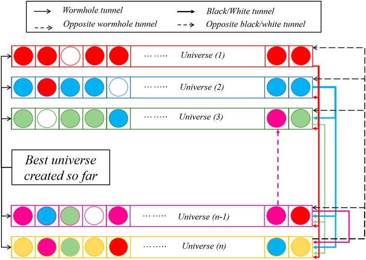
FIGURE 1. Conceptual model of the proposed OBL-MVO algorithm $r_2\left(NI\left(U_{best}\right)>NI\left(U_1\right)>NI\left(U_2\right)\cdots \cdots >NI\left(U_n\right)\right)$.

The following section introduces the initialization of the positive universe and the negative universe, the anti-black hole mechanism, the anti-white hole mechanism, and the anti-wormhole mechanism.

Anti-multiverse establishment: In order to solve the situation of the optimal value of the MVO algorithm often being too far from the real value in the early stage, the global search ability and convergence speed of the algorithm are improved. From the establishment stage of the multiverse population, the universe is divided into a positive universe and negative universe (the number of populations is consistent with the original MVO algorithm), and the positive universe is established by Eqs 6–9:

$U=\left[\begin{array}{cccc}{x}_1^1& x_1^2& \cdots & x_1^d\\ x_2^1& x_2^2& \cdots & x_2^d\\ ⋮& ⋮& ⋮& ⋮\\ x_{n/2}^1& x_{n/2}^2& \cdots & x_{n/2}^d\end{array}\right],(6)$

${x^{\prime }}_i^j={ub}_j-x_i^j+{ub}_j,(7)$

$U^{\prime }=\left[\begin{array}{cccc}{x^{\prime }}_1^1& {x^{\prime }}_1^2& \cdots & {x^{\prime }}_1^d\\ {x^{\prime }}_2^1& {x^{\prime }}_2^2& \cdots & {x^{\prime }}_2^d\\ ⋮& ⋮& ⋮& ⋮\\ {x^{\prime }}_{n/2}^1& {x^{\prime }}_{n/2}^2& \cdots & {x^{\prime }}_{n/2}^d\end{array}\right],(8)$

$U_{all}=\left[\begin{array}{cc}U& U^{\prime }\end{array}\right].(9)$

Here, $x_i^{\prime }$ is the corresponding negative universe in the positive universe $x_i$ and ${x^{\prime }}_i^j$ is the anti-object of the corresponding object in the negative universe.

Anti-black hole mechanism and anti-white hole mechanism: The material exchange mechanism between black holes and white holes is the exploration of the search space by MVO, but there are problems of the local search accuracy being too high and global search ability being insufficient. Therefore, the global search ability and overall stability of the algorithm are increased by setting the reverse black hole and reverse white hole mechanisms. The reverse black hole and reverse white hole mechanisms include random black hole and white hole stage and reverse object propagation stage. Both stages are controlled by a convergence factor $\lambda$ that decreases linearly with the number of iterations to control the probability of occurrence. The random black hole and white hole stages are shown in Eq. 11, and the reverse object propagation stage is shown in Eq. 12:

$\lambda =1-\frac{l}{L},(10)$

$x_i^j=\left\{\begin{array}{cc}{x}_k^j,& r_7<\lambda ,\\ x_i^j,& r_7\ge \lambda ,\end{array}\right.(11)$

$x_i^j=\left\{\begin{array}{cc}\left\{\begin{array}{cc}{x}_k^j,& r_5<0.5,\\ x_i^j,& r_5\le 0.5,\end{array}\right.& r_6<\lambda ,\\ x_i^j,& r_6\ge \lambda ,\end{array}\right.(12)$

where $\lambda$ is a convergence factor that decreases linearly with the number of iterations. $r_5$ and $r_6$ are random numbers in the range [0, 1].

The anti-wormhole mechanism: The anti-wormhole mechanism differs from the wormhole mechanism, where the anti-wormhole mechanism improves the global search by searching backward from the universe with the lowest expansion rate. To prevent this mechanism from affecting convergence, internal objects are, therefore, only stimulated to move toward the current worst universe if it is determined that the anti-wormhole mechanism is favorable to the increase in the universe’s expansion rate.

$x_i^j{\left(l+1\right)}_{opposite}=\left\{\begin{array}{cc}\left\{\begin{array}{cc}{x}_i^j+X_j^{\prime }\times TDR\times \left(\left({ub}_j-{lb}_j\right)\times r_4+{lb}_j\right),& r_3<0.5,\\ x_i^j+X_j^{\prime }\times TDR\times \left(\left({ub}_j-{lb}_j\right)\times r_4+{lb}_j\right),& r_3\ge 0.5,\end{array}\right.& r_2<WEP\&r_6<\lambda ,\\ x_i^j,& r_2\ge WEP\parallel r_6<\lambda ,\end{array}\right.(13)$

$x_i^j\left(l+1\right)=\left\{\begin{array}{cc}{x}_i^j{\left(l+1\right)}_{opposite},& NI\left(x_i^j{\left(l+1\right)}_{opposite}\right)>NI\left(x_i^j\left(l\right)\right),\\ x_i^j\left(l\right),& NI\left(x_i^j{\left(l+1\right)}_{opposite}\right)\le NI\left(x_i^j\left(l\right)\right),\end{array}\right.(14)$

where $X_j^{\prime }$ denotes the $j$ object of the current worst universe. $x_i^j{\left(l+1\right)}_{opposite}$ denotes the result of the calculation based on the reverse wormhole mechanism, $x_i^j\left(l+1\right)$ is the $j$ variable of the $i$ universe where the number of iterations is $l+1$, and $x_i^j\left(l\right)$ is the $j$ variable of the $i$ universe before the reverse wormhole mechanism in the $l$ iteration.

2.3 Adaptive ensemble learning by opposite multiverse optimizer

The idea of ensemble learning is that even if one base learner makes a wrong prediction, other base learners can correct the error, which aims to integrate multiple base learners to improve the accuracy of prediction. The main process is to first train multiple base learners by certain rules, then combine them using an integration strategy, and finally predict the result by comprehensive judgment of all base learners. Currently, ensemble learning has been successfully applied in pattern recognition, text classification, numerical prediction (Wang et al., 2011), and other fields.

The current integration strategy can be broadly divided into two categories: one is the sequential generation of base classifiers, with strong dependencies between individual learners, represented by AdaBoost (Ying et al., 2013), and the other is the parallelized integration method, which can generate base classifiers simultaneously, without strong dependencies between individuals, represented by Bagging (Dudoit and Fridlyand, 2003).

As unconventional reservoir data are collected from different reservoirs and have different reservoir data characteristics, this study improves the accuracy of the model by accommodating as many base learners as possible into a parallelized integration method to suit the different reservoir data characteristics. However, accommodating more models can lead to overfitting (Džeroski and Ženko, 2004). Therefore, the K-fold cross-validation method and opposition-based learning are introduced to avoid overfitting.

In this study, the search for the best weights of base learners is considered an optimization problem, and the OBL-MVO algorithm is used to solve the optimization problem. The integration strategy of AIL-OMO is to divide the original dataset into several sub-datasets which are fed into each base learner in layer 1. In layer 1, each base learner outputs its own prediction results as meta features. The meta features are then used as an input to layer 2, where the OBL-MVO is used to search for the best weights of base learners.

The integration strategy used in this study is shown in Figure 2.

FIGURE 2

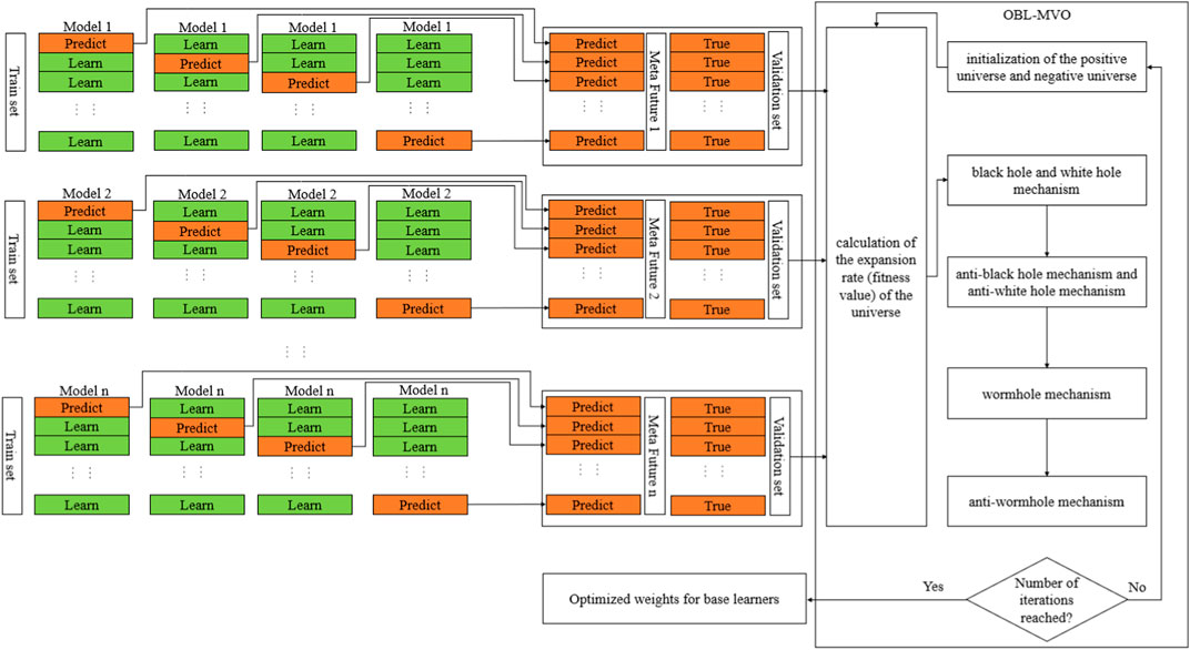
FIGURE 2. Integration strategy of AIL-OMO.

In order to fully exploit the individual strengths of each model, the probabilities of each reservoir predicted by each model are used as an input to train the ensemble learning model. In order to improve the accuracy and generalize the ability of the models completed by integration learning, the aforementioned OBL-MVO algorithm is introduced to reasonably optimize the integration learning process and search for the best weight of base learners.

The main contributions of this study are as follows:

(1) Collection of data and work on data collation and labeling.

(2) Proposed an algorithm OBL-MVO to optimize integration learning.

(3) Proposed an ensemble learning model AIL-OMO for the reservoir fluid classification task.

3 Experiments and results

To validate the effectiveness of our proposed method, we conducted experiments on the dataset. The following sections provide details on the model implementation, dataset processing, and final comparison results. The Flowchart of the AIL-OMO is shown in the Figure 3.

FIGURE 3

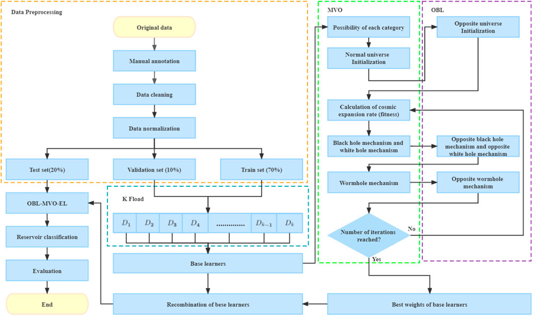
FIGURE 3. Flowchart of the AIL-OMO.

3.1 Data source and pretreatment

In this section, the data used in this paper and the preprocessing of the data are introduced. In order to build a reservoir classification model that can adapt to various unconventional features, 12,379 pieces of reservoir fluid property data from eight different wells were used for training the model. The data contain six categories of labels: dry layer, poor oil layer, water layer, oil-bearing water layer, oil–water layer, and oil layer. The data include AC (sonic interval transit time), CNL (compensated neutron logging), DEN (compensated density), GR (natural gamma ray), SP (spontaneous potential), CAL (caliper logging), and R045 (0.45 m potential resistivity). Figure 4 shows the degree of correlation between variables in reservoir fluid property data (excluding the oil field name). After obtaining the collected data, the annotation work of the dataset was carried out by analyzing the logging curves as the training data for the model.

FIGURE 4

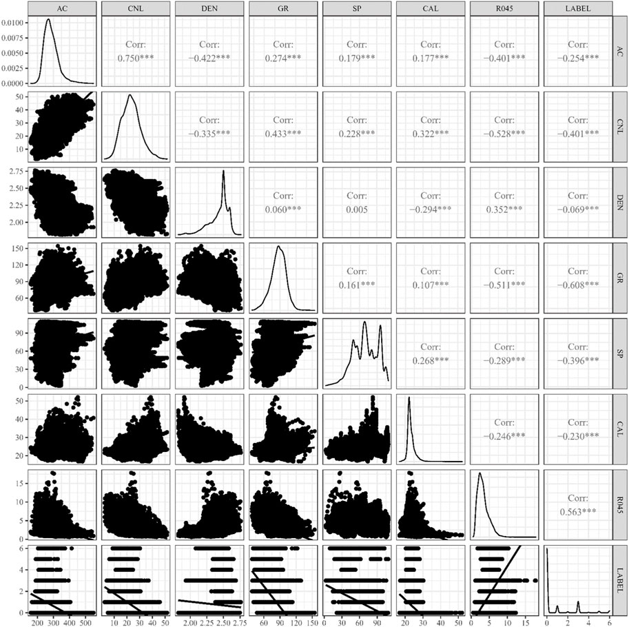
FIGURE 4. Correlation scatterplot matrix of the original dataset.

In the data preprocessing stage, this study mainly operates on the following issues:

(1) Rejection operations for data that are missing or do not conform to common sense.

(2) For labels with labeled data, one-hot coding is used for processing. Category labels from 1 to 6 represent the dry layer, poor oil layer, water layer, oil-bearing water layer, oil–water layer, and oil layer.

(3) Data normalization of the data is used as an input to the model.

3.2 Implementation details

In this section, OBL-MVO is used to solve the optimization problem to build adaptive ensemble learning classifiers for reservoir fluid property prediction. Since the dataset of unconventional reservoirs contains various unconventional reservoir features, each base learner is differently adapted to the unconventional reservoir features. Therefore, the weight searching problem in the integration strategy is abstracted as an optimization problem to obtain and integrate a model with generalization performance on all unconventional reservoir features in the dataset. The OBL-MVO algorithm is used to optimize the weights of the base learners based on the K-fold cross-validation test set to build the AIL-OMO to avoid the overfitting of partial features for unconventional reservoirs. In this optimization problem, to avoid overfitting of the local features of unconventional reservoirs, the accuracy of the validation set in K-fold cross-validation of each base learner for each unconventional reservoir feature is obtained from the validation set in K-fold cross-validation. In this case, the weights of the base learners are encoded into the individual dimensional attributes of the population, as shown in Eq. 15. The degree of learning of each model in each unconventional reservoir feature is involved in the calculation of the adaptation value of the optimization algorithm, as shown in Eq. 16.

$X_i=\left[\begin{array}{cccc}{x}_i^1& x_i^2& \cdots & x_i^d\end{array}\right],x_i^j\mathrm{ϵ}\left[\mathrm{0,1}\right]\left(1\le j\le d\right),(15)$

$fitness=1-\frac{{\displaystyle \sum _{i=1}^{ts}}\left[\max \left({\displaystyle \sum _{j=1}^{\mathit{dim}}}{x}_i^j\bullet x_i^j\right)-y_{ture}^i\right]}{ts},(16)$

where $X_i$ represents the individual $i$; $d$ is the dimension vector of $X_i$; $x_i^j$ is the $jth$ dimension value of the individual $i$, representing the weight of the $jth$ model; $y_i^j$ is the classification possibility of the $jth$ model in the test set of K-fold cross-validation; $y_{ture}^i$ is the true classification of the $ith$ sample; $ts$ is the number of samples in the full test set in K-fold cross-validation; and $fitness$ is the fitness function set by this study.

In order to show the performance of OBL-MVO on this dataset, OBL-MVO is compared with the other swarm intelligence heuristic algorithms, including whale optimization algorithm (WOA), gray wolf optimization (GWO), and MVO.

Among them, the parameter settings of each swarm intelligence heuristic algorithm are shown in Table 1.

TABLE 1

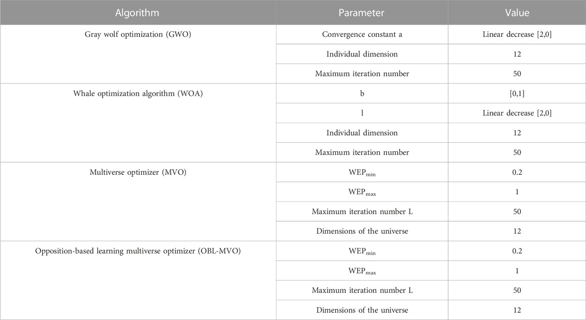
TABLE 1. Parameter size setting of the heuristic algorithms.

In order to compare the four intelligent optimization algorithms, it is necessary to compare the fitness value curves of their optimization results. Since the population size of different algorithms affects the convergence of the fitness curve, in order to balance the effect of the population size of each algorithms on the fitness value, the population size for each algorithm is set to 20, 50, 100, and 200. The fitness curve results of GWO, WOA, MVO, and OBL-MVO are shown in Figure 5.

FIGURE 5

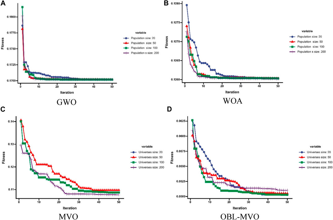
FIGURE 5. Fitness curve of OBL-PO and other algorithms. (A)GWO, (B) WOA, (C) MVO, and (D) OBL-MVO.

Figure 5 shows that OBL-MVO has a faster convergence rate than MVO, WOA, and GWO (the number of iterations required for the fitness function to converge and stabilize is the least); OBL-MVO shows a better convergence fitness value than MVO, WOA, and GWO, indicating that OBL-MVO has a better optimization effect than MVO, WOA, and GWO on the dataset. The corresponding weights of base learners optimized by OBL-MVO adaptive optimization are shown in Table 2.

TABLE 2

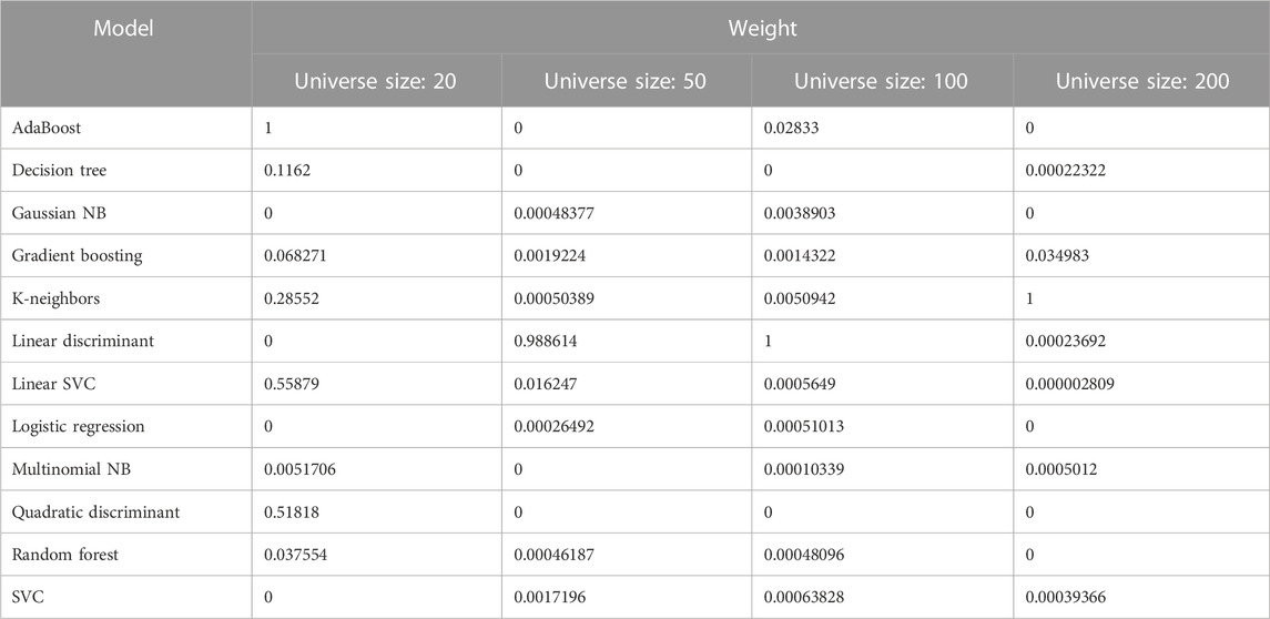
TABLE 2. Weight of the base learners adapted by OBL-MVO.

3.3 Reservoir fluid property prediction

In this section, the predicted results of the AIL-OMO model and evaluation of its performance are presented. The AIL-OMO model was trained using the training dataset and evaluated on the test set. This paper adopts the accuracy rate as the evaluation metric, which is widely used in reservoir classification, lithology identification, and reservoir fluid identification (Moffatt and Williams, 1998; Al-Anazi and Gates, 2010; Boyd et al., 2013; Onwuchekwa, 2018).

Figure 6 depicts the results of using seven machine learning algorithms to predict the reservoir fluid, including the AIL-OMO model proposed in this paper. The accuracy of the AIL-OMO model surpasses that of the other six models, achieving an accuracy rate of 92.75%, followed by the SVC and linear SVC models in well 1. Figure 7 presents the reservoir fluid prediction results of the seven machine learning models in well 2. The accuracy rates from high to low are given as follows: AIL-OMO (81.93%), logistic regression (70.37%), linear SVC (69.30%), linear discriminant analysis (69.26%), KNN (69.11%), AdaBoost (66.45%), and SVC (64.37%). Figure 8 shows the reservoir fluid prediction results of the seven machine learning models in well 3. Among the prediction results of each model, the accuracy rate of the AIL-OMO model is better than that of the other models, with an accuracy rate of 88.72%, followed by SVC with an accuracy rate of 83.03%. The worst model is AdaBoost, with an accuracy rate of only 65.57%. From the experimental results, it can be interpreted that integrating multiple weak learners into one strong learner using the OBL-MVO algorithm leads to a significant improvement in the prediction accuracy of the original model. Therefore, the proposed AIL-OMO model has high accuracy and is more conducive to the prediction of reservoir fluid.

FIGURE 6

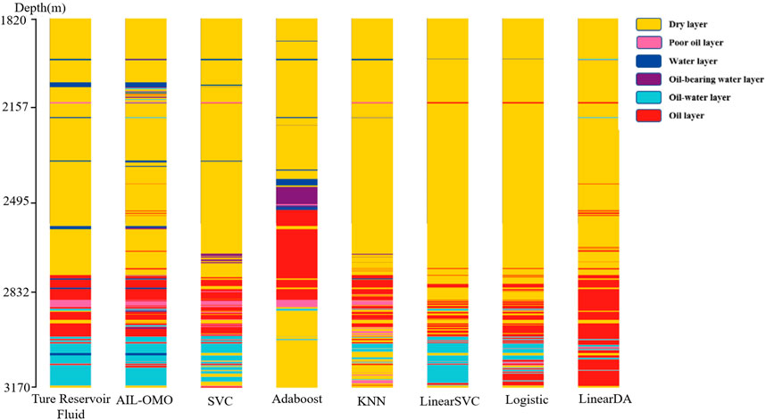
FIGURE 6. Comparison chart of the real reservoir fluid and predicted reservoir fluid in well 1.

FIGURE 7

FIGURE 7. Comparison chart of the real reservoir fluid and predicted reservoir fluid in well 2.

FIGURE 8

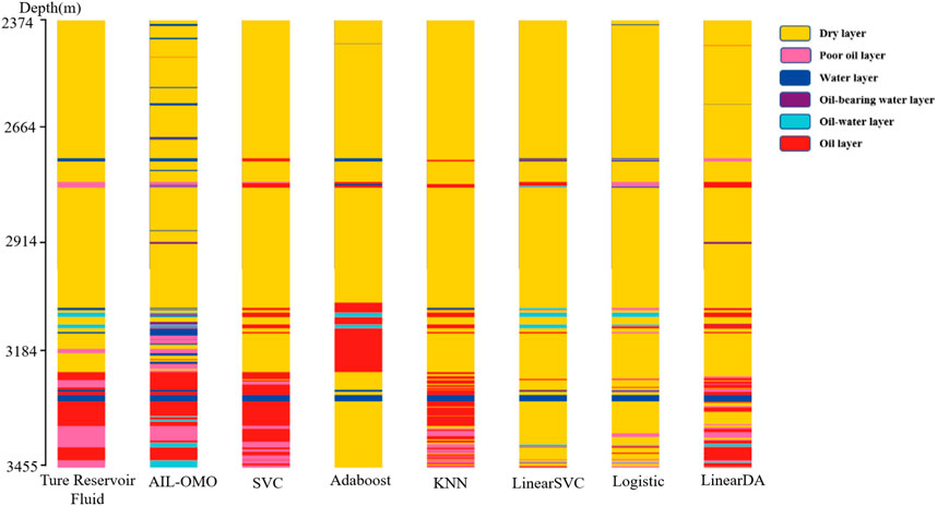
FIGURE 8. Comparison chart of the real reservoir fluid and predicted reservoir fluid in well 3.

Figure 9 shows the change in the classification accuracy of the AIL-OMO model with different party sizes.

FIGURE 9

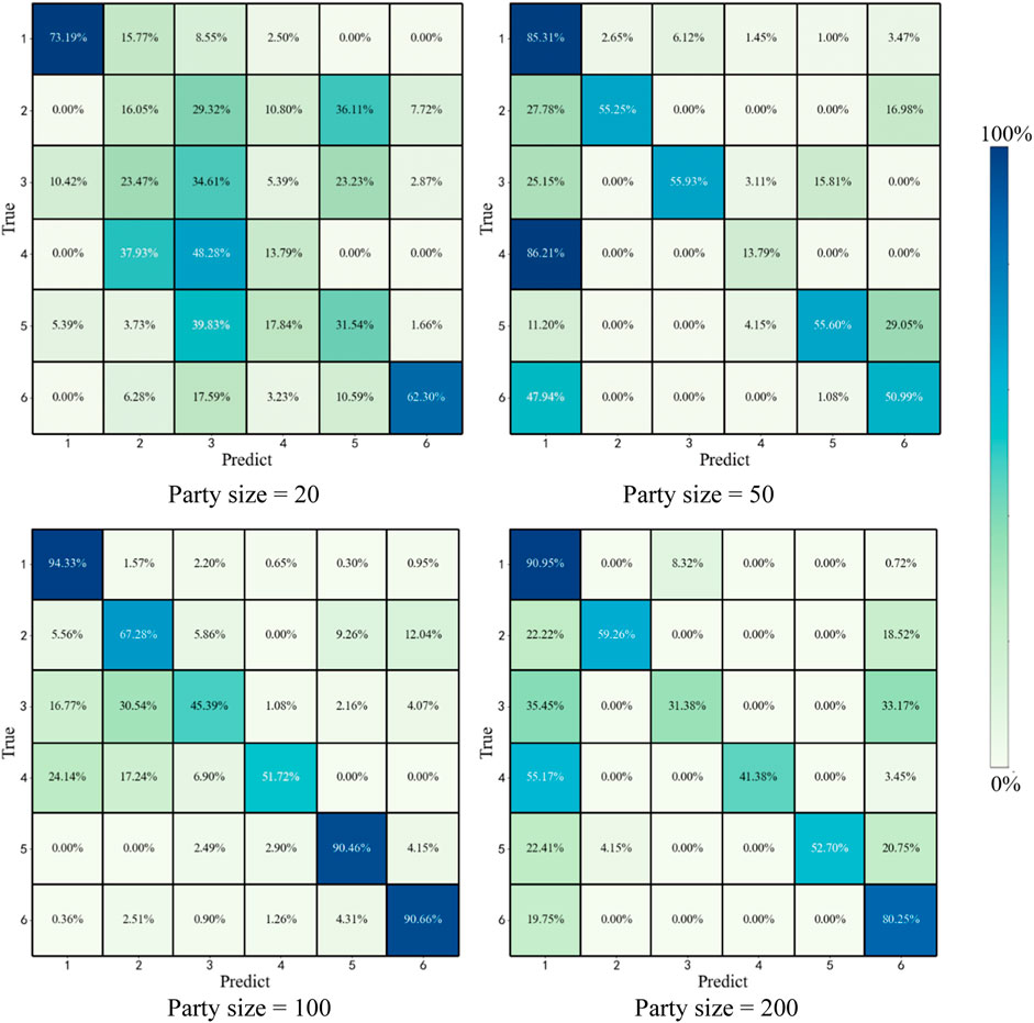
FIGURE 9. Reservoir fluid property prediction by AIL-OMO (classification label: dry layer (1), poor oil layer (2), water layer (3), oil-bearing water layer (4), oil–water layer (5), and oil layer (6)).

Figure 9 shows the classification accuracy of different reservoir fluids by AIL-OMO. Each value in the figure represents the ratio of the number of reservoir fluids identified by AIL-OMO to the actual number of reservoir fluids in the dataset. Figure 6 shows that the results of AIL-OMO exhibit slight fluctuations under different party sizes. The classification accuracy for the poor oil layer, water layer, and oil-bearing water layer is relatively low. This can be attributed to the smaller percentage of poor reservoirs, water layers, and oil-bearing water layers in the dataset.

Table 3 presents the comparison results of the accuracy of AIL-OMO and the other six machine learning models. Among them, AIL-OMO with a party size of 100 achieves the highest accuracy of 85%. This model demonstrates the fewest classification errors for each reservoir. However, when the party size is increased to 200, the accuracy of AIL-OMO decreases to 78%. This decrease in accuracy can be attributed to the party size being too large, causing overfitting of the model to the data.

TABLE 3

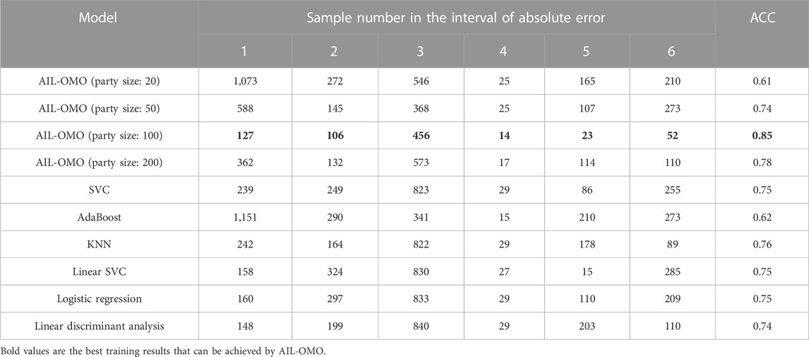
TABLE 3. Specific results of predicting permeability.

4 Discussion

Considering the characteristics of ensemble learning, the MVO algorithm may promote the overfitting learning phenomenon in the fluid category with small sample data. Therefore, the more models the AIL-OMO integrates, the more the corresponding training data samples should be, so that MVO can achieve the optimization effect of ensemble learning.

For each model, the identification of oil-bearing water layer and water layer are not accurate enough, which may be due to the classification confusion caused by noise interference in the logging curves of the water layer in unconventional reservoirs. In the future, we aim to decrease the number of base models to improve the operational speed and enhance our model’s performance by collecting data from various reservoir types for testing.

5 Conclusion

This study focuses on logging data for unconventional reservoirs, which exhibit unconventional characteristics and data imbalance. To address these challenges, this paper proposes a new model that combines 12 base learners using the multiverse optimizer. The AIL-OMO model combines multiple weak learners into one strong learner. The advantage of our ensemble learning lies in its ability to ensure the diversity of weak classifiers, resulting in better prediction results than those obtained by other single learner models. Compared to other widely used models, the new ensemble learning model proposed in this paper achieves high accuracy on classifying dry layers, oil–water layers, and oil layers, with accuracy rates of 94.33%, 90.46%, and 90.66%, respectively. This indicates that the proposed model exhibits the highest accuracy and better generalization for fluid identification in unconventional oil reservoirs.

Data availability statement

The raw data supporting the conclusion of this article will be made available by the authors, without undue reservation.

Author contributions

YZ: writing—original draft and resources; XZ: methodology and supervision; YS: visualization and investigation; AG: data curation and conceptualization; ML: validation. All authors contributed to the article and approved the submitted version.

Funding

This work was financially supported by the Major Scientific and Technological Projects of CNPC under Grant ZD2019-183-004.

Conflict of interest

The authors declare that the research was conducted in the absence of any commercial or financial relationships that could be construed as a potential conflict of interest.

Publisher’s note

All claims expressed in this article are solely those of the authors and do not necessarily represent those of their affiliated organizations, or those of the publisher, the editors, and the reviewers. Any product that may be evaluated in this article, or claim that may be made by its manufacturer, is not guaranteed or endorsed by the publisher.

References

Al-Anazi, A., and Gates, I. D. (2010). A support vector machine algorithm to classify lithofacies and model permeability in heterogeneous reservoirs. Eng. Geol. 114, 267–277. doi:10.1016/j.enggeo.2010.05.005

CrossRef Full Text | Google Scholar

Baarimah, S. O., Al-Aidroos, N. M., and Ba-Jaalah, K. S. (2019). Using chemical composition of crude oil and artificial intelligence techniques to predict the reservoir fluid properties. Int. Conf. Intell. Comput. Eng. (ICOICE), 1–5. doi:10.1109/ICOICE48418.2019.9035135

CrossRef Full Text | Google Scholar

Bestagini, P., Lipari, V., and Tubaro, S. (2017). A machine learning approach to facies classification using well logs Seg technical program expanded abstracts 2017. Houston, Texas, United States: Society of Exploration Geophysicists, 2137–2142.

Google Scholar

Boyd, K., Eng, K. H., and Page, C. D. “Area under the precision-recall curve: Point estimates and confidence intervals,” in Proceedings of the Joint European conference on machine learning and knowledge discovery in databases, Prague, Czech Republic, September 2013 (Springer), 451–466.

Google Scholar

Dao, T., Yu, J., Nguyen, T., and Ngo, T. (2020). A hybrid improved MVO and FNN for identifying collected data failure in cluster heads in WSN. IEEE Access 8, 124311–124322. doi:10.1109/access.2020.3005247

CrossRef Full Text | Google Scholar

Das, B., and Chatterjee, R. (2018). Well log data analysis for lithology and fluid identification in Krishna-Godavari Basin, India. Arabian J. Geosciences 11, 231–312. doi:10.1007/s12517-018-3587-2

CrossRef Full Text | Google Scholar

Dudoit, S., and Fridlyand, J. (2003). Bagging to improve the accuracy of a clustering procedure. Bioinformatics 19, 1090–1099. doi:10.1093/bioinformatics/btg038

PubMed Abstract | CrossRef Full Text | Google Scholar

Džeroski, S., and Ženko, B. (2004). Is combining classifiers with stacking better than selecting the best one? Mach. Learn 54, 255–273. doi:10.1023/b:mach.0000015881.36452.6e

CrossRef Full Text | Google Scholar

Ewees, A. A., Abd Elaziz, M., and Houssein, E. H. (2018). Improved grasshopper optimization algorithm using opposition-based learning. Expert Syst. Appl. 112, 156–172. doi:10.1016/j.eswa.2018.06.023

CrossRef Full Text | Google Scholar

Guerreiro, J. N. C., Barbosa, H. J. C., Garcia, E. L. M., Loula, A. F. D., and Malta, S. M. C. (1998). Identification of reservoir heterogeneities using tracer breakthrough profiles and genetic algorithms. SPE Reserv. Eval. Eng. 1, 218–223. doi:10.2118/39066-pa

CrossRef Full Text | Google Scholar

Gupta, S., and Deep, K. (2019). A hybrid self-adaptive sine cosine algorithm with opposition based learning. Expert Syst. Appl. 119, 210–230. doi:10.1016/j.eswa.2018.10.050

CrossRef Full Text | Google Scholar

Hassan, H. A., and Zellagui, M. “MVO algorithm for optimal simultaneous integration of DG and DSTATCOM in standard radial distribution systems based on technical-economic indices,” in Proceedings of the 2019 21st International Middle East Power Systems Conference (MEPCON), Cairo, Egypt, December 2019, 277–282.

Google Scholar

He, M., Gu, H., and Wan, H. (2020). Log interpretation for lithology and fluid identification using deep neural network combined with MAHAKIL in a tight sandstone reservoir. J. Pet. Sci. Eng. 194, 107498. doi:10.1016/j.petrol.2020.107498

CrossRef Full Text | Google Scholar

Jain, G., Yadav, G., Prakash, D., Shukla, A., and Tiwari, R. (2019). MVO-based path planning scheme with coordination of UAVs in 3-D environment. J. Comput. Sci. 37, 101016. doi:10.1016/j.jocs.2019.07.003

CrossRef Full Text | Google Scholar

Luo, G., Xiao, L., Liao, G., Luo, S., Shao, R., Zhou, J., et al. (2022). Multi-level reservoir identification with logs based on machine learning SPWLA 63rd annual logging symposium. Richardson, TX, United States: OnePetro.

Google Scholar

Mirjalili, S., Mirjalili, S. M., and Hatamlou, A. (2016). Multi-verse optimizer: A nature-inspired algorithm for global optimization. Neural Comput. Appl. 27, 495–513. doi:10.1007/s00521-015-1870-7

CrossRef Full Text | Google Scholar

Moffatt, B. J., and Williams, J. M. (1998). Identifying and meeting the key needs for reservoir fluid properties A multi-disciplinary approach spe annual technical conference and exhibition. Richardson, TX, United States: OnePetro.

Google Scholar

Onwuchekwa, C. (2018). Application of machine learning ideas to reservoir fluid properties estimation SPE Nigeria Annual International Conference and Exhibition. Richardson, TX, United States: OnePetro.

Google Scholar

Sun, J., Li, Q., Chen, M., Ren, L., Huang, G., Li, C., et al. (2019). Optimization of models for a rapid identification of lithology while drilling - a win-win strategy based on machine learning. J. Pet. Sci. Eng. 176, 321–341. doi:10.1016/j.petrol.2019.01.006

CrossRef Full Text | Google Scholar

Tizhoosh, H. R. “Opposition-based learning: A new scheme for machine intelligence,” in Proceedings of the International conference on computational intelligence for modelling, control and automation and international conference on intelligent agents, web technologies and internet commerce (CIMCA-IAWTIC'06), Vienna, Austria, November, 2005, 695–701.

Google Scholar

Tohidi-Hosseini, S., Hajirezaie, S., Hashemi-Doulatabadi, M., Hemmati-Sarapardeh, A., and Mohammadi, A. H. (2016). Toward prediction of petroleum reservoir fluids properties: A rigorous model for estimation of solution gas-oil ratio. J. Nat. Gas. Sci. Eng. 29, 506–516. doi:10.1016/j.jngse.2016.01.010

CrossRef Full Text | Google Scholar

Tubishat, M., Idris, N., Shuib, L., Abushariah, M. A., and Mirjalili, S. (2020). Improved Salp Swarm Algorithm based on opposition based learning and novel local search algorithm for feature selection. Expert Syst. Appl. 145, 113122. doi:10.1016/j.eswa.2019.113122

CrossRef Full Text | Google Scholar

Vivek, K., Deepak, M., Mohit, J., Asha, R., and Vijander, S. (2018). Development of multi-verse optimizer (mvo) for labview intelligent communication, control and devices. Berlin, Germany: Springer, 731–739.

CrossRef Full Text | Google Scholar

Wang, H., Wu, Z., Rahnamayan, S., Liu, Y., and Ventresca, M. (2011). Enhancing particle swarm optimization using generalized opposition-based learning. Inf. Sci. 181, 4699–4714. doi:10.1016/j.ins.2011.03.016

CrossRef Full Text | Google Scholar

Wang, P., Chen, X., Wang, B., Li, J., and Dai, H. (2020). An improved method for lithology identification based on a hidden Markov model and random forests. Geophysics 85, IM27–IM36. doi:10.1190/geo2020-0108.1

CrossRef Full Text | Google Scholar

Yang, H., Pan, H., Ma, H., Konaté, A. A., Yao, J., and Guo, B. (2016). Performance of the synergetic wavelet transform and modified K-means clustering in lithology classification using nuclear log. J. Pet. Sci. Eng. 144, 1–9. doi:10.1016/j.petrol.2016.02.031

CrossRef Full Text | Google Scholar

Ying, C., Qi-Guang, M., Jia-Chen, L., and Lin, G. (2013). Advance and prospects of AdaBoost algorithm. Acta Autom. Sin. 39, 745–758. doi:10.1016/s1874-1029(13)60052-x

CrossRef Full Text | Google Scholar

Zhang, T., and Sun, S. (2021). Thermodynamics-informed neural network (TINN) for phase equilibrium calculations considering capillary pressure. Energies 14, 7724. doi:10.3390/en14227724

CrossRef Full Text | Google Scholar

Zhou, J., Huang, S., and Qiu, Y. (2022). Optimization of random forest through the use of MVO, GWO and MFO in evaluating the stability of underground entry-type excavations. Tunn. Undergr. Space Technol. 124, 104494. doi:10.1016/j.tust.2022.104494

CrossRef Full Text | Google Scholar