 Ye Fan
 Wenbao Hu3*
 Ji Tang
 Qing Ye
95% of researchers rate our articles as excellent or good
Learn more about the work of our research integrity team to safeguard the quality of each article we publish.
Find out more
ORIGINAL RESEARCH article
Front. Earth Sci. , 15 May 2023
Sec. Solid Earth Geophysics
Volume 11 - 2023 | https://doi.org/10.3389/feart.2023.1110056
This article is part of the Research Topic From Preparation to Faulting: Multidisciplinary Investigations on Earthquake Processes, volume II View all 16 articles
The main components of seismo-electromagnetic research are the deep underground electromagnetic seismogenic environment, electromagnetic field changes at different stages of the seismogenic process, and the physical mechanism and change rules of electromagnetic properties of the earth’s interior. Traditional electric and magnetic methods mainly analyze the single field change of the geoelectric field, geomagnetic field, or resistivity at frequencies less than 1 Hz. These do not include the extremely low-frequency band that is sensitive to seismic events, so it is difficult to obtain the characteristics of time-spatial variations and propagation characteristics precursors. In comparison, magnetotelluric stations observe magnetotelluric fields containing seismogenic-induced electromagnetic disturbances, and the observation frequency band is wide. In this paper, the three-dimensional numerical simulation method is used to calculate the magnetotelluric apparent resistivity anomaly generated by resistivity changes in the seismogenic zone, and the forward algorithm of arbitrarily orientated dipole source in layered earth is used to simulate the response of low-frequency pre-earthquake electromagnetic radiation. The magnetotelluric response including seismogenic resistivity anomaly and pre-earthquake electromagnetic radiation is obtained using the field component composition method. The frequency characteristics and spatial distribution characteristics of apparent resistivity anomalies are systematically analyzed, and the results are of important significance for the observation, data processing, and identification and analysis of seismic electromagnetic anomalies in different seismogenic processes.
Physical quantities that can be related to electromagnetic anomalies in the earthquake developing process mainly include earth resistivity, geomagnetic field, geoelectric field, electromagnetic induction field, and electromagnetic radiation (Zhao et al., 2022). In a deep underground electromagnetic seismogenic environment, changes in the electromagnetic field in the seismogenic process, and the physical mechanism and change characteristics of electromagnetic properties of the earth’s interior are the main contents of seismo-electromagnetic research (Mao, 1986). Since the 1960s, there has been systematic research and observations of seismogenic electromagnetic phenomena in China. Observation stations have been successively set up in key earthquake risk areas for long-term observation of the geomagnetic field, geoelectric field, earth resistivity, magnetotelluric field, and electromagnetic radiation (Pan, 1998), recording a large number of electromagnetic precursors (Huang et al., 2017). In 2018, the experimental satellite Zhang Heng No.1 was launched for seismic electromagnetic monitoring in China; from this, a space-ground joint seismic electromagnetic monitoring system was established (Zhang et al., 2020). During this period, there has been theoretical and experimental research on the mechanism of earthquake electromagnetic precursors, distribution laws and propagation characteristics, correlation with seismic activity, and information extraction (Huang, 2002; Ma, 2002; Wang et al., 2005; Ding, 2009; Gao and Hu, 2010; Du, 2011; Huang et al., 2015; Ren et al., 2015; 2016; Zhou et al., 2017). These results confirm that the earthquake preparation process does cause electromagnetic anomalies, summarize the characteristics of temporal and spatial variations of seismic electromagnetic anomalies, and use numerical simulations to try to explain the generation mechanism and propagation selective phenomena of seismic electromagnetic signals and focus on numerical simulation research on the mechanism of earthquake electromagnetic co-seismic or post-earthquake attenuation (Gao et al., 2016; Hu et al., 2011), but there is still a lack of strong quantitative explanations for the identification characteristics of electromagnetic anomalies caused by the seismogenesis process.
The early earthquake precursor observation and data analysis methods in China have mainly used traditional electrical and magnetic methods to observe the changes in the geoelectric field, geomagnetic field (
The magnetotelluric sounding method based on the principle of electromagnetic induction has the characteristics of the wide frequency band and multi-component observation. Using magnetotelluric data from stations to identify and extract seismic electromagnetic anomaly information has the following advantages. 1) In data processing, the ratio of the mutually orthogonal electric and magnetic field is used to obtain the electromagnetic impedance of the earth and then the apparent resistivity and impedance phase information. This method can automatically eliminate the influence of magnetotelluric field changes of any frequency caused by the change of the earth’s electromagnetic environment. 2) Reliable regional background resistivity information at different depths can be obtained from long-term observations by the network, which is convenient for identifying and extracting resistivity anomalies. 3) The seismogenic resistivity anomaly has the characteristic of slow change over a long time, which is easy to distinguish from human activity and local spatial change. 4) Allows for better comprehensive analysis, the electromagnetic impedance anomaly of a magnetotelluric station not only includes the change in the resistivity of the underlying earth formation caused by stress change and fracture development in the adjacent areas but also includes the electromagnetic radiation information generated by pressure in the rock formation.
In many cases, the earth can be represented as a horizontally stratified medium with homogeneous and isotropic properties in each layer (Wait, 1951). In this paper, we introduce a three-dimensional low resistivity anomaly in the horizontally layered stratum model designed to simulate the change of the earth’s resistivity in the seismogenic zone, the electromagnetic impedance response in a large spatial range is calculated and its characteristics with frequency and space variation have been analyzed. Assuming that the electromagnetic radiation in the seismogenic region is equivalent to the vector electric dipole radiation source, the electromagnetic impedance response of electric dipole of different orientations is calculated and its characteristics of responses are analyzed. Finally, the dipole source response and magnetotelluric response are synthesized to simulate the observed response of the seismic electromagnetic anomaly by the magnetotelluric stations. From the perspective of 3D numerical simulation, we analyze the characteristics of an electromagnetic anomaly caused by earth resistivity changes and electromagnetic radiation during the pre-seismic period and propose methods to identify and extract different seismic electromagnetic anomalies. This will then provide theoretical support for extremely low-frequency electromagnetic observations used to monitor seismic electromagnetic anomalies.
This study concentrates on observations and processing of magnetotelluric data within a limited spatial area. Based on the one-dimensional (1D) horizontal layered stratum model, the 3D low resistivity anomaly is added to the high resistivity stratum to simulate the resistivity change caused by fracture development in the seismogenic area. The electromagnetic radiation generated by the sudden change of stress in the seismogenic center area before the earthquake is simulated with an inclined electric dipole source at depth.
The designed model structure is shown in Figure 1, where we use the x-y-z rectangular coordinate system with z = 0 at the ground surface and positive upward. Figure 1A shows the x-z resistivity section at y = 0 (shown by the dotted line in Figure 1B) of the horizontally layered model with a 3D low resistivity anomaly. Figure 1B is an x-y slice of resistivity at a depth of 10 km (as shown by the dotted line in Figure 1A), showing the plane structure of the 3D low resistivity anomaly. The top earth layer is a low-resistance cover layer with a thickness of
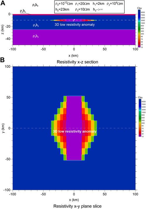
FIGURE 1. Horizontal layered and 3D low resistivity anomaly model using the x-y-z rectangular coordinate system with z=0 at the ground surface and positive upward (A) Is the resistivity x-z section, and (B) is the resistivity x-y plane slice at a depth of 10 km (z = −10 km).
Using 3D simulation software to calculate the magnetotelluric response of the horizontally layered model with the 3D low resistivity anomaly shown in Figure 1, we can obtain the apparent resistivity and phase information of the xy and yx components at the ground observation site. Figure 2 shows contour maps of the apparent resistivity of the two principal component elements with frequencies of 0.1, 0.05, and 0.01 Hz, respectively. Because the model structure is symmetrical, we only show quadrant 1 (with x=0–400 km and y=0–300 km) to investigate the distribution of electromagnetic impedance response. In Figure 2, white ladder lines are used to mark the corresponding positions and boundaries of the 3D low resistivity anomalous body at depth. Different color scales are used in contour maps because the amplitude of different frequency responses varies greatly.
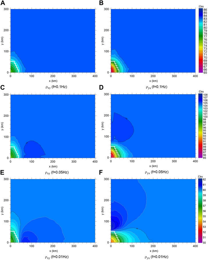
FIGURE 2. Contour maps of the spatial distribution of the apparent resistivity of the two principal components of the 3D model. (A,C,E) are the ρxy at the frequency of 0.1 Hz, 0.05 Hz, 0.01 Hz respectively; (B,D,F) are the ρyx at the frequency of 0.1 Hz, 0.05 Hz, 0.01 Hz respectively.
It can be seen from Figure 2 that 1) generally, the existence of a 3D low resistivity anomaly causes the apparent resistivity value above and near the 3D body to be significantly reduced. 2) The amplitude of the apparent resistivity anomaly is largest just above the 3D low resistivity body, and gradually decreases to background value with increasing distance from the boundary of the 3D low resistivity body, and the attenuation distance increases with decreasing frequency. For example, the distance of the
To quantitatively evaluate the sensitivity of the magnetotelluric response observed at the stations to the seismogenic resistivity anomaly, Figure 3 shows the ratio curve of the responses of the measuring sites at different offsets along the radial x) direction and axial y) direction of the 3D low resistivity anomaly to the responses of the 1D horizontal layered model of the corresponding measuring sites. The offsets of the measuring sites are 0, 10, 25, 50, 100, 200, and 400 km, respectively. The curve with a ratio of 1 represents the response of a 1D layered model, which is not disturbed by the 3D low resistivity anomaly. If the ratio is larger than 1, the apparent resistivity value increases, making this a positive anomaly. A ratio less than 1 indicates that the apparent resistivity value decreases, that is, a negative anomaly. Because the model contains the 3D low resistivity anomaly, the ratio curve should be dominated by negative anomalies, and how much the ratio deviates from 1 is the amplitude of the anomaly. The apparent resistivity ratio curve in Figure 3 shows that: 1) The influence of 3D low resistivity anomaly begins in the low-frequency band below 5 Hz. 2) In the frequency band of about 1∼5 Hz, the apparent resistivity ratio curve shows a positive abnormal overshoot, which is the intrinsic characteristic of the magnetotelluric response. The amplitude of overshoot is largest at zero offsets (up to about 7%) and decreases with an increasing offset; is approaching zero for x offset is greater than or equal to 50 km and while y offset is greater than or equal to 100 km. 3) Generally, in the low-frequency band below 1Hz, the ratio curve is dominated by negative anomalies, and the amplitude of the negative anomaly decreases with increasing offset distance. At the same offset distance, the amplitude of the
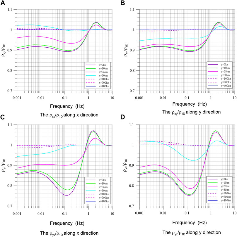
FIGURE 3. Apparent resistivity ratio of the three-dimensional model to one-dimensional layered model for measuring sites of different offsets along x- and y-direction. (A) and (B) are the ρxy/ρ1D along x and y direction respectively; (C) and (D) are the ρxy/ρ1D along x and y direction respectively.
The apparent resistivity method is one of the earliest geophysical methods used for earthquake precursor monitoring in China. After years of observation and research, Qian et al. (1982) and Zhang et al. (1996) successively summarized the characteristics of the apparent resistivity anomaly before earthquakes: 1) The apparent resistivity anomaly before earthquakes can be divided into a long-trend anomaly and impending anomaly. 2) Before the earthquake, the apparent resistivity is mostly a decreasing anomaly, though some increasing changes have also been observed. The anomaly amplitude decreases with increasing epicenter distance. 3) Before the earthquake, the long trend anomaly extends outward from the epicenter area, extending out to 150 km. 4) The anomalies are directional. 5) The standard deviation of the monthly average value of the active source apparent resistivity observation method should be less than 0.5%. If the apparent resistivity has a continuous multipoint trend change and the amplitude exceeds 3 times the standard error, it can be identified as the anomaly. Our simulation results described above provide a theoretical basis for the characteristics of the apparent resistivity anomaly in the seismogenic area summarized by precursors and verify the identification rule of the resistivity anomaly.
The electromagnetic responses of the electric dipole source in the horizontally layered earth are calculated using the algorithm by Hu et al. (2023), and the propagation characteristics of the electric dipole source radiation field in earth and its influence on ground observations have been investigated. For comparative studies, the responses of a horizontal and an incline electric dipole in uniform earth and horizontally layered earth are calculated and analyzed respectively.
An x-direction horizontal electric dipole source (azimuth angle
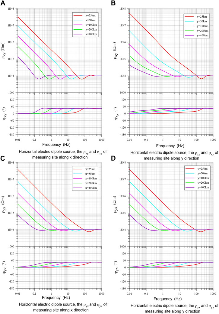
FIGURE 4. Apparent resistivity and phase response of a horizontal dipole source in a homogeneous earth for measuring sites of different offsets along x- and y-direction. (A) and (B) are the ρxy and φxy of measuring sites along x and y direction respectively; (C) and (D) are the ρyx and φyx of measuring sites along x and y direction respectively.
For the field responses of horizontal electric dipole source, the area with an offset greater than
Since the impedance response of the vertical electric dipole source does not have plane wave characteristics as defined by the field responses observed on the ground, it is not presented here. For the field of an inclined dipole source in the earth, the field responses observed on the ground will be affected by the vertical source field, which is much different from the field of a simple horizontal dipole source. Figure 5 shows the curves of apparent resistivity and phase excited by a 30° inclined electric dipole source at 10 km deep from the earth’s surface, Figures 5A, B show
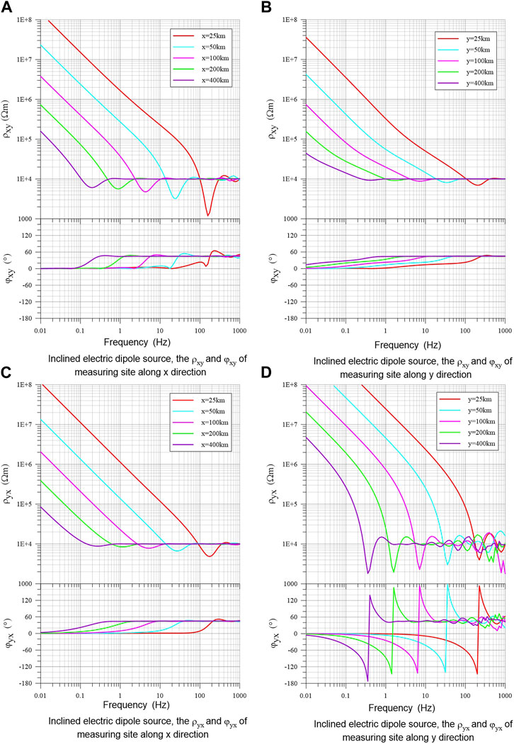
FIGURE 5. Apparent resistivity and phase response of an inclined dipole source in a homogeneous earth for measuring sites of different offsets along x- and y-direction. (A) and (B) are the ρxy and φxy of measuring sites along x and y direction respectively; (C) and (D) are the ρyx and φyx of measuring sites along x and y direction respectively.
The frequency characteristics of apparent resistivity and phase response of electric dipole in layered earth medium may become complex due to the difference in sensitivity of different frequencies to different depths. Figure 6 shows the apparent resistivity and phase curves of the horizontal electric dipole source with different offsets along the x - and y-directions in the three-layer earth model. Note that the impedance phases of the two principal component elements have been corrected to the 45
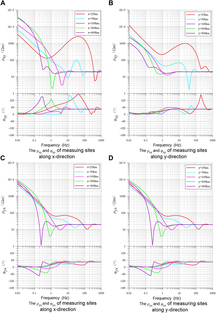
FIGURE 6. Apparent resistivity and phase curves of the horizontal electric dipole source in a three-layer earth model for measuring sites of different offsets along x- and y-direction. (A) and (B) are the ρxy and φxy of measuring sites along x and y direction respectively; (C) and (D) are the ρyx and φyx of measuring sites along x and y direction respectively.
It can be seen from the above analyses that the electromagnetic response of the horizontal electric dipole source in the layered stratum can reflect the basic characteristics of the dipole source field. However, because of the influence of layered electrical structure, the frequency response curves in different directions, differing offsets, and polarization modes may have complex shapes and variation characteristics. To better understand the spatial distribution characteristics of the electromagnetic response of the horizontal electric dipole source, Figure 7 shows the x-y plane distribution of the apparent resistivity (
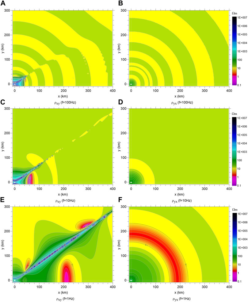
FIGURE 7. Contour plots in the x-y plane of apparent resistivity response of the x-direction horizontal electric dipole source in a three-layer earth. (A,C,E) are the ρxy at the frequency of 100 Hz, 10 Hz, 1 Hz respectively; (B,D,F) are the ρyx at the frequency of 100 Hz, 10 Hz, 1 Hz respectively.
Figure 8 shows the apparent resistivity and phase curves of the x-direction inclined (φ=30
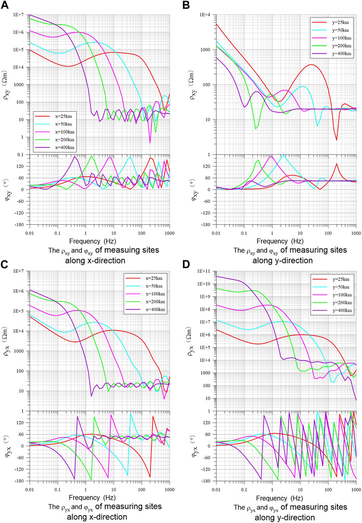
FIGURE 8. Apparent resistivity and phase curves of an inclined electric dipole source in three-layer earth for measuring sites of different offsets along x- and y-direction. (A) and (B) are the ρxy and φxy of measuring sites along x and y direction respectively; (C) and (D) are the ρyx and φyx of measuring sites along x and y direction respectively.
Figure 9 shows the plane distribution of the apparent resistivity of the inclined electric dipole source. To facilitate comparison, the same contour color scale as in Figure 7 is used. Compared with Figure 7, it can be seen that 1) the apparent resistivity of the inclined electric dipole source is much higher than that of the horizontal electric dipole source. 2) The area of near-source area apparent resistivity enhancement is much larger than the response of a simple horizontal dipole source. Taking

FIGURE 9. Contour plots in the x-y plane of apparent resistivity response of an inclined electric dipole source in a three-layer earth. (A,C,E) are the ρxy at the frequency of 100 Hz, 10 Hz, 1 Hz respectively; (B,D,F) are the ρyx at the frequency of 100 Hz, 10 Hz, 1 Hz respectively.
It can be seen from the apparent resistivity response of the tilt dipole source in the earth that when the radiation source contains vertical components, the amplitude and spatial range of the apparent resistivity anomaly in the near-field zone are greatly enhanced. Compared with the response of a simple horizontal electric dipole source, the amplitude of the high resistance anomaly is about 2–5 orders of magnitude higher. For the same offset, the frequency of the near-field zone anomaly increases by about an order of magnitude. The spatial range of near-field zone anomaly is about 3 times larger (taking 10 Hz response as an example). It can be seen that the vertical component of seismogenic electromagnetic radiation can greatly increase the detectability of anomalies.
The behaviors of the magnetotelluric response of the 3D anomaly of earth resistivity and the dipole response of buried electric dipole radiation source in the seismogenic zone have been presented in previous sections. We now discuss the magnetotelluric responses when the 3D anomalous body and radiation dipole exist at the same time while the magnetotelluric observation is carried on.
In the process of seismogenesis, the formation resistivity in a specific range may be reduced because of the development and expansion of micro-fractures in the earth caused by the accumulation of stress. This earth resistivity change can cause the apparent resistivity decrease in the low-frequency band (less than 1 Hz) and can be observed by magnetotelluric stations in a certain range outside the seismogenic area. As the time of the earthquake approaches, the resistivity anomalies may have the characteristics of gradually enhancing and expanding. The abrupt change of ground stress before an earthquake may also lead to electromagnetic radiation, but the spatial scope will be more limited to the vicinity of the fault. However, only in the short time before an earthquake, the stress is strong enough to generate an anomalous electromagnetic field in the far field (Du et al., 2004). For long-term monitoring stations, magnetotelluric field changes caused by different types of anomalies may be observed separately or simultaneously in different stages of earthquake preparation. If there is electromagnetic radiation before the earthquake, the field components observed at the station are the superposition of the magnetotelluric field and electromagnetic radiation field components. Because of the randomness of the amplitude and change of the magnetotelluric field, the processing and analysis of single-field data are not practical when processing observational data. Instead, it is mainly through obtaining the power spectrum of each field quantity and defining the ratio of the electromagnetic field quantity, or the impedance element, to characterize the changing relationship of the apparent resistivity with frequency. If low-frequency electromagnetic radiation is generated by the earthquake preparation, the radiation field strength must reach a certain strength before it can have a significant impact on the superimposed total field, which is reflected in the magnetotelluric response where the apparent resistivity systematically deviates from the background value.
To show the influence of the resistivity anomaly and radiation source in the earth on the magnetotelluric response, Figure 10 shows the ratio of the apparent resistivity of the 3D anomaly body and the inclined dipole source to the apparent resistivity of the 1D layered earth model. The structure and parameters of the model are shown in Figure 1. The buried depth of the electric dipole source in the earth is 10 km, the dip angle is 30
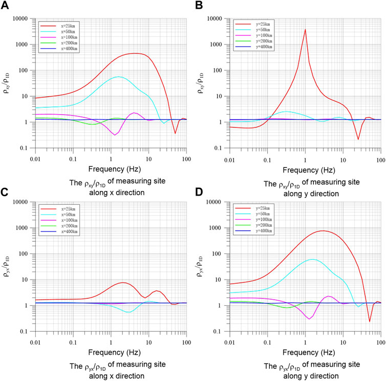
FIGURE 10. Ratio of the apparent resistivity of the 3D anomaly body together with inclined dipole source in the earth to the apparent resistivity of the 1D layered earth model for measuring sites of different offsets along x- and y-direction. (A) and (B) are the ρxy/ρ1D of measuring sites along x and y direction respectively; (C) and (D) are the ρyx/ρ1D of measuring sites along x and y direction respectively.
Figure 10C shows the ratio curve of
Figure 11 shows the spatial distribution of the ratio of the apparent resistivity calculated by superposition of the magnetotelluric response of the 3D low resistance anomaly and the x-direction inclined dipole source response in the layered earth model to the apparent resistivity of the 1D layered earth model, for frequencies of 10, 1 and 0.01 Hz, respectively. The range of the drawings is the same as that in Figure 9. The small white arrows in Figure 11 indicate the position of the electric dipole source in the earth, and the white step lines indicate the boundary of the 3D low resistance anomaly. It can be seen from the plot that the apparent resistivity change caused by the dipole radiation source at depth occurs in the area near the source, and the closer the source, the greater the anomaly. The apparent resistivity far away from the source is almost unchanged (the ratio is equal to 1). The anomaly in the intermediate frequency band has the maximum amplitude enhancement anomaly and a strong reduction anomaly (the ratio is far less than 1). The amplitude of the medium frequency band (f = 1 Hz) anomaly is the largest (0.01–30,000 times), and the expansion range is also large. The anomaly of
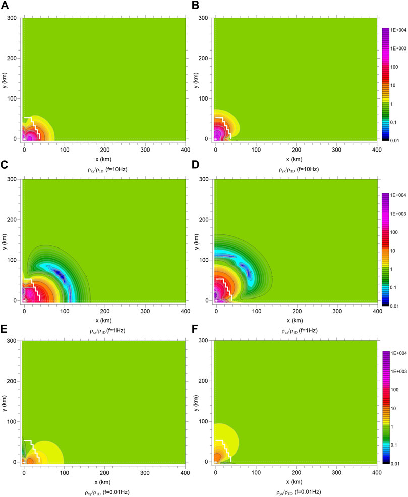
FIGURE 11. Contour plots of the ratio of apparent resistivity with 3D anomaly body together with inclined dipole source to the apparent resistivity of the 1D layered model. (A,C,E) are the ρxy/ρ1D at the frequency of 10 Hz, 1 Hz, 0.01 Hz respectively; (B,D,F) are the ρyx/ρ1D at the frequency of 10 Hz, 1 Hz, 0.01 Hz respectively.
It can be seen from the analysis of the above simulations that the observational data of magnetotelluric stations may contain seismogenic electromagnetic anomaly information. The characteristics of different types of seismic electromagnetic anomalies in magnetotelluric impedance response can be summarized as follows. In the seismogenic process, the change of formation resistivity (seismogenic resistivity anomaly) can produce a recognizable low-frequency (less than 1 Hz) apparent resistivity anomaly in magnetotelluric data. The anomaly is mainly a reduction of apparent resistivity from the normal value, and small amplitude enhancement anomalies may also be observed at various spatial sites. Although the amplitude of the anomaly is small, it may also be detected hundreds of kilometers (more than 200 km) away from the seismogenic center. However, if there is a low-frequency electromagnetic radiation anomaly at the same time, the influence of seismogenic low resistance anomaly may be completely masked in the low-frequency band due to the strong anomaly generated by dipole radiation in the seismogenic area. The anomaly produced by low-frequency electromagnetic radiation before earthquakes are characterized by a sharp increase of the apparent resistivity in the near-field zone, the phase approaching zero, and strong amplification of the anomaly by the presence of vertical source dipole components.
The influence of electromagnetic radiation before earthquakes included in magnetotelluric data on apparent resistivity depends on the proportion of each component of the radiation field in the spectral intensity of each component of the corresponding magnetotelluric field and will show different frequency and spatial characteristics from the response of a pure dipole source. For example, the response of a simple dipole source can be simply divided into a far-field zone and a near-filed zone according to frequency or offset, while the response of a dipole source radiation field contained in magnetotelluric data to apparent resistivity shows frequency selectivity, that is, anomalous amplitudes in the high-frequency and low-frequency bands are small, and the abnormal amplitude in the medium frequency band (0.1–50 Hz in this example) is largely due to the weak energy window of magnetotelluric field. In space, the response of the pure dipole source shows a small amplitude oscillation in the far-field area, which is difficult to identify in the magnetotelluric data. The manifestation of electromagnetic radiation in magnetotelluric response before earthquakes are mainly from the apparent resistivity enhancement anomaly with strong amplitude, and the anomaly amplitude decreases with the distance from the radiation source, but the apparent resistivity reduction anomaly with large amplitude may also appear for the data of different observation sites and different frequencies. The magnitude and spatial range of the influence of electromagnetic radiation on apparent resistivity before earthquakes are related to the intensity of the radiation sources. The stronger the radiation field intensity is, the larger the amplitude of apparent resistivity anomaly, and the wider the distribution range of anomaly. The calculation result of the source moment 1011A
The algorithm for 3D magnetotelluric modeling has adopted the strategy of magnetic field normalization for field component calculation, and the calculated strength for each field component may be different from the actual spectral intensity of each component measured at the station. However, the basic characteristics of electromagnetic radiation before earthquakes simulated by an electric dipole source in magnetotelluric response are valid.
In summary, electromagnetic impedance responses of a 3D low-resistance anomalous body which is used to simulate the resistivity change of strata in the seismogenic region, and an electric dipole which is used to simulate the seismogenic radiation source in horizontally layered earth model have been calculated, and the characteristics of electromagnetic impedance response with frequency and space over a large area have been analyzed quantitatively. The simulation results show that: 1) Visual resistivity anomalies of the 3D resistivity anomalous body appear in the frequency band below 5 Hz, with negative anomalies dominating in the frequency band below 1 Hz. The amplitude of the negative anomaly decreases with the increase of the offset distance, and the anomaly can be identified over 200 km. The measured data show that the resistivity often presents an abnormal decline feature before the earthquake, and the numerical simulation in this paper provides a theoretical basis for this phenomenon. 2) The vector electric dipole radiation source is equivalent to the electromagnetic radiation in the seismogenic region, and calculating and analyzing the electromagnetic impedance response. It is found that the component of tilted electromagnetic radiation in the y-direction will greatly enhance the detectability of electromagnetic anomalies. 3) Considering the electromagnetic radiation and the change of resistivity in the seismogenic area comprehensively, it is found that the medium frequency band (0.1–50 Hz) is the dominant frequency band for seismic electromagnetic anomalies. Around 1 Hz, the anomaly is more obvious and can be detected at a large spatial range.
The obtained results are of great significance for the observation of seismic electromagnetic anomalies, data processing, and analysis of the identification of electromagnetic anomalies in different seismogenic processes. In the future, we can analyze and compare data changes during earthquakes by combining measurement data from 30 ELF stations in the metropolitan area and the North-South seismic zone in China.
The original contributions presented in the study are included in the article, further inquiries can be directed to the corresponding author.
YF drafted the manuscript and the figures with the guidance of WH. All authors contributed to the completion of procedures, and discussion of this study, and provided feedback on the manuscript.
This work was supported by the National Natural Science Foundation of China (No. 41574064), Basic Research Funds from the Institute of Geology, China Earthquake Administration (No. IGCEA2002), and the Beijing Natural Science Foundation Project (No. 8212045).
The authors would like to express gratitude to EditSprings (https://www.editsprings.cn) for the expert linguistic services. We acknowledge the constructive reviews of the reviewers, and the useful summary and review by the editor JL. We also thank Professor PH (China Earthquake Network Center) for her guidance.
The authors declare that the research was conducted in the absence of any commercial or financial relationships that could be construed as a potential conflict of interest.
All claims expressed in this article are solely those of the authors and do not necessarily represent those of their affiliated organizations, or those of the publisher, the editors and the reviewers. Any product that may be evaluated in this article, or claim that may be made by its manufacturer, is not guaranteed or endorsed by the publisher.
Ding, J. H. (2009). Geomagnetic diurnal earthquake prediction method and earthquake cases. Beijing: Seismological Press.
Du, A. M., Zhou, Z. J., Xu, W. Y., and Yang, S. F. (2004). Generation mechanisms of ULF electromagnetic emissions before the ML=7.1 earthquake at Hetan of Xin Jiang. Chin. J. Geophys. 47, 832–837. http://www.geophy.cn/article/id/cjg_555.
Du, X. B. (2011). Two types of changes in apparent resistivity in earthquake prediction. Sci. China Earth Sci. 54 (1), 145–156. doi:10.1007/s11430-010-4031-y
Fan, Y., Tang, J., Zhao, G. Z., Wang, L. F., Wu, J. X., Li, X. S., et al. (2013). Schumann resonances variation observed from Electromagnetic monitoring stations. Chin. J. Geophys. 56, 2369–2377. doi:10.6038/cjg20130723
Gao, S. D., Tang, J., Du, X. B., Liu, X. F., Su, Y. G., Chen, Y. P., et al. (2010). The change characteristics of electromagnetic field before to after Wenchuan Ms8.0 earthquake. Chin. J. Geophys. 53, 512–525. doi:10.3969/j.issn.0001-5733.2010.03.005
Gao, S. D., Tang, J., and Sun, W. H. (2013). Electromagnetic anomaly before the Yingjiang MS5.8 and Myanmar MS7.2 earthquakes. Chin. J. Geophys. 56, 1538–1548. doi:10.6038/cjg20130512
Gao, Y., and Hu, H. (2010). Seismoelectromagnetic waves radiated by a double couple source in a saturated porous medium. Geophys J. Int. 181, 873–896. doi:10.1111/j.1365-246x.2010.04526.x
Gao, Y., Harris, M., Wen, J., Huang, Y., Twardzik, C., Chen, X., et al. (2016). Modeling of the coseismic electromagnetic fields observed during the 2004 Mw 6.0 Parkfield earthquake. Geophy. Res. Lett. 43, 620–627. doi:10.1002/2015GL067183
Hu, H., and Gao, Y. (2011). Electromagnetic field generated by a finite fault due to electrokinetic effect. J. Geophy. Res. 116, B08302. doi:10.1029/2010JB007958
Hu, K. Y., Hu, W. B., and Huang, Q. H. (2023). The electromagnetic wave fields induced by dipoles in the horizontally stratified medium. Chin. J. Geophys. 8, 1–12. Available at: https://doi.org/10.6038/cjg2023Q0775 (Accessed February 22, 2023). doi:10.6038/cjg2023Q0775
Huang, F. Q., Li, M., Ma, Y. C., Han, Y. Y., Tian, L., Yan, W., et al. (2017). Studies on earthquake precursors in China: A review for recent 50 years. Geodesy Geodyn. 8, 1–12. doi:10.1016/j.geog.2016.12.002.geog.2016.12.002
Huang, Q. H. (2002). One possible generation mechanism of co-seismic electric signals. Proc. Jpn. Acad. Ser. B 78, 173–178. doi:10.2183/pjab.78.173
Huang, Q. H., Ren, H. X., Zhang, D., and Chen, Y. J. (2015). Medium effect on the characteristics of the coupled seismic and electromagnetic signals. Proc. Jpn. Acad. Ser. B 91, 17–24. doi:10.2183/pjab.91.17.91.17
Li, M., Wang, Z. P., Lu, J., Tan, H. D., and Zhang, X. T. (2018). Estimating the equivalent dipole of the 2008 wenchuan Ms8.0 earthquake using observed electromagnetic ground signals. Earthquake 38, 49–60. http://dizhen.ief.ac.cn/CN/Y2018/V38/I1/49.
Ma, Q. (2002). The boundary element method for 3-D dc resistivity modeling in layered Earth. Geophysics 67, 610–617. doi:10.1190/1.1468622
Mao, T. N. (1986). Present status of electric-magnetic studies in earthquake science in China. Earthq. Res. China 30, 31–35. https://www.cnki.com.cn/Article/CJFDTOTAL-ZGZD198603005.htm.
Pan, H. W. (1998). Development and prospects of the earthquake electromagnetic observation system in China. Earthquake 18, 115–119. http://dizhen.ief.ac.cn/CN/Y1998/V18/IS1/115.
Qian, F. Y., Zhao, Y. L., Yu, M. M., Wang, Z. X., Liu, X. W., and Chang, S. M. (1982). Anomalous variation of apparent resistivity before earthquakes. Sci. China Earth Sci. 9, 831–839. http://www.cnki.com.cn/Article/CJFDTotal-ZBDZ198202004.htm.
Ren, H., Huang, Q., and Chen, X. (2016). Existence of evanescent electromagnetic waves resulting from seismoelectric conversion at a solid–porous interface. Geophys J. Int. 204, 147–166. doi:10.1093/gji/ggv400
Ren, H., Wen, J., Huang, Q., and Chen, X. (2015). Electrokinetic effect combined with surface-charge assumption: A possible generation mechanism of coseismic EM signals. Geophys J. Int. 200, 837–850. doi:10.1093/gji/ggu435
Wait, J. R. (1951). The magnetic dipole over the horizontally stratified Earth. Can. J. Phys. 29, 577–592. doi:10.1139/p51-060
Wang, J. J., Zhao, G. Z., Zhan, Y., Zhuo, X. J., Tang, J., Guan, H. P., et al. (2005). Observations and studies on EM phenomena caused by earthquake in China. J. Geodesy Geodyn. 25, 11–21.
Zhang, H. K., Shen, Q. X., Wu, W., Zhao, Y. L., and Mao, T. E. (1996). Research on dynamic prediction method of apparent resistivity in earthquake. Acta Seismol. Sin. 18, 340–345. https://www.dzxb.org/article/id/2e00a835-f6c7-47d4-8269-58f665298c71.
Zhang, X. M., Qian, J. D., Sheng, X. H., Liu, J., Wang, Y. L., Huang, J. P., et al. (2020). The seismic application progress in electromagnetic satellite and future development. Earthquake 40, 18–37. doi:10.12196/j.ISSN.1000-3274.2020.02.002
Zhao, G. Z., Wang, L. F., Tang, J., Chen, X. B., Zhan, Y., Xiao, Q. B., et al. (2010). New experiments of CSELF electromagnetic method for earthquake monitoring. Chin. J. Geophys. 53, 479–486. doi:10.3969/j.issn.0001-5733.2010.03.002
Zhao, G. Z., Wang, L. F., Zhan, Y., Tang, J., Xiao, Q. B., Chen, X. B., et al. (2012). A new electromagnetic technique for Earthquake monitoring CSELF and the first observational network. Seismol. Geol. 34, 576–585. doi:10.3969/j.issn.0253-4967.2012.04.004
Zhao, G. Z., Zhang, X. M., Cai, J. T., Zhan, Y., Ma, Q. Z., Tang, J., et al. (2022). A review of seismo-electromagnetic research in China. Sci. China Earth Sci. 65, 1229–1246. doi:10.1007/s11430-021-9930-5
Keywords: seismogenic resistivity anomaly, pre-earthquake electromagnetic emissions, electric dipole source response, magnetotelluric response, apparent resistivity
Citation: Fan Y, Hu W, Han B, Tang J, Wang X and Ye Q (2023) Characteristic identification of seismogenic electromagnetic anomalies based on station electromagnetic impedance. Front. Earth Sci. 11:1110056. doi: 10.3389/feart.2023.1110056
Received: 28 November 2022; Accepted: 25 April 2023;
Published: 15 May 2023.
Edited by:
Jie Liu, Sun Yat-sen University, Zhuhai Campus, ChinaReviewed by:
Yongxin Gao, Hefei University of Technology, ChinaCopyright © 2023 Fan, Hu, Han, Tang, Wang and Ye. This is an open-access article distributed under the terms of the Creative Commons Attribution License (CC BY). The use, distribution or reproduction in other forums is permitted, provided the original author(s) and the copyright owner(s) are credited and that the original publication in this journal is cited, in accordance with accepted academic practice. No use, distribution or reproduction is permitted which does not comply with these terms.
*Correspondence: Wenbao Hu, aHdiQHlhbmd0emV1LmVkdS5jbg==
Disclaimer: All claims expressed in this article are solely those of the authors and do not necessarily represent those of their affiliated organizations, or those of the publisher, the editors and the reviewers. Any product that may be evaluated in this article or claim that may be made by its manufacturer is not guaranteed or endorsed by the publisher.
Research integrity at Frontiers
Learn more about the work of our research integrity team to safeguard the quality of each article we publish.