
94% of researchers rate our articles as excellent or good
Learn more about the work of our research integrity team to safeguard the quality of each article we publish.
Find out more
ORIGINAL RESEARCH article
Front. Earth Sci., 22 June 2023
Sec. Cryospheric Sciences
Volume 11 - 2023 | https://doi.org/10.3389/feart.2023.1106621
This article is part of the Research TopicAdvances of Remote Sensing in Understanding Cryospheric Changes and ProcessesView all 6 articles
 Kehan Yang1,2,3,4*
 Karl Rittger2,5
 Keith N. Musselman2
 Edward H. Bair5
 Jeff Dozier6
 Steven A. Margulis7
 Thomas H. Painter8
 Noah P. Molotch1,2,9
Whereas many independent methods are used to estimate snow water equivalent (SWE) and its spatial distribution and seasonal variability, a need exists for a systematic characterization of inter-model differences at annual, seasonal, and regional scales necessary to quantify the associated uncertainty in these datasets. This study conducts a multi-scale validation and comparison, based on Airborne Snow Observatory data, of five state-of-the-art SWE datasets in the Sierra Nevada, California, including three SWE datasets from retrospective models: an INiTial REConstruction model (REC-INT), an improved REConstruction model based on the ParBal energy balance model (REC-ParBal), and a Sierra Nevada SWE REConstruction with Data Assimilation (REC-DA), and two operational SWE datasets from the U.S. National Weather Service, including the Snow Data Assimilation System (SNODAS) and the National Water Model (NWM-SWE). The results show that REC-DA and REC-ParBal provide the two most accurate estimates of SWE in the snowmelt season, both with small positive biases. REC-DA provides the most accurate spatial distribution of SWE (R2 = 0.87, MAE = 66 mm, PBIAS = 8.3%) at the pixel scale, while REC-ParBal has the least basin-wide PBIAS (R2 = 0.79, MAE = 73 mm, PBIAS = 4.1%) in the snowmelt season. Moreover, REC-DA underestimates peak SWE by −5.8%, while REC-ParBal overestimates it by 7.5%, when compared with the measured peak SWE at snow pillow stations across the Sierra Nevada. The two operational SWE products—SNODAS and NWM-SWE—are less accurate. Furthermore, the inter-model comparison reveals a certain amount of disagreement in snow water storage across time and space between SWE datasets. This study advances our understanding of regional SWE uncertainties and provides critical insights to support future applications of these SWE data products and therefore has broad implications for water resources management and hydrological process studies.
The spatial distribution of snow is important for water resources management, evaluation of regional climate models, biogeochemical cycling, and Earth’s energy balance. However, estimating the spatial distribution of snow water storage in mountainous regions, which is often measured as snow water equivalent (SWE), is challenging due to the heterogeneity of mountain terrain and high interannual variability in local climate (Dozier et al., 2016). While much effort has been made to develop feasible approaches for accurately estimating SWE over large mountain ranges, the performance of these methods has rarely been systematically evaluated using accurate validation datasets over time and space because of the difficulty in acquiring such datasets. Moreover, few studies have assessed the spatiotemporal characteristics of inter-model SWE differences at a fine spatial resolution (<1 km) at mountain-range scales.
Independent approaches to SWE reconstruction models have shown accurate SWE estimation when compared to snow courses and snow pillows. Reconstruction methods calculate SWE retrospectively from the time of satellite-observed snow disappearance back to peak SWE accumulation based on calculations of the potential snowmelt rate and depletion curve of the snow cover (Cline et al., 1998; Molotch et al., 2005; Molotch, 2009; Guan et al., 2013; Bair et al., 2016; 2018; Rittger et al., 2016). Early SWE reconstruction models were restricted to small catchments due to the limited availability of meteorological forcing data over mountainous terrain (i.e., solar and longwave radiation, air temperature, wind speed, and vapor pressure). The availability of large-scale, spatially-distributed forcing data (Xia et al., 2012a; 2012b) and the development of downscaling methods have facilitated the development of reconstruction models for larger mountain range, such as the Rio Grande headwaters (Molotch, 2009), California’s Sierra Nevada (Guan et al., 2013; Rittger et al., 2016; Bair et al., 2016), and the extratropical Andes Cordillera (Cornwell et al., 2016).
In terms of the accuracy of SWE estimates, SWE reconstruction models often outperform “forward” snow models because reconstruction models, unlike forward models, do not rely on precipitation forcing data, which are notoriously uncertain over mountainous areas (Raleigh and Lundquist, 2012; Slater et al., 2013). However, SWE reconstruction models do have unique limitations. For example, these models are only applicable in hindcast and only provide SWE information from peak accumulation through the snowmelt season. Hence, SWE reconstruction models are generally limited to applications in regions with distinct snow accumulation and ablation periods. Moreover, these models are sensitive to uncertainties in input meteorological forcing data and remotely sensed snow properties, such as fractional snow cover (FSCA) and snow albedo. For example, FSCA impacts the modeled energy flux calculation by allocating the snowmelt of each pixel and by determining the snow disappearance date (Raleigh and Lundquist, 2012). Interpolation of FSCA between measurements (e.g., infrequent overpasses or clouds) may propagate measurement errors into snowmelt calculation errors. Snow albedo strongly influences net solar radiation, the predominant energy source for snowmelt, which means uncertainty in snow albedo causes uncertainty in total energy available for snowmelt and therefore reconstructed SWE estimates (Bair et al., 2019).
The underlying SWE reconstruction approach has recently been merged with forward modeling approaches using batch-smoother data assimilation (DA) techniques (Durand et al., 2008a; Girotto et al., 2014a; Margulis et al., 2015). This approach accounts for the sources of uncertainties in snow observations (e.g., snow albedo, FSCA), and radiative and meteorological forcings like shortwave and longwave radiation, and precipitation. The DA approach estimates ensemble-based state variables (e.g., SWE and FSCA) over the entire snow accumulation and ablation seasons (Girotto et al., 2014a; Girotto et al., 2014b; Margulis et al., 2015). In the DA framework, a forward (reanalysis) land surface model is used to derive prior estimates of SWE (Xue et al., 2003). The prior SWE estimates are then updated using a particle batch-smother DA scheme based on a full season of satellite-derived FSCA observations (Margulis et al., 2015; 2016). The particle batch-smother approach, unlike the more common ensemble Kalman filter (Girotto et al., 2014a; Girotto et al., 2014b), is more appropriate for non-linear model systems and observations with higher order moments because it avoids the implicit assumptions that the state variables and measurements exhibit Gaussian distributions (Margulis et al., 2015).
In addition to the challenges to model distributed SWE at a fine scale over whole mountain ranges, it is also difficult to provide a comprehensive validation of the SWE datasets due to data availability limitations. While ground-based SWE observations from snow pillows and snow courses are widely used to validate these models (Guan et al., 2013; Margulis et al., 2015; Margulis et al., 2016; Schneider and Molotch, 2016), these point or transect scale observations do not capture the spatial variability of SWE over mountain watersheds (Molotch and Bales, 2005; 2006; Meromy et al., 2013). Given that in situ stations are typically sparsely distributed across the mountain range and mostly located in low and middle elevations (Yang et al., 2022), relying solely on in situ data for SWE evaluation does not provide a complete representation of SWE variance across the topographic variability of the mountain range (Molotch and Bales, 2006; Meromy et al., 2013). Furthermore, validation methods that rely on spatial interpolation of intensive snow surveys (Balk and Elder, 2000; Erxleben et al., 2002; Molotch et al., 2005; Molotch, 2009; Jepsen et al., 2012; Schneider and Molotch, 2016) are restricted to small areas and exclude steep slopes and dense forests because of the logistical challenges of intensive field surveys.
Recently, the Airborne Snow Observatory (ASO) has provided a new SWE dataset of unprecedented accuracy and spatial coverage that has likewise been seen as a good reference for basin scale SWE validation (Bair et al., 2016; Painter et al., 2016). Along with itres CASI 1500 visible-shortwave infrared imaging spectrometer, ASO uses a Riegl Q1560 airborne laser scanner to estimate snow depth by subtracting the snow-off from snow-on surface elevations at 3 m spatial resolution (https://airbornesnowobservatories.com/ as of 17 April 2023). The snow depth is then resampled to 50 m and multiplied by snow density as estimated by an in situ constrained physically based snow model—iSnobal (Marks et al., 1999) to generate spatially continuous SWE maps over watershed scales at 50-m spatial resolution. The snow depth has a low uncertainty of <2 cm at 50 m resolution when evaluated with 80 in situ observations over a relatively flat area near Tioga Pass, California (Painter et al., 2016). Given that most of the spatial variability in SWE is expressed in the snow depth (Lopez-Moreno et al., 2013), the final SWE product has achieved a high level of accuracy although the uncertainties of ASO SWE remain sensitive to errors in the modeled density estimation. While more thorough evaluation is needed, the ASO SWE is increasingly used as an independent ground “truth” validation dataset to evaluate other SWE data products at large basin scales (Bair et al., 2016; Oaida et al., 2019; Yang et al., 2022). It outperforms the traditional small-scale or point-scale SWE observations by providing spatially complete SWE estimates over large watersheds (Painter et al., 2016; Bormann et al., 2018). The longest ASO SWE record is available for the Tuolumne River Basin above the Hetch Hetchy Reservoir from 2013 to present. Each year, ASO acquires data from additional basins, and now covers most of the Sierra Nevada, as well as expanding into parts of the Rocky Mountains in Colorado and Wyoming, and even parts of Europe.
The objective of this study is to provide a comprehensive validation and inter-model comparison of five recently developed SWE products over an 11-year period in the Sierra Nevada of California. The following three criteria are used to select SWE products: 1) at least a decade of data availability across the entire Sierra Nevada; 2) spatial resolutions 1 km or finer, and 3) general applicability to other large mountain ranges globally. Two datasets rely on SWE reconstruction: Guan et al. (2013), which is a relatively early SWE reconstruction model, hereafter REC-INT (REConstruction-IniTial), and Bair et al. (2016) adapted from Rittger et al. (2016), hereafter REC-ParBal named after the primary energy balance model—ParBal. A third model, the Sierra Nevada SWE reanalysis, uses Data Assimilation (Margulis et al., 2016), hereafter REC-DA. To offer a baseline of SWE accuracy in the current water management system, this study includes two operational SWE datasets that rely on forward models: the Snow Data Assimilation System (SNODAS) (Carroll et al., 2001; Barrett, 2003) and the National Water Model (NWM) (version 1.2) (Gochis et al., 2018), hereafter NWM-SWE. These datasets rely on the most advanced modeling and remote sensing techniques at large mountain scale and represent some of the most accurate SWE estimates, with a spatial resolution of 1 km or finer.
To provide a comprehensive data evaluation, this study uses multi-scale validation datasets including spatially distributed ASO SWE data, transect-scale snow course SWE measurements, and point-scale snow pillow SWE observations. The latter two in situ datasets are distributed across the entire Sierra Nevada; only the ASO SWE data from the Tuolumne River Basin are used because the length of record there is the longest and observations are most frequent among the ASO acquisitions.
The Sierra Nevada is chosen as the study area given its abundant SWE datasets from in situ and remotely sensed observations, and from SWE estimation models. Snowmelt from the Sierra Nevada provides the main water supply for the State of California, which hosts one of the world’s largest economies and agricultural industries. This study focuses on areas of the Sierra Nevada above 1,500 m elevation because the snow below this elevation is ephemeral and less important from a water resources perspective (Bales et al., 2006; Guan et al., 2013; Rittger et al., 2016). The entire study area (Figure 1A) covers 19 Hydrologic Unit Code 8 (HUC8) snow-dominated watersheds with a total area of 42,021 km2. The average elevation of the study area is 2,270 m, ranging from 1,500 m to 4,410 m. The study area is summarized by five larger HUC6 sub-regions inclusive all HUC8 basins (Figure 1B and Table 1). The western slope of the Sierra Nevada is divided into three sub-regions based on the drainage areas of the Sacramento (northwest), the San Joaquin Rivers (center-west), and the Tulare Lake Basin (southwest). The eastern Sierra Nevada is divided into two sub-regions: northeast and southeast.
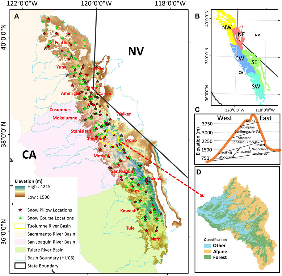
FIGURE 1. Overview of the study area. (A) The extent of the study domain represented by the elevation data. The locations of snow pillows (red stars), snow courses (green triangles), the Tuolumne River Basin above Hetch Hetchy (TRB, delineated by the yellow polygon); the blue lines extending to lower elevations indicate the boundary of each watershed (HUC8); and the yellow, blue, and green shaded regions represent the drainage areas of the Sacramento, San Joaquin, and Tulare Lake Basin, which further divide the western Sierra Nevada into three sub-regions: northwest (NW), centerwest (CW), and southwest (SW) (shown in sub-figure B). The eastern Sierra Nevada is divided into two sub-regions based on previous work (Huning and AghaKouchak, 2018): northeast (NE) and southeast (SE) sub-figures (B). (C) Typical cross-sections of ecoregions in the Sierra Nevada (modified from Sierra Nevada Ecoregional Plan 1999 (Meyer et al., 1999). (D) The classification of three land covers including “alpine”, “forest”, and “other”.
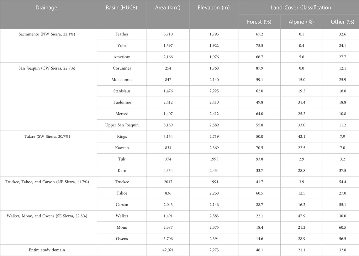
TABLE 1. Characteristics of the study domain above 1,500 m elevation.
The Sierra Nevada has a Mediterranean climate with dry summers and wet winters where 80% of the annual precipitation occurs in the cold months from October to May in the form of snow (Swain et al., 2016). Influenced by the prevailing westerly winds and orographic precipitation, the western windward side of the Sierra Nevada captures most of the moisture, while the eastern leeward side is much drier. The distribution of vegetation in the Sierra Nevada reflects the elevation and moisture gradients (Figure 1C). For the western slopes, the foothill zone is dominated by broad-leaved woodlands and evergreen shrublands. Coniferous forest covers most of the montane and subalpine zones. Pinyon-juniper woodlands and sagebrush communities are dominant on the east side of the Sierra Nevada below 2,000 m elevation (Meyer et al., 1999). In general, evergreen needle-leaf forest and shrub-lands are the two major land cover types in the Sierra Nevada, with most of the forest cover on the western slopes, where the annual precipitation is relatively high compared with the east side of the mountain range (Trujillo et al., 2012; Hansen et al., 2013).
The regions within the Tuolumne River Basin where the ASO campaign has conducted airborne snow surveys are highlighted in Figure 1A. This section of the Tuolumne River Basin above the Hetch Hetchy valley and reservoir (hereafter, TRB) in the central Sierra Nevada has an area of ∼1,200 km2 (Figure 1D). The average elevation of the TRB is 2,680 m, ranging from 1,500 m to 3,970 m. The average annual temperature and precipitation are about 4
To evaluate the accuracy of SWE datasets within different land cover types, the TRB is further classified into three main land cover types (Figure 1D): alpine, forest, and “other” based on the National Land Cover Data (NLCD) 2011 and the Shuttle Radar Topography Mission 1 Arc-Second Global Digital Elevation Model downloaded from https://earthexplorer.usgs.gov/as of 17 April 2023.
SWE reconstruction models are based on two premises: 1) satellite images of snow cover provide the spatial coverage and the date on which snow disappears from each grid cell, then 2) back-calculations of snowmelt yield estimates of SWE back to the date following the latest significant snowfall (Martinec & Rango, 1981). In regions where little snowfall occurs during the melt season, this date represents the maximum snow accumulation. Prescribing the date of maximum snow accumulation as day 0, then the SWE on day n can be calculated using Equation 3.1 and 3.2.
where Mj is melt on day j. SWE reconstruction methods differ in the way they identify the date when SWE goes to zero, the algorithm they use to measure and characterize the snow cover (either fractional or binary), and the methods and data sources they use to estimate daily melt. If, for example, FSCA is estimated, then the melt calculation incorporates it by multiplying the potential melt if the grid cell were entirely snow-covered by the FSCA, i.e.,
REC-INT (Guan et al., 2013) calculates SWE for each grid cell at 500-m resolution (Table 2). Potential melt
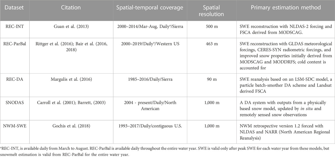
TABLE 2. Characteristics of the five SWE datasets compared in this study.
REC-ParBal (Bair et al., 2016; Bair et al., 2018; Rittger et al., 2016) covers the entire Western United States at the nominal MODIS spatial resolution of 463 m in the MODIS sinusoidal projection, and data are available in near-real time (Snow Today, 2022). This model explicitly accounts for changes in snowpack cold content and uses FSCA and grain size from MODSCAG, and an estimate of snow darkening from dust calculated with the MODIS Dust Radiative Forcing in Snow (MODDRFS, Painter et al., 2009). The meteorological forcings used in REC-ParBal are derived from the Global Land Data Assimilation System (GLDAS) at ¼
REC-DA is a 32-year (1985–2016) daily SWE reanalysis for the Sierra Nevada with a spatial resolution of about 100 m (Margulis et al., 2015; Margulis et al., 2016). REC-DA relies on a Land Surface Model (Simplified Simple Biosphere model, version 3; Xue et al., 2003) coupled with a Snow Depletion Curve model (Liston, 2004) (LSM-SDC) to derive the prior SWE and FSCA states, in which the radiative and meteorological forcings are taken from the downscaled NLDAS-2 (Xia et al., 2012a; Xia et al., 2012b). The particle batch smoother DA scheme is then used to update the prior SWE states directly based on the information extracted from FSCA observations retrieved from Landsat imagery (i.e., Landsat 5–8) (Cortez et al., 2014). This snow cover retrieval method doesn’t use canopy correction, and thus is a representation of only satellite viewable snow cover. In this respect, the DA scheme updates the precipitation weights used to disaggregate the distribution of precipitation based on the snow depletion data inherent in the FSCA time series. This is conceptually similar to, although numerically different from, the SWE reconstruction in areas with persistent snow cover that are given greater snow mass (Girotto et al., 2014a; 2014b), and thus we labeled this model by “REC” to distinguish with those models can be run in real-time.
The reanalysis approach differs from reconstruction methods in that it does not interpolate between FSCA measurements. Instead, it “fits” the observations in a Bayesian sense based on the postulated FSCA measurement error and associated likelihood of a given ensemble estimate. Because REC-DA uses a forward model of snow accumulation, the approach provides SWE estimates during the entire snow accumulation and ablation periods, making it more widely applicable than SWE reconstruction models (REC-INT and REC-ParBal that are only effective after peak snow accumulation). A new version of the SWE reanalysis dataset is recently available for download from the National Snow and Ice Data Center website (https://nsidc.org/data/wus_ucla_sr/versions/1) as of 17 April 2023. The dataset covers the entire Western United States from 1985 to 2021, with a spatial resolution of approximately 500 m (Fang et al., 2022).
SNODAS is a near real-time SWE modeling and data assimilation system developed and operated by the NOAA National Weather Service’s National Operational Hydrologic Remote Sensing Center (NOHRSC) (Carroll et al., 2001; Barrett, 2003). It provides daily SWE estimates at 0600 UTC for the contiguous United States at 1,000-m spatial resolution since water year 2004. Meteorological forcings for SNODAS are derived from a real-time Numerical Weather Prediction model (i.e., RUC2). The prior snow properties are derived from an energy-and-mass-balance and blowing snow model (Pomeroy et al., 1993) that are updated by available satellite- (e.g., GOES/AVHRR snow cover), airborne- (e.g., NOHRSC Airborne Gamma SWE) and ground-based (e.g., SNOTEL SWE, Cooperative Observer SWE and snow depth) snow observations in a data assimilation system (Carroll et al., 2001). The assimilation procedure is a simple nudging technique that calculates differences between estimated and observed SWE values and spatially interpolates the residuals to the model grid. Data are available at https://nsidc.org/data/g02158 as of April 17, 2023.
The National Water Model (NWM) is an extension of the Weather Research and Forecasting Hydrological model (WRF-Hydro) developed by the National Center for Atmospheric Research (Gochis et al., 2018). It relies on the Noah-MP Land Surface Model with observed precipitation and other meteorological inputs to simulate the land surface process (Niu et al., 2011; Yang et al., 2011). The SWE estimates of the NWM retrospective version 1.2 include a 25-year retrospective simulation from 1993 to 2017 at 1,000-m resolution, covering a large domain from latitude 19
Forty-six ASO flights occurred in the TRB from 2013 to 2017. This period covers various climate conditions including the 2013–2015 drought, the driest year on record (2015), the wettest year since 1983 (2017), and a moderate year (2016). Most of the ASO flights were operated from the near maximum snow accumulation to the snowmelt season, even into summer when all snow pillows reported zero SWE and snowpacks only remained in limited high-elevation regions. One ASO flight (8 July 2016) was removed in the model validation given the extremely low SWE reported (6 mm basin average SWE). Because the overlapping periods among SWE datasets and the ASO data are different, the entire validation period (2013–2017) has been divided into three sub-periods: 1) Period 1 from 2013 to 2014 with 17 ASO flights and all five SWE datasets; 2) Period 2 from 2013 to 2016 with 37 flights and four SWE datasets (REC-ParBal, REC-DA, SNODAS, and NWM-SWE); and, 3) Period 3 from 2013 to 2017 with all 45 flights but only three SWE datasets (REC-ParBal, SNODAS, and NWM-SWE).
To compare the SWE datasets with various resolutions and projections, all SWE datasets including ASO SWE data were first resampled to the same spatial resolution and coordinate system using bilinear interpolation. This study used a spatial resolution of 500 m (i.e., the median value among datasets used in this study) and the universal Transverse Mercator (UTM) zone 11N projection, which is the original coordinate system of ASO data in the Sierra Nevada.
To comprehensively evaluate SWE estimates, five statistical evaluation metrics were used: the coefficient of determination R-squared (R2), mean absolute error (MAE), root mean squared error (RMSE), root mean squared error normalized by basin average SWE derived from ASO SWE data (NRMSE), and the percentage bias (PBIAS). The first four metrics were used to represent the accuracy of SWE datasets at the grid scale, while the last metric was used to represent the overall accuracy of basin average SWE, with which water managers estimate the total snow water resource in a watershed. To reduce the impacts of geolocation errors caused by the resampling process, the SWE estimate with the smallest error relative to the ASO SWE inside a 3
There are 215 snow course sites located inside the study domain for the validation period of 2004 through 2014 (Figure 1A). Each snow course site includes 5–15 point-scale SWE measurements using a calibrated Federal Snow Sampler along an established transect (DeWalle and Rango, 2008). These data offer monthly SWE measurements near the first day of each month from January to May or June depending on the amount of snow remaining. Because both reconstructed SWE datasets (REC-INT and REC-ParBal) are only valid in the snowmelt season, only the snow course observations after peak SWE dates were used for validation. The peak SWE date was determined by the monthly time series of snow course measurements for each water year. Additionally, measurements with zero SWE were excluded. Given that some sites only have measurements taken in late winter or early spring (e.g., February, March, and April), there were 195 sites (i.e., 1861 station-years) that remained after removing measurements for the overlapping period of 2004–2014 as described above. These sites have an average elevation of 2,407 m, ranging from 1,478 m to 3,459 m.
The 107 snow pillow stations located inside the study domain have an average elevation of 2,464 m ranging from 1,570 m to 3,475 m. These data provide daily point-scale SWE observations for validation of the five SWE products. Similar to snow courses, all snow pillow observations before the peak SWE date were removed based on the daily time series SWE observations, and the zero SWE observations were also excluded. After removing these data, 50,628 station-years remained (i.e., 4,603 station-years for each water year) for data validation. It is worth mentioning that SNODAS incorporates snow pillow observations in the data assimilation system, and thus the comparison between the station-observed SWE and SNODAS modeled SWE is not strictly independent. However, we included SNODAS in the validation with snow pillow data to maintain consistency in the inter-model comparison. All snow pillow and snow course data were quality controlled and downloaded from the California Data Exchange Center (http://cdec.water.ca.gov) as of 17 April 2023.
To compare point-scale or transect-scale ground observations with gridded SWE datasets, this study used gap-filled gridded MODIS FSCA data (Rittger et al., 2020) (resampled to 500 m from its native 463 m resolution using bilinear interpolation) to scale the ground observations to the grid scale, which can improve the representativeness of SWE measurements at the grid scale (Schneider and Molotch, 2016). The same five statistical metrics (i.e., R2, MAE, RMSE, NRMSE, and PBIAS) were calculated to quantitatively evaluate gridded SWE values from SWE data products using FSCA scaled ground SWE observations. PBIAS for this analysis does not strictly represent the basin as these point or transect-scale observations represent only a very small portion of the basin. All the calculations were conducted using SWE grids at the 500 m resolution within a 3 × 3 grid-cell analysis window (see Section 3.2.1).
To compare the three validation results using the same criteria, we applied the station-year method for the ASO validation in Period 1 when all five datasets were available, in which each grid-by-grid comparison was seen as one station-year (i.e., one grid is seen as one site). The statistical results are reported in Supplementary Table S1. The ASO validation was equivalent to 62,728 station-years of data. Then, we used the average value of each statistical evaluation metric for the ASO, snow course, and snow pillow validations to represent the overall accuracy of the five SWE data products. Because the coverage, the scale, and the accuracy of the validation datasets were different, it is likely that the average estimate of the three validation results is not representative. Therefore, we also included the Taylor-diagram of each validation to provide a more intuitive comparison between different SWE datasets. The Taylor-diagram is a graphical evaluation diagram that provides a statistical summary of how well the predicted value (i.e., modeled SWE) matches observations (i.e., validation datasets) in terms of the Pearson’s correlation coefficient (r), RMSE, and standard deviation (Taylor, 2001).
To compare SWE datasets in terms of the spatial and temporal variability of SWE in the Sierra Nevada, the following five estimates across the study domain were calculated and compared: 1) Daily time series of Sierra-wide average SWE and snow water storage (SWS) (i.e., the volume of snowpack water as derived from the product of basin average SWE and total basin area); 2) 1 April SWE and SWS. These were compared because of their importance in water management and water supply forecasting in California; 3) elevational distribution of SWS on the first day of each month from April through August; 4) 11-year average SWE for the entire study domain and the five sub-regions (NW, CW, SW, NE, and SE Sierra with detailed information referring to Figure 1A and Table 1), and, 5) 11-year average spatial distribution of pixel-wise peak SWE, which is the maximum SWE estimate on a grid cell basis over the entire water year using all available daily SWE estimates. The pixel-wise peak SWE can represent the maximum snow water resources received by the entire mountain range throughout each water year (Margulis et al., 2016).
In Period 1, when all the five datasets were available, REC-DA (i.e., the SWE reanalysis with data assimilation) showed the best performance of the five SWE products through grid-by-grid comparison with ASO SWE in the TRB, closely followed by REC-ParBal, which had an overall smaller basin-wide PBIAS than REC-DA (Table 3). Both REC-DA and REC-ParBal explained a very significant amount of the spatial variance of the ASO SWE data, with mean R2 values of 0.93 and 0.85, respectively. The other reconstruction SWE product, REC-INT, was the third most accurate dataset in nearly all statistical comparisons (Table 3), explaining 70% of the spatial variance of the ASO SWE data but with a large −34% overall PBIAS.
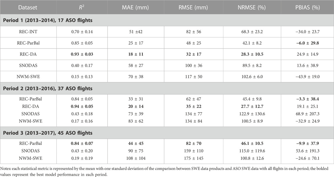
TABLE 3. Summary of the daily validation using ASO SWE data in the TRB for Period 1 (2013–2014) with 17 flights, Period 2 (2013–2016) with 37 flights, and Period 3 (2013–2017) with 45 flights.
Both operational models (SNODAS and NWM-SWE) showed significantly lower accuracy in the comparison for most statistical comparisons. SNODAS and NWM-SWE only explained 40% and 15% of the variance of ASO SWE on average, with an overall PBIAS of 13.6% and −43.9%, respectively. Although SNODAS had a smaller PBIAS than REC-INT and REC-DA, it had the largest standard deviation, meaning the overall basin-wide bias for SNODAS had a high variance and its performance was much less robust. Of all five SWE datasets, NWM-SWE had the lowest accuracy.
Periods 2 and 3 results were similar to the results shown for Period 1. In Period 2, when four SWE datasets (REC-ParBal, REC-DA, SNODAS, and NWM-SWE) were available, the average values of R2 and NRMSE for these four datasets were similar compared with those in Period 1, and the values of MAE and RMSE were slightly higher, which was reasonable given that Period 2 included Water Year (WY) 2016 with higher snow accumulation than 2014 and 2015. Consistently, the three datasets (i.e., REC-ParBal, SNODAS, and NWM-SWE) that were available in Period 3 also exhibited similar accuracy compared with their performance in Periods 1 and 2.
Figure 2 shows seasonal and interannual variability in the accuracy of the SWE datasets. The accuracy of REC-DA and REC-ParBal were relatively consistent interannually, regardless of climatic conditions (i.e., wet versus dry years). REC-DA showed the most robust performance, with nearly uniform R2 through the season (Figure 2A). REC-DA exhibited decreases in MAE towards the end of the snowmelt season (Figure 2E), and small positive basin-wide PBIAS values in all years except for the extremely dry year of 2015 when REC-DA, REC-ParBal, and SNODAS all exhibited highly variable PBIAS. REC-ParBal’s R2 values paralleled those of REC-DA, with slightly worse performance toward the beginning and the end of the snow season. Similarly, REC-INT had an increasing trend of R2 from the beginning to the middle of the snowmelt season, followed by a decreasing trend, indicating REC-INT better captured SWE spatial variance during the middle of the snowmelt season.
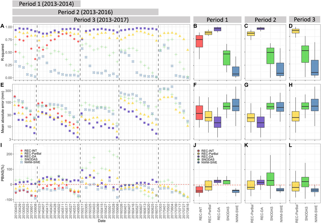
FIGURE 2. The variability of SWE data accuracy verified against ASO SWE data in the TRB for all three periods. (A, E, I) represent R2, mean absolute error, and PBIAS, respectively, while the boxplots in the right panel (B–H, J–L) summarize the overall validation results for each period.
The two operational datasets showed similar performance in capturing SWE variance among different water years combined with a decreasing trend in R2 towards the end of each melt season, indicating the performance of both models degraded for low snow periods. The performance of SNODAS exhibited high interannual variability: SNODAS underestimated basin average SWE for all 10 ASO flights in WY 2016, a wet year, but overestimated SWE for all ten flights in WY 2015, a dry year. SNODAS had a slightly better performance than NWM-SWE for most flights except for WY 2015, when SNODAS showed very high positive PBIAS and higher MAE than NWM-SWE. NWM-SWE had a relatively high R2 early in the snow season but its R2 dropped very quickly as the season progressed. NWM-SWE exhibited a consistently negative bias throughout the comparison period, as it underestimated basin average SWE for 41 out of 45 ASO flights.
Figure 3 shows the spatial distribution of average differences between each data product and ASO SWE data for the TRB in Period 1. The statistical evaluation results are summarized for alpine, forest, and other land cover types in Table 4. Compared to the other models, REC-DA had the lowest SWE errors indicated by the low MAE and RMSE in Table 4 for all three land cover types, and the lighter red (negative) and blue (positive) SWE errors in Figure 3, though it had an obvious overestimation for some alpine and forest regions. REC-DA had an overall PBIAS of 20.3%, 36.8%, and 2.7% for alpine, forest, and other (i.e., not forest or alpine) land cover classifications. Within these three land cover classes, REC-DA explained 0.88, 0.80, and 0.90 of the ASO SWE spatial variance, respectively.
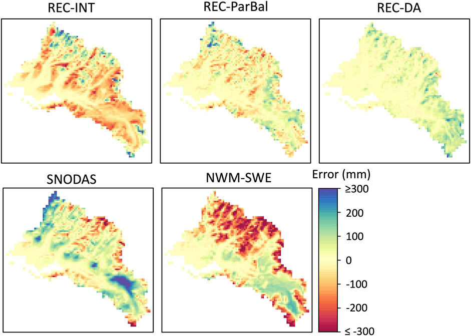
FIGURE 3. Spatial distribution of average SWE residuals derived from the five SWE datasets in Period 1 with 17 ASO SWE flights.
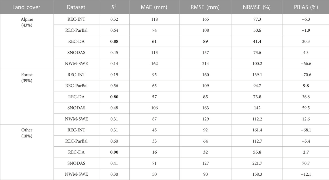
TABLE 4. Summary of SWE validation across alpine, forest, and “other” land cover types using ASO SWE data in Period 1. For the 17 ASO flights in Period 1, the validation pairs between each SWE data product and ASO data at 500 m resolution are equivalent to 62,728 station-years. The bold values represent the best performance of the five datasets.
Both REC-ParBal and REC-INT exhibited positive and/or negative errors that were notably higher than REC-DA, though the magnitude of the SWE residuals for REC-ParBal was smaller than REC-INT overall (Figure 3 and Table 4). Within the three different land cover types, REC-ParBal exhibited relatively consistent accuracies as revealed by the relative evaluation metrics R2, NRMSE, and overall basin-wide PBIAS, while the performance of REC-INT varied considerably. REC-INT and REC-ParBal showed the best performance in alpine regions. REC-ParBal showed similar accuracy in forested and “other” land cover classes, though the magnitude of residuals was higher in forested regions. REC-ParBal had the smallest PBIAS relative to other models in alpine and forested regions with values of −1.9% and 9.8%, respectively. REC-ParBal, however, exhibited a slightly higher PBIAS (−5.4%) compared to REC-DA (i.e., PBIAS = 2.7%) in the “other” land cover type.
The two operational datasets (i.e., SNODAS and NWM-SWE) exhibited relatively large SWE errors in forested and alpine regions (Figure 3). While SNODAS had a positive PBIAS for all three land cover classes (4.3% for alpine, 59.5% for forest, and 70.7% for other), it still underestimated SWE in many places (red pixels in Figure 3). Overall, SNODAS showed its best performance in alpine regions and had similar accuracy over forested and “other” land cover classes. NWM-SWE exhibited significant SWE underestimation in alpine (PBIAS = −66.6%) and “other” (PBIAS = −12.1%) regions, but it overestimated SWE in forested regions (PBIAS = 12.6%). Generally, NWM-SWE exhibited comparable accuracy over forested and “other” land cover classes and was the least accurate in alpine regions.
Validation of the five SWE datasets with ground measurements (i.e., snow course and snow pillow) covers the entire study domain of the Sierra Nevada shown in Figure 1A for an 11-year period (2004–2014). Like the validation results in the TRB with ASO SWE data, REC-DA and REC-ParBal performed better than the other models compared to snow course data (Figure 4) and snow pillow data (Figure 5). On average, REC-DA explained 89% and 87% of the variance in snow course and snow pillow SWE measurements with a 1.3% and −0.4% PBIAS, respectively while REC-ParBal explained 85% and 87% of the variance in snow course and snow pillow SWE measurements with 8.5% and 5.5% PBIAS. The MAE and RMSE for REC-DA were slightly higher in the validation with snow pillows than snow courses, but the NRMSE (30.0%) was the same.
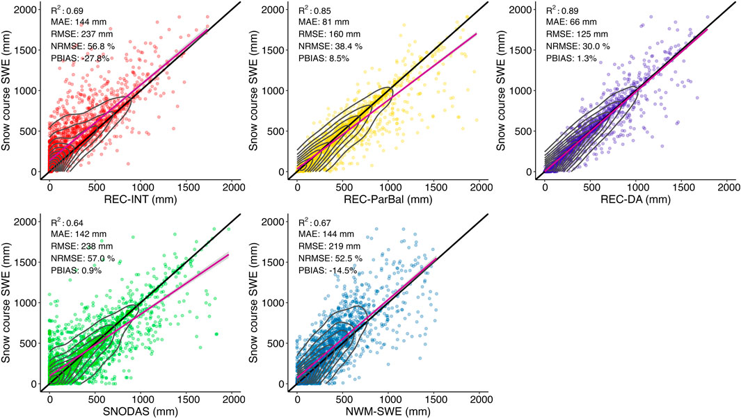
FIGURE 4. The comparison of gridded SWE extracted from SWE datasets against snow course SWE (scaled by fractional snow-covered area). A total number of 1861 station-years were compared. The black line represents the locations where FSCA-scaled snow course SWE equals to SWE datasets (1:1 line); the red line represents the best linear-fit; the gray contour represents the density of points in the scatter plots (i.e., the number of points per unit area).
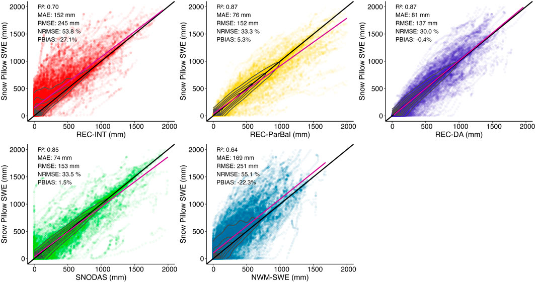
FIGURE 5. The comparison of gridded SWE extracted from SWE datasets against snow pillow SWE (scaled by fractional snow-covered area). A total of 50,628 station-years was compared. The black line represents the locations where FSCA-scaled snow pillow SWE observations are equal to SWE datasets (1:1 line); the red line represents the best linear fit; the gray contour represents the density of points in the scatter plots (i.e., the number of points per unit area). Because SNODAS assimilated snow pillow observations in the SWE estimation model, it had a much better performance when validated with snow pillow SWE observations compared with using other independent validation datasets (i.e., ASO SWE data and snow course SWE measurements). The validation for SNODAS here is not strictly independent.
REC-INT performed very consistently when compared to snow course data and snow pillow data, explaining 69% and 70% of the variance respectively. RMSE for REC-INT was 237 mm and 245 mm respectively at the snow course and snow pillow sites. REC-INT had a 27.8% PBIAS and NRMSE of 56.8% at snow course sites, and −27.1% PBIAS and NRMSE of 53.8% at snow pillow sites.
The two operational SWE datasets, SNODAS and NWM-SWE, had comparable performance to REC-INT, explaining 64% and 67% of the variance of snow course SWE, with 0.9% and −14.5% PBIAS, respectively. The MAE and NRMSE were 142 mm and 57.0% for SNODAS, and 144 mm and 52.5% for NWM-SWE, respectively. The dispersed distribution of SNODAS SWE in Figure 4 indicates considerable variation in SWE errors, particularly for the lower SWE observations, while NWM illustrated a consistent small underestimation, which was also true in the comparison with snow pillow data (Figure 5). On average, NWM-SWE performed slightly poorer at snow pillow locations than at snow courses. Because SNODAS ingested snow pillow observations in the data assimilation, its comparison with snow pillow SWE measurements does not provide an independent assessment. It is noticed that SNODAS was still less accurate than REC-DA at snow pillow sites (Figure 5).
To summarize the multi-scale validation results presented above, we synthesized the validations with ASO SWE (refer to Supplementary Table S1 for the station-year metrics), snow course, and snow pillow and used the average value of each statistical evaluation metric to represent the overall accuracy of the five SWE data products (Table 5) and their performance over different land cover types (Table 6). The individual validation was summarized by Taylor-diagrams in Figure 6.
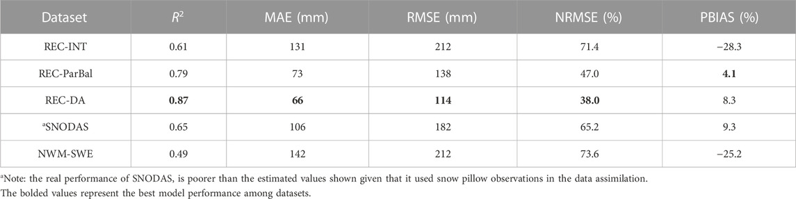
TABLE 5. Summary of the validation results of five SWE data products using multi-scale validation datasets including ASO SWE, snow course SWE, and snow pillow SWE. Each statistical metric is represented by the average value of the three validations, including 62,728 station-years of ASO flights in period one, 1861 station-years of snow course data, and 50,628 station-years of snow pillow data.
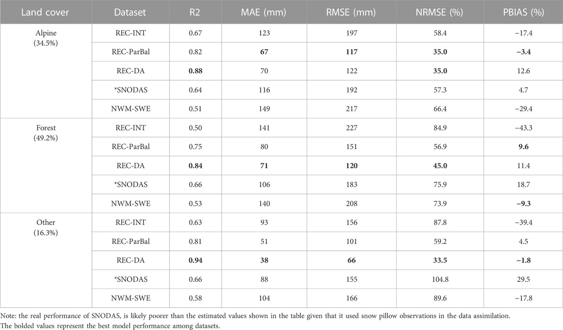
TABLE 6. Summary of SWE dataset validation across the three land cover classifications including alpine, forest, and “other” (i.e., not forest nor alpine). Each statistical metric is represented by the average value of the three validations, including 62,728 station-years of ASO flights in period one (Table 4), 1861 station-years of snow course data, and 50,628 station-years of snow pillow data. The number and proportion of validation pairs for each land cover classification are labeled in the table.
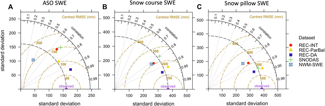
FIGURE 6. Taylor diagrams of the five SWE datasets in the validations with ASO SWE, (A) snow course SWE (B) and snow pillow SWE (C). Three statistical metrics including the R, RMSE, and standard deviation were used to quantify the agreement between the modeled (i.e., five SWE datasets) and observed (i.e., validation datasets) SWE estimates. The SWE datasets are represented by different shapes and colors, while the validation SWE data is displayed by the purple circle labeled “observed”. The real performance of SNODAS is likely poorer than the estimated values shown in the table given that it used snow pillow observations in the data assimilation.
REC-DA consistently had the highest correlation and lowest RMSE compared with three validation datasets, followed by REC-ParBal (Figure 6). The variability of ASO SWE data was much lower than that of snow course SWE and snow pillow SWE, as indicated by the lower standard deviation of observed ASO data in Figure 6. Among the five datasets, only NWM-SWE underestimated the variability of ASO SWE. SWE products showed consistent accuracy when validated with snow course SWE and snow pillow SWE, with the exception of SNODAS (green cross in Figures 6B, C), which ingested snow pillow observations into its data assimilation. REC-ParBal and SNODAS showed higher variability than snow pillow and snow course SWE on average, as indicated by the higher standard deviation than observed in Figures 6B, C, while the SWE values of the other three datasets showed lower variability.
REC-DA, the model run at the highest spatial resolution, showed the highest accuracy among the five SWE products in the pixel-by-pixel comparison, but it had an overall positive basin-wide PBIAS (8.3%). It explained 87% of the variance in observed SWE from the validation datasets, ranging from 89% in snow course SWE to 86% in ASO SWE, with 66 mm MAE, and 38.0% NRMSE (Table 5). Among three land cover types, REC-DA performed best within the “other” land cover types and the worst in forested regions (Table 6).
REC-ParBal exhibited the second-best performance with the lowest PBIAS overall. It explained 79% of the variance in the validation datasets, ranging from 64% in ASO SWE to 87% in the snow pillow SWE, with 73 mm MAE, 47.0% NRMSE, and a small 4.1% PBIAS (Table 5). Among three land cover types, REC-ParBal indicated the best performance in alpine regions (Table 6), with 35.0% NRMSE (31% lower than average), and showed comparable performance within forested and “other” land cover types. Additionally, REC-ParBal showed better performance than REC-DA in alpine regions.
REC-INT was the third-best dataset that explained 61% of the variance in the validation datasets, ranging from 45% in ASO SWE to 70% in snow pillow SWE, with 131 mm MAE, 71.4% NRMSE, and a −28.3% PBIAS overall (Table 5). Similar to REC-ParBal, REC-INT also had the best performance over alpine regions among three land cover types, with 58.4% NRMSE (13% lower than average). REC-INT showed the worst performance in forested regions, with a relatively large negative PBIAS (i.e., −43.3%) overall.
SNODAS was less accurate than the above three models and was the fourth-best in this study. It explained 65% of the variance in observed SWE from the validation datasets, ranging from 47% in ASO SWE to 85% in snow pillow SWE. However, the high variance explained in snow pillow SWE by SNODAS was very likely overestimated, as SNODAS used snow pillow data in its data assimilation. It had 106 mm MAE, 65.2% NRMSE, and 9.3% PBIAS overall. SNODAS also had a better performance than NWM-SWE over alpine regions, with 57.3% NRMSE (7.9% lower than average) (Table 5). SNODAS showed the worst performance in the “other” land cover type, with a large positive 29.5% PBIAS overall.
NWM-SWE showed the least accuracy that explained only 49% of the variance in all three validation datasets, ranging from 15% in ASO SWE to 67% in snow course SWE, with 142 mm MAE, 73.6% NRMSE, and −25.2% PBIAS overall (Table 5). Although it showed a quite similar accuracy to REC-INT and SNODAS at snow pillow and snow course sites, its comparison with ASO data illustrated that NWM-SWE failed to capture the spatial variance in ASO SWE. NWM-SWE exhibited the lowest accuracy in alpine regions, with a large negative bias (−29.4%), and it showed comparable accuracy within forested and “other” land cover types.
Sierra-wide average SWE exhibited significant interannual variability over the 11-year record (2004–2014) with the greatest snow accumulation in WY2011 and the lowest in WY 2014 (Figure 7). Overall, the daily Sierra-wide average SWE for all five datasets showed good agreement, particularly in the period after 1 May toward the end of snow season. We only included SWE estimates from 1 April to the end of snowmelt season for REC-INT and REC-ParBal given that the SWE estimates of these two datasets were not valid for the snow accumulation period. 1 April was used as a reasonable early bound on the peak SWE date to include the two reconstruction SWE products in the comparison, although the peak SWE dates vary spatially.
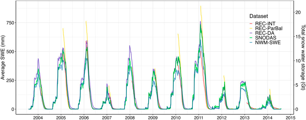
FIGURE 7. Time series of Sierra-wide average SWE and total snow water storage (SWS) for the 11-year overlapping period of 2004–2014. SWS is the product of the average SWE and the total area of the study domain, representing the snow water availability in the mountain range. Because REC-INT and REC-ParBal are only valid from peak SWE timing onward, we used 1 April as a reasonable early bound on the peak SWE date to exclude their SWE estimates before 1 April.
The average SWE values for REC-DA, SNODAS, and NWM-SWE were similar in the early winter, and the differences between the SWE products began to increase approaching the timing of maximum SWE. REC-DA and SNODAS had comparable annual peak SWE values, both of which were much higher than NWM-SWE. Once SWE began to decrease, the basin-wide average SWE for REC-INT and REC-ParBal tended to drop earlier than the other three datasets. This was particularly notable in WY2011 whereby it can be observed that the other three datasets were still accumulating snow whereas REC-INT and REC-ParBal exhibited a rapid SWE decline.
Of the five datasets, NWM-SWE and REC-INT typically had the lowest average SWE. REC-ParBal showed the greatest Sierra-wide average SWE in April to early May, and the values were significantly higher than the other SWE products. This result is somewhat counter-intuitive in that the aforementioned product validation results indicated that REC-DA had a larger PBIAS than REC-ParBal. One reason for this discrepancy is that we only validated SWE products after peak SWE so the majority of the validation data were acquired from May to the end of the snow season when REC-DA actually had the greatest SWE (Figure 7). We compared the maximum SWE values at snow pillow stations with the peak SWE estimates from REC-DA and REC-ParBal (Supplementary Figure S1). The results showed that REC-DA underestimated peak SWE by −5.8%, while REC-ParBal overestimated it by 7.5% (Supplementary Figure S1), suggesting that the true Sierra-wide maximum SWE values probably lie somewhere between the SWE estimates from REC-ParBal and REC-DA.
REC-ParBal had the highest 1 April SWE for 8 out of 11 years among all five datasets (Figure 8). On average, the 1 April SWE for REC-ParBal was 43% higher than NWM-SWE, which had the lowest value in 7 out of 11 years. Moreover, 1 April SWE for REC-INT, REC-DA, and SNODAS was 27%, 22%, and 29% lower than that of REC-ParBal, respectively. Section 4.4.3 describes in detail the regional SWE that led to these differences. The 11-year 1 April SWE for the five SWE data products exhibited high interannual variability. For the driest year (WY 2014), the average SWE value was 107 mm, ranging from 64 mm to 173 mm derived from REC-INT and REC-ParBal, respectively. For the wettest year (WY 2011), the average SWE value was 685 mm, ranging from 505 mm to 896 mm derived from REC-INT and REC-ParBal, respectively.
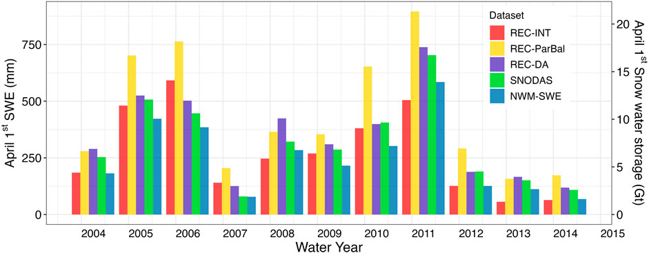
FIGURE 8. 1 April SWE and snow water storage (SWS) for the study domain derived from the five SWE datasets for an 11-year overlapping period.
The distribution of snow water storage (SWS) across the Sierra Nevada varies at different elevations among various SWE data products between 1 April and 1 August (Figure 9). On 1 April, REC-DA, SNODAS, and NWM-SWE estimated maximum SWS in the elevation band of 2,500–2,600 m, while REC-INT and REC-ParBal estimated maximum SWS at lower elevations around 2,000–2,100 m. REC-DA estimated similar SWS to SNODAS for elevations below 2,900 m, but slightly greater SWS at elevations around 2,900–3,800 m. NWM-SWE estimated much lower SWS than REC-DA and SNODAS throughout all elevation bands. REC-INT and REC-ParBal exhibited significantly different distributions compared with the above three datasets. REC-ParBal estimated notably high SWS at elevations between 1,600 and 2,600 m which are primarily forested regions in the western Sierra Nevada (Figure 1C), but less so in the eastern Sierra Nevada. These elevations are where most of the area of the Sierra Nevada lies (Figure 9). REC-INT also estimated higher SWS than the other three datasets (REC-DA, SNODAS, and NWM-SWE) in these elevations. Additionally, REC-INT exhibited much lower SWS for elevations between 2,200 and 3,000 m than the other four datasets.
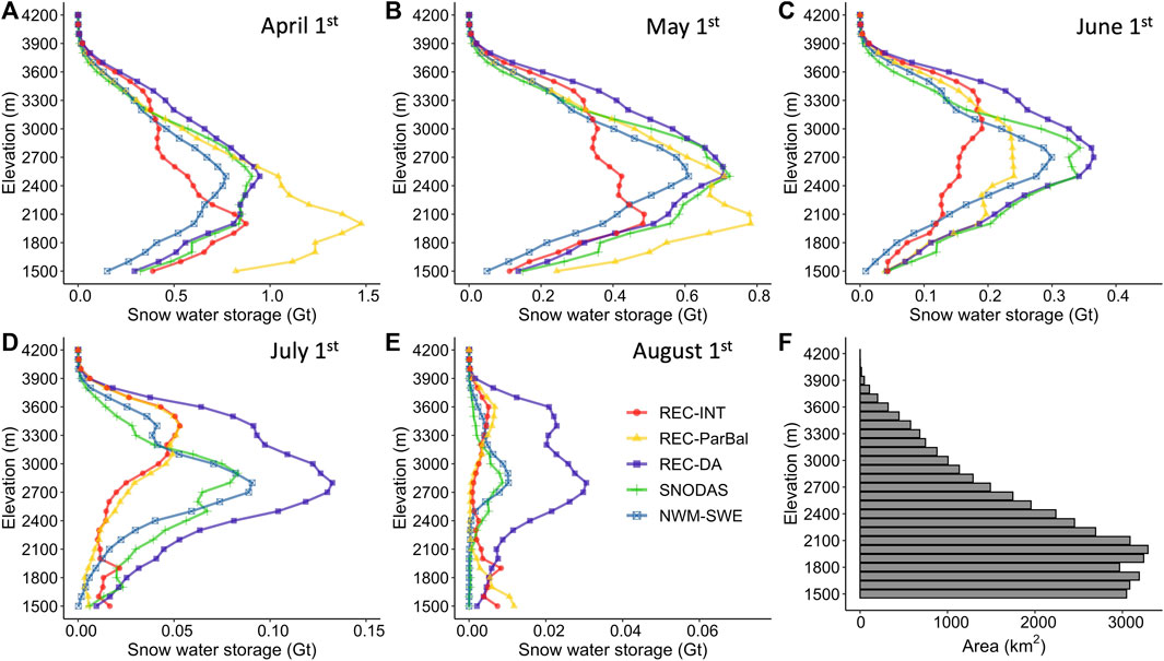
FIGURE 9. The monthly elevational distribution of the 11-year average seasonal variability of total snow water storage (SWS) on the first day of April through August. The interval of each elevation band is 100 m, ranging from 1,500 m to 4,300 m. The integration of each line represents the total SWS for the study domain.
This elevational pattern of SWS changed from 1 April to 1 May, with the greatest SWS decreases observed at middle to low elevations around 2,000 m–2,500 m. REC-DA, SNODAS, and NWM-SWE still exhibited similar distributions, and NWM-SWE estimated a relatively lower SWS, particularly at elevations below 3,000 m. Consistent with the pattern on 1 April, REC-ParBal estimated high SWS at elevations below 2,300 m where the largest areas in the Sierra Nevada occurs (Figure 9), while REC-INT estimated the lowest SWS around 2,200–3,000 m among all datasets.
On 1 June, REC-DA, SNODAS, and NWM-SWE exhibited similar distributions, with SWS for REC-DA primarily centered at 2,700–3,000 m. Consistently, REC-DA had the highest SWS, followed by SNODAS, while NWM-SWE estimated the lowest SWS of the three datasets. The SWS for REC-ParBal at elevations below 3,000 m corresponding to all elevations in the NW (i.e., Sacramento basins) decreased from 1 May to 1 June, indicating a much faster snowmelt rate estimated by REC-ParBal for this elevation range than other datasets. The maximum SWS for REC-INT shifted dramatically from low elevations (2,000–2,100 m) to high elevations (3,000–3,100 m) during this month.
Towards the end of snowmelt season (1 July and 1 August), the centroid of SWS for all five datasets moved to higher elevations, although their elevational distributions were still diverse. REC-DA estimated much higher SWS than the other four datasets and had the highest SWS at middle elevations around 2,700 m. Although the distribution of SWS for SNODAS and NWM-SWE was similar to that for REC-DA, their SWS estimates were much smaller. For these 2 months, REC-INT and REC-ParBal centered at higher elevations around 3,400–3,500 m with very similar SWS distributions.
The daily 11-year average SWE from 1 April through 31 August varies for the entire study domain and five sub-regions: southeast (SE), northeast (NE), southwest (SW), central-west (CW), and northwest (NW) Sierra (Figure 10). REC-DA had the greatest SWS across the Sierra between May 1 through the end of August. It had the highest SWS estimates for the sub-regions of CW (most dates), SW, and particularly the SE Sierra where the overall elevation is high, and the forest cover is low (Table 1, Figure 1C). REC-INT had the lowest SWS in the CW and SW where the average elevation is high, and it had a relatively high SWS from 1 April to 1 May in the NW. REC-ParBal generally estimated greater SWS than REC-INT, with significantly greater SWS in April for the northern Sierra (NE and NW). During the month of April, which is particularly important from a water resource management perspective, REC-ParBal SWS estimates were notably greater than the other four SWE products.
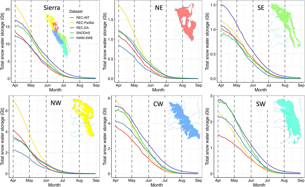
FIGURE 10. Time series of the 11-year average total snow water storage (SWS) for the entire study domain and five sub-regions. NE, SE, NW, CW, and SW represent the northeast, southeast, northwest, central-west, and southeast Sierra, respectively. The dashed gray lines represent the first day of each month from April through August. 1 Gt (gigaton) is equivalent to 109 m3 of water.
SNODAS had similar SWS to REC-DA in the northern Sierra (NE and NW) throughout the snowmelt season, but significantly lower SWS than REC-DA in the SE and CW. NWM-SWE had the lowest SWS in the northern Sierra (NE and NW) but exhibited moderate SWS values for the central and southern Sierra (CW, SW, and SE). In terms of the time series of total SWS across the entire Sierra (Figure 10), NWM-SWE exhibited the lowest SWS from 1 April to 1 May, while REC-INT was the lowest from mid-May towards the end of the snowmelt season.
The spatial distributions of the 11-year average pixel-wise peak SWE (hereafter maximum SWE) (Figure 11) were consistent with the findings described above (Figure 9 and Figure 10). REC-DA, SNODAS, and NWM-SWE showed a very similar spatial distribution of maximum SWE and the patterns of the interannual variability in maximum SWS while the magnitude of maximum SWE for these three datasets was different (Figures 11). REC-DA usually had the highest estimates (18.2 ± 8.5 Gt) while NWM-SWE usually was the lowest (13.6 ± 6.9 Gt) among these three datasets.
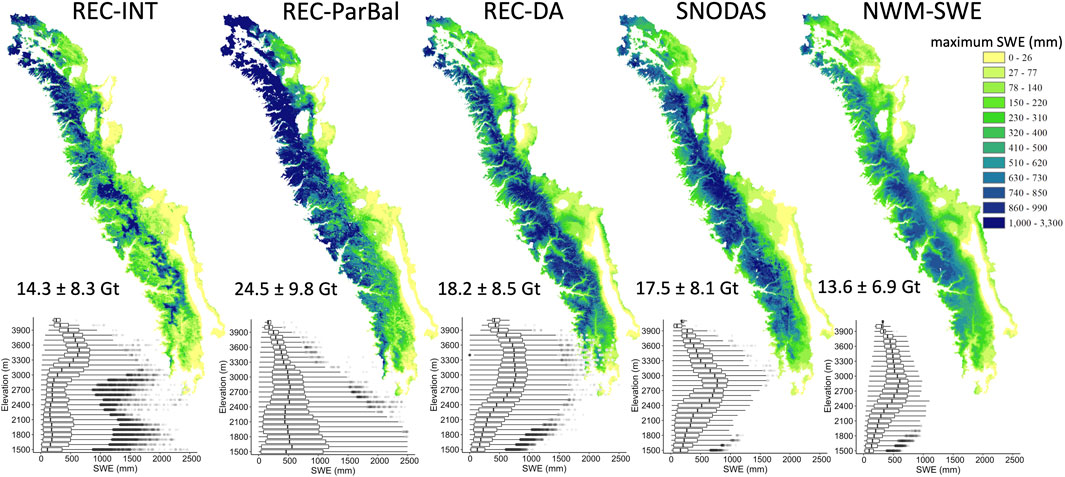
FIGURE 11. The spatial distribution of the 11-year average pixel-wise maximum SWE for the five SWE datasets in comparison across the study domain. The 11-year average and one standard deviation of maximum SWS are labeled at the bottom left for each dataset with the elevational distribution represented by the boxplot. Gt stands for gigaton, equivalent to 1 km3 of water.
The spatial distributions of maximum SWE for the two reconstructed SWE datasets (i.e., REC-INT and REC-ParBal) also exhibited similarity. Both datasets showed high maximum SWE in the NW and low maximum SWE for most other regions. However, the overall maximum SWS for REC-ParBal was much higher than REC-INT. REC-ParBal had the highest 11-year average maximum SWE, reporting 24.5 ± 9.8 Gt maximum SWS, while REC-INT had a small SWS (14.3 ± 8.3 Gt). Additionally, REC-ParBal estimated greater maximum SWE at elevations below 2,400 m where most of the area is, particularly for the western Sierra.
This study provided a comprehensive evaluation and inter-comparison of five SWE datasets at annual, seasonal, and regional scales using multiple independent validation datasets in the Sierra Nevada, California. Through the validation, this study indicated that REC-DA exhibited the highest accuracy among all five SWE data products, followed by REC-ParBal. REC-INT and SNODAS showed comparable accuracy, and NWM-SWE was the least accurate of the five datasets. The major findings of this study will guide to the use of these SWE datasets as well as contribute to future improvement of SWE estimation approaches. Below we provide a thorough discussion regarding 1) the impacts of forest canopies on retrospective SWE estimation approaches, 2) the applications of real-time SWE datasets, and 3) the utility of retrospective SWE in improving real-time SWE modeling.
Uncertainty in SWE estimation approaches can be introduced via many factors, such as the radiative and turbulent flux calculations in physically based models, detection of snow disappearance date from satellite observations, model parameterizations, and model structural assumptions, and for forward-type models, precipitation forcings. Identifying the dominant sources of uncertainty for each of the models compared herein is challenging and is outside the scope of this study. However, the pronounced differences in model results in forested regions indicate that a discussion about the influence of canopy cover adjustment on the performance of the three reconstructed SWE datasets in forested regions is warranted.
Estimating SWE under forest canopies is more challenging than estimating SWE in open areas (Rutter et al., 2009). These challenges were evident in the REC-DA, REC-INT, and REC-ParBal results whereby relatively poor performance was evident in forested regions among three land cover types (Tables 4, 6) given the difficulties in observing under canopy snow cover from satellite (Raleigh et al., 2013; Rittger et al., 2020) and complications associated with the impact of snow-vegetation interactions on model calculations of snow-atmosphere energy exchange, especially solar (Musselman et al., 2013) and longwave radiation (Musselman and Pomeroy, 2017). Efforts have been made to improve SWE modeling by improving snow cover estimation in forested regions (Liu et al., 2004; Arslan et al., 2017; Wang X. et al., 2018; De Gregorio et al., 2019; Rittger et al., 2020; Tong et al., 2020). Because the under-canopy snow cover cannot be observed directly by optical satellite imagery, REC- INT used a viewable gap fraction approach to estimate under canopy snow cover, in which the fractional snow-covered area (FSCA) value for each pixel is equivalent to the observed FSCA divided by the fraction of the pixel that does not contain vegetation (Guan et al., 2013). In the comparison between canopy-adjusted MODIS-derived FSCA and ground-based FSCA, Raleigh et al. (2013) showed that MODIS FSCA underestimation may range from 9% to 22% at meadow sites, and from 9% to 37% at forested sites during the snowmelt season. The underestimation of FSCA may potentially lead to a significant underestimation of SWE within the REC-INT model given the crude representation of viewable gap fraction in REC-INT versus REC-ParBal.
REC-ParBal used a viewing zenith angle dependent canopy adjustment approach to estimate under canopy snow cover, which accounts for off-nadir effects of wide-swath satellites (Rittger et al., 2020). In addition to the viewable gap fraction adjustment in forested regions, the viewing angle of satellite observations has significant impacts on the estimations of viewable FSCA and canopy density and thus significantly influences canopy adjustments to FSCA estimates (Liu et al., 2004; Rittger et al., 2020). For example, the viewing zenith angles for wide-swath sensors such as MODIS, used both in REC-INT and REC-ParBal, increase with off-nadir overpasses resulting in stretched pixels and obscured observations (Liu et al., 2004; Margulis et al., 2019; Rittger et al., 2020). In this context, Rittger et al. (2020) developed a viewing zenith angle dependent canopy adjustment approach to reduce the influence of oblique viewing angles on MODIS FSCA estimates; FSCA biases in forested regions decreased by 20% (Rittger et al., 2020). This adjustment could be one reason that REC-ParBal showed much better performance than REC-INT in forested regions in the TRB. We compared this snow cover adjustment method to another spectral mixture approach called SPIReS (Snow Property Inversion From Remote Sensing, Bair et al., 2019) that uses the Geometric Optical model (Liu et al., 2004) and it showed similar snow cover in forested regions. Furthermore, recent validation work with ASO-based 3-m resolution snow cover estimates show relatively stable RMSE and bias with increasing canopy fraction (Stillinger et al., 2023). However, the viewing zenith angle dependent canopy adjustment approach is likely to have over-adjusted FSCA in very dense forested regions, such as the NE Sierra where REC-ParBal estimated much higher April SWE than all other SWE datasets.
The viewable gap fraction and viewing zenith angle dependent canopy adjustment methods mentioned above both assume that the viewable FSCA under forest canopies is proportional to FSCA in open areas (Liu et al., 2004; Durand et al., 2008b; Molotch & Margulis, 2008; Rittger et al., 2020). This assumption is, however, not always true given the complexities of snow-vegetation interactions. For example, during the snow accumulation period, snowfall interception by tree canopies decreases snow accumulation under the canopy (Pomeroy et al., 1993). During the snowmelt period, canopy cover has a significant influence on the snow energy balance by changing both radiative and turbulent fluxes (Dozier, 1980; Rutter et al., 2009). Importantly, REC-DA did not use the viewable gap fraction or viewing zenith angle approach to estimate under-canopy snow cover. Instead, the particle batch smoother method used in REC-DA only updated the prior FSCA predictions for open (canopy-free) fractions of a pixel. Updates to the precipitation estimates within the REC-DA framework, therefore, were applied over open areas, with canopy adjustments then applied to predict SWE for the canopy-covered fraction of a pixel (Girotto et al., 2014a). Unlike REC-INT and REC-ParBal which treated FSCA as error free, this updating process also accounted for the uncertainties in FSCA observations. While many other improvements in REC-DA have been documented in earlier studies (Girotto et al., 2014a; 2014b; Margulis et al., 2015; 2016), the advantage of the canopy adjustment scheme and accounting for FSCA uncertainties are two potential reasons that REC-DA performed better than REC-INT and REC-ParBal in forested regions (Girotto et al., 2014b).
Among five SWE datasets compared in the study, only SNODAS and NWM are capable to provide real-time SWE estimates, though they showed much lower accuracy than the other three reconstructed SWE datasets. While SNODAS has been used in several water balance (e.g., Santner et al., 2003; Wang J. et al., 2018; Cao et al., 2019) and hydrological modeling studies (Barlage et al., 2010; Boyle et al., 2013; Massmann, 2019), a well-documented evaluation of SNODAS model performance is largely absent in the literature. Clow et al. (2012) compared snow depth and SWE estimates from SNODAS with ground snow survey measurements in Colorado and found that SNODAS SWE estimates only explained 30% of the variance in SWE in alpine environments but performed much better in forested regions, explaining 77% of the variance in observed SWE. Hedrick et al. (2015) showed that SNODAS underestimated snow depth over dense coniferous forested regions. Bair et al. (2016) also compared SNODAS SWE with ASO SWE data but found a consistent SWE underestimation, possibly because of the shorter period used in their study (i.e., 3-years were compared from 2013 to 2015) but also possibly because some mountain regions lack nearby snow pillows.
By comparing with multi-source validation datasets covering a wide range of climatic conditions and topographic characteristics, this study found the performance of SNODAS SWE estimates varied spatially and temporally, and thus are consistent with the diverse findings in previous studies (Clow et al., 2012; Hedrick et al., 2015; Bair et al., 2016). We also showed that SNODAS overestimated SWE in forested regions but underestimated SWE for a few isolated alpine areas, which corresponds with the Lv and Pomeroy (2020) evaluation in the Marmot Creek Research Basin in the Front Range of the Canadian Rockies. They also found SNODAS overestimated SWE in needle-leaf forested regions and showed that the lack of detail in snow-forest interactions within the SNODAS model reduced model accuracy in sub-canopy environments.
The NWM-SWE relies on a land surface model (Noah-MP) to estimate SWE (Niu et al., 2011; Yang et al., 2011). The NWM has a three-layer snow model with improved representations of ground heat flux, retention, percolation, and refreezing and melted liquid water within the multilayer snowpack (Yang et al., 2011). Interestingly, NWM-SWE’s performance in forested regions showed a 12.6% positive bias, which may be related to the separation of the vegetation canopy from the snow surface regarding model calculations of energy and water fluxes (Niu et al., 2011; Yang et al., 2011). However, just like many other large-scale SWE datasets (Wrzesien et al., 2019), NWM-SWE exhibited significant SWE underestimation, particularly at high elevations.
We show that the retrospective approaches (REC-INT, REC-ParBal, and REC-DA) could yield SWE estimates with accuracy levels much higher than the real-time SWE estimates other than ASO, perhaps not a surprising result given the additional information available to retrospective models. Because the spatial patterns of SWE show high similarity from year to year due to the relatively constant environmental control factors over time (e.g., topography, vegetation, and weather) (Sturm and Wagner, 2010), one important application of retrospective SWE datasets is to inform real-time SWE estimation approaches with more accurate historical SWE patterns. Early studies have explored the performance of integrating SWE patterns from reconstruction models into real-time snowpack estimation models (Schneider and Molotch, 2016; Bair et al., 2018; Zheng et al., 2018; Yang et al., 2022). Schneider and Molotch, (2016) showed a significant model improvement with a 97% (24.7%) decrease in PBIAS, and an 8% (20 mm) decrease in RMSE by integrating historical SWE patterns from REC-INT into a real-time SWE estimation model over the upper Colorado River Basin, which has been further improved by ingesting REC-DA (Yang et al., 2022). Notably, the use of real-time snow cover estimates in National Weather Service-like forecasts along with snow pillow SWE result in an 80% average improvement in forecast skill (Micheletty et al., 2021). Zheng et al. (2018) used historical SWE estimates (i.e., REC-INT) to aid in the interpolation of SWE measurements using a k-nearest neighbors algorithm and found that the spatial accuracy of the historical data is more important than the amount of data within the archive. Bair et al. (2016) used machine learning techniques to integrate historical SWE patterns from REC-ParBal to estimate SWE over the Hindu Kush, Afghanistan and found the approach provided reasonable SWE estimates with 0%–14% bias and 46–48 mm RMSE overall. Hence, given the previous supportive findings (Schneider & Molotch, 2016; Bair et al., 2018; Zheng et al., 2018), as well as the significantly better performance of the SWE reanalysis (REC-DA) and SWE reconstruction models (REC-ParBal and REC-INT) compared with the operational data products (SNODAS and NWM-SWE), this study highlights the potential applications for applying the SWE patterns from SWE reanalysis or SWE reconstructions in a variety of Earth Science applications.
To include the two reconstruction SWE datasets (REC-INT and REC-ParBal), we limited our evaluation to the snow melt season, which is one of the limitations of our study, and thus the conclusions may not represent model accuracy for other parts of the snow seasons such as the fall and winter snow accumulation period. Future work is needed to provide a more thorough evaluation of the three SWE datasets (REC-DA, SNODAS, and NWM-SWE) that are available for the entire snow season. Additionally, although we included both in situ and ASO SWE in the data evaluation, neither dataset offers ground-truth SWE at a 500 m grid cell scale. For example, the ASO SWE uncertainty is non-negligible and requires further quantification, while the in situ observations likely lack representativeness when scaled to grid cells. Lastly, given that ASO data are only recently available and limited to a few basins, the validation may not adequately capture all snow conditions and locations. Nevertheless, the study provides the most comprehensive intercomparison of these datasets to date and provides useful first-order estimates on their likely SWE errors.
This study uses three independent validation datasets to systematically evaluate the five state-of-the-art SWE data products in the Sierra Nevada, California at annual, seasonal, and regional scales, and discusses the SWE data accuracy in forests, alpine, and other open areas. The SWE datasets include two reconstruction SWE products (REC-INT, REC-ParBal), a Bayesian reanalysis product (REC-DA), and two operational SWE products (SNODAS and NWM-SWE). The results show that REC-DA consistently exhibits the best performance in capturing the spatial distribution of SWE at the pixel scale (R2 = 0.87, MAE = 66 mm, PBIAS = 8.3%), while REC-Parbal has the least overall PBIAS (R2 = 0.79, MAE = 73 mm, PBIAS = 4.1%) in the snowmelt season. When comparing maximum SWE at snow pillow stations across the Sierra Nevada, REC-DA underestimated peak SWE by −5.8%, while REC-ParBal overestimated it by 7.5%. The other SWE products—SNODAS, REC-INT, and NWM-SWE—are less accurate. The inter-model comparison suggested a certain amount of disagreement of snow water resources between SWE datasets across time and space in the Sierra Nevada. From the 11-year record, REC-ParBal overall had the highest 1 April SWE bolstered by large volumes at moderate elevations with large areas, which is 27%, 22%, 29%, and 43% greater than REC-INT, REC-DA, SNODAS, and NWM-SWE, respectively. REC-INT and REC-ParBal exhibited higher amounts of 1 April SWS than the other three datasets at lower elevations where there is more forest. The average maximum snow water storage (SWS) for the study domain was 17.6 Gt, ranging from 13.6 Gt estimated by NWM-SWE to 24.5 Gt estimated by REC-ParBal. This critical validation and inter-model comparison of different SWE datasets across a large mountainous region helps to improve our understanding of SWE estimation uncertainties. Given the importance of these mountainous regions for sustaining water supplies, the results of this study have broad implications for water resource management and for process-based hydrological studies.
The datasets presented in this study can be found in online repositories. The names of the repository/repositories and accession number(s) can be found in the article/Supplementary Material.
KY: Conceptualization, Methodology, Validation, Software, Writing—Original Draft, Review and Editing, Visualization; KR: Resources, Writing—Review and Editing; KM: Conceptualization, Writing—Review and Editing; EB: Resources, Writing—Review and Editing; JD: Conceptualization, Writing—Review and Editing; SM: Resources, Writing—Review and Editing; TP: Resources, Writing—Review and Editing; NM: Conceptualization, Methodology, Validation, Supervision, Funding acquisition, Writing—Original Draft, Review and Editing. All authors contributed to the article and approved the submitted version.
This study was supported by the NASA grants NNX17AF50G (Analysis of Agricultural Water Supply-Demand Imbalance During the Unprecedented California Drought Using NASA Satellite Data), NASA 80NSSC18K0427 P00001 (Near Real Time Snow Analyses). The gap filled FSCA and REC-ParBal SWE data was supported by NASA 80NSSC18K0427, 80NSSC22K0703, 80NSSC22K0929, 80NSSC18K1489, 80NSSC20K1349, and NOAA NA18OAR4590367.
The authors declare that the research was conducted in the absence of any commercial or financial relationships that could be construed as a potential conflict of interest.
All claims expressed in this article are solely those of the authors and do not necessarily represent those of their affiliated organizations, or those of the publisher, the editors and the reviewers. Any product that may be evaluated in this article, or claim that may be made by its manufacturer, is not guaranteed or endorsed by the publisher.
The Supplementary Material for this article can be found online at: https://www.frontiersin.org/articles/10.3389/feart.2023.1106621/full#supplementary-material
Arslan, A. N., Tanis, C. M., Metsämäki, S., Aurela, M., Böttcher, K., Linkosalmi, M., et al. (2017). Automated webcam monitoring of fractional snow cover in northern boreal conditions. Geosciences, 7, (3), 55. doi:10.3390/GEOSCIENCES7030055
Bair, E. H., Calfa, A. A., Rittger, K., and Dozier, J. (2018). Using machine learning for real-time estimates of snow water equivalent in the watersheds of Afghanistan. Cryosphere 12 (5), 1579–1594. doi:10.5194/tc-12-1579-2018
Bair, E. H., Rittger, K., Davis, R. E., Painter, T. H., and Dozier, J. (2016). Validating reconstruction of snow water equivalent in California’s Sierra Nevada using measurements from the NASA Airborne Snow Observatory. Water Resour. Res. 52 (11), 8437–8460. doi:10.1002/2016WR018704
Bair, E. H., Rittger, K., Skiles, S. M., and Dozier, J. (2019). An examination of snow albedo estimates from MODIS and their impact on snow water equivalent reconstruction. Water Resour. Res. 55 (9), 7826–7842. doi:10.1029/2019WR024810
Bales, R. C., Molotch, N. P., Painter, T. H., Dettinger, M. D., Rice, R., and Dozier, J. (2006). Mountain hydrology of the Western United States. Water Resour. Res. 42 (8), W08432. doi:10.1029/2005WR004387
Balk, B., and Elder, K. (2000). Combining binary decision tree and geostatistical methods to estimate snow distribution in a mountain watershed. Water Resour. Res. 36 (1), 13–26. doi:10.1029/1999WR900251
Barlage, M., Chen, F., Tewari, M., Ikeda, K., Gochis, D., Dudhia, J., et al. (2010). Noah land surface model modifications to improve snowpack prediction in the Colorado Rocky Mountains. J. Geophys. Res. 115, D22101. doi:10.1029/2009JD013470
Barrett, A. P. (2003). National operational hydrologic remote sensing center snow data assimilation system (SNODAS) products at NSIDC. NSIDC Spec. Rep. 11. doi:10.7265/N5TB14TC
Bormann, K. J., Hedrick, A., Patterson, V. M., Deems, J. S., Marks, D., and Painter, T. H. (2018). Per-pixel uncertainty for the airborne snow observatory’s SWE products. Washington, D.C: American Geophysical Union Falling Meeting.
Boyle, D., Barth, C., and Bassett, S. (2013). “Towards improved hydrologic model predictions in ungauged snow-dominated watersheds utilizing a multi-criteria approach and SNODAS estimates of SWE,” in Putting prediction in ungauged basins into practice (Canada: Canadian Water Resources Association), 231–242.
Cao, Q., Clark, E. A., Mao, Y., and Lettenmaier, D. P. (2019). Trends and interannual variability in terrestrial water storage over the eastern United States, 2003–2016. Water Resour. Res. 55 (3), 1928–1950. doi:10.1029/2018WR023278
Carroll, T., Cline, D., Fall, G., Nilsson, A., Li, L., and Rost, A. (2001). “NOHRSC operations and the simulation of snow cover properties for the coterminous U.S,” in Proceedings of the 69th Annual meeting of the Western Snow Conference, Sun Valley, Idaho, April 2001, 1–14.
Cline, D. W., Bales, R. C., and Dozier, J. (1998). Estimating the spatial distribution of snow in mountain basins using remote sensing and energy balance modeling. Water Resour. Res. 34 (5), 1275–1285. doi:10.1029/97wr03755
Clow, D. W., Nanus, L., Verdin, K. L., and Schmidt, J. (2012). Evaluation of SNODAS snow depth and snow water equivalent estimates for the Colorado Rocky Mountains, USA. Hydrol. Process. 26 (17), 2583–2591. doi:10.1002/hyp.9385
Cornwell, E., Molotch, N. P., and McPhee, J. (2016). Spatio-temporal variability of snow water equivalent in the extra-tropical Andes Cordillera from distributed energy balance modeling and remotely sensed snow cover. Hydrology Earth Syst. Sci. 20 (1), 411–430. doi:10.5194/hess-20-411-2016
Cortés, G., Girotto, M., and Margulis, S. A. (2014). Analysis of sub-pixel snow and ice extent over the extratropical Andes using spectral unmixing of historical Landsat imagery. Remote Sens. Environ. 141, 64–78. doi:10.1016/j.rse.2013.10.023
Daly, C., Neilson, R. P., and Phillips, D. L. (1994). A statistical-topographic model for mapping climatological precipitation over mountainous terrain. J. Appl. Meteorology 33 (2), 140–158. doi:10.1175/1520-0450(1994)033<0140:ASTMFM>2.0.CO;2
De Gregorio, L., Callegari, M., Marin, C., Zebisch, M., Bruzzone, L., Demir, B., et al. (2019). A novel data fusion technique for snow cover retrieval. IEEE J. Sel. Top. Appl. Earth Observations Remote Sens. 12 (8), 2862–2877. doi:10.1109/JSTARS.2019.2920676
DeWalle, D. R., and Rango, A. (2008). Principles of snow hydrology. Cambridge: Cambridge University Press. doi:10.1017/CBO9780511535673
Dozier, J. (1980). A clear-sky spectral solar radiation model for snow-covered mountainous terrain. Water Resour. Res. 16 (4), 709–718. doi:10.1029/WR016i004p00709
Dozier, J., Bair, E. H., and Davis, R. E. (2016). Estimating the spatial distribution of snow water equivalent in the world’s mountains. Wiley Interdiscip. Rev. Water 3 (3), 461–474. doi:10.1002/wat2.1140
Durand, M., Molotch, N. P., and Margulis, S. A. (2008a). A Bayesian approach to snow water equivalent reconstruction. J. Geophys. Res. 113, D20117. doi:10.1029/2008JD009894
Durand, M., Molotch, N. P., and Margulis, S. A. (2008b). Merging complementary remote sensing datasets in the context of snow water equivalent reconstruction. Remote Sens. Environ. 112 (3), 1212–1225. doi:10.1016/j.rse.2007.08.010
Erxleben, J., Elder, K., and Davis, R. (2002). Comparison of spatial interpolation methods for estimating snow distribution in the Colorado Rocky Mountains. Hydrol. Process. 16 (18), 3627–3649. doi:10.1002/hyp.1239
Fang, Y., Liu, Y., and Margulis, S. A. (2022). A Western United States snow reanalysis dataset over the Landsat era from water years 1985 to 2021. Sci. Data 9, 677. doi:10.1038/s41597-022-01768-7
Girotto, M., Cortés, G., Margulis, S. A., and Durand, M. (2014a). Examining spatial and temporal variability in snow water equivalent using a 27 year reanalysis: Kern River watershed, Sierra Nevada. Water Resour. Res. 50 (8), 6713–6734. doi:10.1002/2014WR015346
Girotto, M., Margulis, S. A., and Durand, M. (2014b). Probabilistic SWE reanalysis as a generalization of deterministic SWE reconstruction techniques. Hydrol. Process. 28 (12), 3875–3895. doi:10.1002/hyp.9887
Gochis, D. J., Barlage, M., Dugger, A., FitzGerald, K., Karsten, L., McAllister, M., et al. (2018). The WRF-Hydro modeling system technical description. Version 5.0. Boulder, Colorado: NCAR Technical Note.
Guan, B., Molotch, N. P., Waliser, D. E., Jepsen, S. M., Painter, T. H., and Dozier, J. (2013). Snow water equivalent in the Sierra Nevada: Blending snow sensor observations with snowmelt model simulations. Water Resour. Res. 49 (8), 5029–5046. doi:10.1002/wrcr.20387
Hansen, M. C., Potapov, P. V., Moore, R., Hancher, M., Turubanova, S. A., Tyukavina, A., et al. (2013). High-resolution global maps of 21st-century forest cover change. Science 342 (6160), 850–853. doi:10.1126/science.1244693
Hedrick, A., Marshall, H.-P., Winstral, A., Elder, K., Yueh, S., and Cline, D. (2015). Independent evaluation of the SNODAS snow depth product using regional-scale lidar-derived measurements. Cryosphere 9 (1), 13–23. doi:10.5194/tc-9-13-2015
Huning, L. S., and AghaKouchak, A. (2018). Mountain snowpack response to different levels of warming. Proc. Natl. Acad. Sci. 115 (43), 10932–10937. doi:10.1073/pnas.1805953115
Jennings, K. S., Kittel, T. G. F., and Molotch, N. P. (2018). Observations and simulations of the seasonal evolution of snowpack cold content and its relation to snowmelt and the snowpack energy budget. Cryosphere 12 (5), 1595–1614. doi:10.5194/tc-12-1595-2018
Jepsen, S. M., Molotch, N. P., Williams, M. W., Rittger, K. E., and Sickman, J. O. (2012). Interannual variability of snowmelt in the Sierra Nevada and Rocky Mountains, United States: Examples from two alpine watersheds. Water Resour. Res. 48 (2). doi:10.1029/2011WR011006
Liston, G. E. (2004). Representing subgrid snow cover heterogeneities in regional and global models. J. Clim. 17 (6), 1381–1397. doi:10.1175/1520-0442(2004)017<1381:RSSCHI>2.0.CO;2
Liu, J., Melloh, R. A., Woodcock, C. E., Davis, R. E., and Ochs, E. S. (2004). The effect of viewing geometry and topography on viewable gap fractions through forest canopies. Hydrol. Process. 18 (18), 3595–3607. doi:10.1002/HYP.5802
Lopez-Moreno, J. I., Fassnacht, S. R., Heath, J. T., Musselman, K. N., Revuelto, J., La- tron, J., et al. (2013). Small scale spatial variability of snow density and depth over complex alpine terrain: Implications for estimating snow water equivalent. Adv. Water Resour. 55, 40–52. doi:10.1016/j.advwatres.2012.08.010
Lv, Z., and Pomeroy, J. W. (2020). Assimilating snow observations to snow interception process simulations. Hydrol. Process. 34 (10), 2229–2246. doi:10.1002/hyp.13720
Margulis, S. A., Cortés, G., Girotto, M., and Durand, M. (2016). A landsat-era Sierra Nevada snow reanalysis (1985–2015). J. Hydrometeorol. 17 (4), 1203–1221. doi:10.1175/JHM-D-15-0177.1
Margulis, S. A., Girotto, M., Cortés, G., and Durand, M. (2015). A particle batch smoother approach to snow water equivalent estimation. J. Hydrometeorol. 16 (4), 1752–1772. doi:10.1175/JHM-D-14-0177.1
Margulis, S. A., Liu, Y., and Baldo, E. (2019). A joint Landsat and MODIS-based reanalysis approach for midlatitude montane seasonal snow characterization. Front. Earth Sci. 7, 272. doi:10.3389/feart.2019.00272
Marks, D., Domingo, J., Susong, D., Link, T., and Garen, D. (1999). A spatially distributed energy balance snowmelt model for application in mountain basins. Hydrol. Process. 13 (12–13), 1935–1959. doi:10.1002/(SICI)1099-1085(199909)13:12/13<1935::AID-HYP868>3.0.CO;2-C
Martinec, J., and Rango, A. (1981). Areal distribution of snow water equivalent evaluated by snow cover monitoring. Water Resour. Res. 17, 1480–1488. doi:10.1029/WR017i005p01480
Massmann, C. (2019). Modelling snowmelt in ungauged catchments. Water 11, 301. doi:10.3390/w11020301
Meromy, L., Molotch, N. P., Link, T. E., Fassnacht, S. R., and Rice, R. (2013). Subgrid variability of snow water equivalent at operational snow stations in the Western USA. Hydrol. Process. 27 (17), 2383–2400. doi:10.1002/hyp.9355
Meyer, C., Weiant, P., Serpa, L., Tam, C., Cox, R., and Gaither, J. (1999). Sierra Nevada ecoregional plan. The nature conservancy. Available at: http://www.conservationgateway.org/ConservationPlanning/SettingPriorities/EcoregionalReports/Documents/SierraNV_plan_LowRes.pdf (accessed April 17, 2023).
Micheletty, P., Perrot, D., Day, G., and Rittger, K. (2021). Assimilation of ground and satellite snow observations in a distributed hydrologic model for water supply forecasting. JAWRA J. Am. Water Resour. Assoc. 58, 1030–1048. doi:10.1111/1752-1688.12975
Molotch, N. P., and Bales, R. C. (2005). Scaling snow observations from the point to the grid element: Implications for observation network design. Water Resour. Res. 41 (11), W11421. doi:10.1029/2005WR004229
Molotch, N. P., and Bales, R. C. (2006). SNOTEL representativeness in the Rio Grande headwaters on the basis of physiographics and remotely sensed snow cover persistence. Hydrol. Process. 20 (4), 723–739. doi:10.1002/hyp.6128
Molotch, N. P., Colee, M. T., Bales, R. C., and Dozier, J. (2005). Estimating the spatial distribution of snow water equivalent in an alpine basin using binary regression tree models: The impact of digital elevation data and independent variable selection. Hydrol. Process. 19 (7), 1459–1479. doi:10.1002/hyp.5586
Molotch, N. P., Durand, M. T., Guan, B., Margulis, S. A., and Davis, R. E. (2014). “Snow cover depletion curves and snow water equivalent reconstruction,” in Remote sensing of the terrestrial water cycle (D.C., United States: American Geophysical Union AGU), 157–173. doi:10.1002/9781118872086.ch10
Molotch, N. P., and Margulis, S. A. (2008). Estimating the distribution of snow water equivalent using remotely sensed snow cover data and a spatially distributed snowmelt model: A multi-resolution, multi-sensor comparison. Adv. Water Resour. 31 (11), 1503–1514. doi:10.1016/j.advwatres.2008.07.017
Molotch, N. P. (2009). Reconstructing snow water equivalent in the Rio Grande headwaters using remotely sensed snow cover data and a spatially distributed snowmelt model. Hydrol. Process. 23 (7), 1076–1089. doi:10.1002/hyp.7206
Musselman, K. N., Margulis, S. A., and Molotch, N. P. (2013). Estimation of solar direct beam transmittance of conifer canopies from airborne LiDAR. Remote Sens. Environ. 136, 402–415. doi:10.1016/j.rse.2013.05.021
Musselman, K. N., and Pomeroy, J. W. (2017). Estimation of needleleaf canopy and trunk temperatures and longwave contribution to melting snow. J. Hydrometeorol. 18 (2), 555–572. doi:10.1175/JHM-D-16-0111.1
Niu, G.-Y., Yang, Z.-L., Mitchell, K. E., Chen, F., Ek, M. B., Barlage, M., et al. (2011). The community Noah land surface model with multiparameterization options (Noah-MP): 1. Model description and evaluation with local-scale measurements. J. Geophys. Res. 116, D12109. doi:10.1029/2010JD015139
Painter, T. H., Berisford, D. F., Boardman, J. W., Bormann, K. J., Deems, J. S., Gehrke, F., et al. (2016). The Airborne Snow Observatory: Fusion of scanning lidar, imaging spectrometer, and physically-based modeling for mapping snow water equivalent and snow albedo. Remote Sens. Environ. 184, 139–152. doi:10.1016/j.rse.2016.06.018
Painter, T. H., Rittger, K., McKenzie, C., Slaughter, P., Davis, R. E., and Dozier, J. (2009). Retrieval of subpixel snow covered area, grain size, and albedo from MODIS. Remote Sens. Environ. 113 (4), 868–879. doi:10.1016/j.rse.2009.01.001
Pomeroy, J. W., Gray, D. M., and Landine, P. G. (1993). The prairie blowing snow model: Characteristics, validation, operation. J. Hydrology 144 (1–4), 165–192. doi:10.1016/0022-1694(93)90171-5
Raleigh, M. S., and Lundquist, J. D. (2012). Comparing and combining SWE estimates from the SNOW-17 model using PRISM and SWE reconstruction. Water Resour. Res. 48 (1), W01506. doi:10.1029/2011WR010542
Raleigh, M. S., Rittger, K., Moore, C. E., Henn, B., Lutz, J. A., and Lundquist, J. D. (2013). Ground-based testing of MODIS fractional snow cover in subalpine meadows and forests of the Sierra Nevada. Remote Sens. Environ. 128, 44–57. doi:10.1016/j.rse.2012.09.016
Rittger, K., Bair, E. H., Kahl, A., and Dozier, J. (2016). Spatial estimates of snow water equivalent from reconstruction. Adv. water Resour. 94, 345–363. doi:10.1016/j.advwatres.2016.05.015
Rittger, K., Raleigh, M. S., Dozier, J., Hill, A. F., Lutz, J. A., and Painter, T. H. (2020). Canopy adjustment and improved cloud detection for remotely sensed snow cover mapping. Water Resour. Res. 56 (6), 2019WR024914. doi:10.1029/2019WR024914
Rutter, N., Essery, R., Pomeroy, J., Altimir, N., Andreadis, K., Baker, I., et al. (2009). Evaluation of forest snow processes models (SnowMIP2). J. Geophys. Res. 114 (D6), D06111. doi:10.1029/2008JD011063
Santner, T. J., Williams, B. J., Notz, W. I., and Williams, B. J. (2003). The design and analysis of computer experiments. Heidelberg, Germany: Springer.
Schneider, D., and Molotch, N. P. (2016). Real-time estimation of snow water equivalent in the Upper Colorado River Basin using MODIS-based SWE Reconstructions and SNOTEL data. Water Resour. Res. 52 (10), 7892–7910. doi:10.1002/2016WR019067
Slater, A. G., Barrett, A. P., Clark, M. P., Lundquist, J. D., and Raleigh, M. S. (2013). Uncertainty in seasonal snow reconstruction: Relative impacts of model forcing and image availability. Adv. Water Resour. 55, 165–177. doi:10.1016/j.advwatres.2012.07.006
Snow Today (2022). Nsidc. Available at: https://nsidc.org/reports/snow-today (Accessed July 6, 2022).
Stillinger, T., Rittger, K., Raleigh, M. S., Michell, A., Davis, R. E., and Bair, E. H. (2023). Landsat, MODIS, and VIIRS snow cover mapping algorithm performance as validated by airborne lidar datasets. Cryosphere 17, 567–590. doi:10.5194/tc-17-567-2023
Sturm, M., and Wagner, A. M. (2010). Using repeated patterns in snow distribution modeling: An Arctic example. Water Resour. Res. 46 (12), 1–15. doi:10.1029/2010WR009434
Swain, D. L., Horton, D. E., Singh, D., and Diffenbaugh, N. S. (2016). Trends in atmospheric patterns conducive to seasonal precipitation and temperature extremes in California. Sci. Adv. 2 (4), e1501344. doi:10.1126/sciadv.1501344
Taylor, K. E. (2001). Summarizing multiple aspects of model performance in a single diagram. J. Geophys. Res. Atmos. 106, 7183–7192. doi:10.1029/2000JD900719
Tong, R., Parajka, J., Komma, J., and Blöschl, G. (2020). Mapping snow cover from daily Collection 6 MODIS products over Austria. J. Hydrology 590, 125548. doi:10.1016/J.JHYDROL.2020.125548
Trujillo, E., Molotch, N. P., Goulden, M. L., Kelly, A. E., and Bales, R. C. (2012). Elevation-dependent influence of snow accumulation on forest greening. Nat. Geosci. 5 (10), 705–709. doi:10.1038/ngeo1571
Wang, J., Song, C., Reager, J. T., Yao, F., Famiglietti, J. S., Sheng, Y., et al. (2018a). Recent global decline in endorheic basin water storages. Nat. Geosci. 11 (12), 926–932. doi:10.1038/s41561-018-0265-7
Wang, X., Wang, J., Che, T., Huang, X., Hao, X., and Li, H. (2018b). Snow cover mapping for complex mountainous forested environments based on a multi-index technique. IEEE J. Sel. Top. Appl. Earth Observations Remote Sens. 11 (5), 1433–1441. doi:10.1109/JSTARS.2018.2810094
Wrzesien, M. L., Pavelsky, T. M., Durand, M. T., Dozier, J., and Lundquist, J. D. (2019). Characterizing biases in mountain snow accumulation from global data sets. Water Resour. Res. 55 (11), 9873–9891. doi:10.1029/2019WR025350
Xia, Y., Mitchell, K., Ek, M., Cosgrove, B., Sheffield, J., Luo, L., et al. (2012a). Continental-scale water and energy flux analysis and validation for North American land data assimilation system project phase 2 (NLDAS-2): 2. Validation of model-simulated streamflow: Validation of model-simulated streamflow. J. Geophys. Res. 117. doi:10.1029/2011JD016051
Xia, Y., Mitchell, K., Ek, M., Sheffield, J., Cosgrove, B., Wood, E., et al. (2012b). Continental-scale water and energy flux analysis and validation for the North American land data assimilation system project phase 2 (NLDAS-2): 1. Intercomparison and application of model products: Water and energy flux analysis. J. Geophys. Res. 117. doi:10.1029/2011JD016048
Xue, Y., Sun, S., Kahan, D. S., and Jiao, Y. (2003). Impact of parameterizations in snow physics and interface processes on the simulation of snow cover and runoff at several cold region sites. J. Geophys. Res. Atmos. 108, 2002JD003174. doi:10.1029/2002JD003174
Yang, K., Musselman, K. N., Rittger, K., Margulis, S. A., Painter, T. H., and Molotch, N. P. (2022). Combining ground-based and remotely sensed snow data in a linear regression model for real-time estimation of snow water equivalent. Adv. Water Resour. 160, 104075. doi:10.1016/j.advwatres.2021.104075
Yang, Z.-L., Niu, G.-Y., Mitchell, K. E., Chen, F., Ek, M. B., Barlage, M., et al. (2011). The community Noah land surface model with multiparameterization options (Noah-MP): 2. Evaluation over global river basins. J. Geophys. Res. 116, D12110. doi:10.1029/2010JD015140
Keywords: snow water equivalent, data evaluation, airborne remote sensing, mountain snowpack, water availability
Citation: Yang K, Rittger K, Musselman KN, Bair EH, Dozier J, Margulis SA, Painter TH and Molotch NP (2023) Intercomparison of snow water equivalent products in the Sierra Nevada California using airborne snow observatory data and ground observations. Front. Earth Sci. 11:1106621. doi: 10.3389/feart.2023.1106621
Received: 24 November 2022; Accepted: 26 May 2023;
Published: 22 June 2023.
Edited by:
Patrick Alexander, Columbia University, United StatesReviewed by:
Zoe Courville, Cold Regions Research and Engineering Laboratory, United StatesCopyright © 2023 Yang, Rittger, Musselman, Bair, Dozier, Margulis, Painter and Molotch. This is an open-access article distributed under the terms of the Creative Commons Attribution License (CC BY). The use, distribution or reproduction in other forums is permitted, provided the original author(s) and the copyright owner(s) are credited and that the original publication in this journal is cited, in accordance with accepted academic practice. No use, distribution or reproduction is permitted which does not comply with these terms.
*Correspondence: Kehan Yang, a3lhbmczM0B1dy5lZHU=
Disclaimer: All claims expressed in this article are solely those of the authors and do not necessarily represent those of their affiliated organizations, or those of the publisher, the editors and the reviewers. Any product that may be evaluated in this article or claim that may be made by its manufacturer is not guaranteed or endorsed by the publisher.
Research integrity at Frontiers
Learn more about the work of our research integrity team to safeguard the quality of each article we publish.