Multichannel seismic impedance inversion based on Attention U-Net

Recently, seismic inversion has made extensive use of supervised learning methods. The traditional deep learning inversion network can utilize the temporal correlation in the vertical direction. Still, it does not consider the spatial correlation in the horizontal direction of seismic data. Each seismic trace is inverted independently, which leads to noise and large geological variations in seismic data, thus leading to lateral discontinuity. Given this, the proposed method uses the spatial correlation of the seismic data in the horizontal direction. In the network training stage, several seismic traces centered on the well-side trace and the corresponding logging curve form a set of training sample pairs for training, to enhance the lateral continuity and anti-noise performance. Additionally, Attention U-Net is introduced in acoustic impedance inversion. Attention U-Net adds attention gate (AG) model to the skip connection between the encoding and decoding layers of the U-Net network, which can give different weights to different features, so the model can focus on the features related to the inversion task and avoid the influence of irrelevant data and noise during the inversion process. The performance of the proposed method is evaluated using the Marmousi2 model and the SEAM model and compared with other methods. The experimental results show that the proposed method has the advantages of high accuracy of acoustic impedance value inversion, good transverse continuity of inversion results, and strong anti-noise performance.

1 Introduction

Seismic inversion can be defined as the process of obtaining subsurface model parameters, such as formation velocity, density, or impedance, from seismic data by comprehensively available geological and logging data (Treitel and Lines, 2001). For conventional seismic inversion methods, i.e., model-driven inversion methods, the mathematical theory is based on the convolution model or other mathematical and physical models. The convolution model is essentially a simplification and approximation of the seismic wave transmission process. The subsurface structure is usually very complex, and errors will inevitably arise when describing the wave propagation with the convolution model, which leads to inaccurate inversion results. On the other hand, in order to get a good inversion result, the model-driven method needs a better initial model and an accurate wavelet. In practical applications, it is usually challenging to obtain good initial models and accurate wavelets. In addition, problems such as limited data bandwidth, data noise, and incomplete data coverage cause various troubles for model-driven inversion methods.

Unlike traditional model-driven seismic inversion, deep learning is a data-driven approach that can learn complex non-linear mappings between inputs and outputs based on training datasets, and the parameters are adjustable. Deep learning is a subset of machine learning that has recently made breakthroughs in image classification (Krizhevsky et al., 2017), object detection (Ren et al., 2015), image segmentation (Chen et al., 2017), image and video captioning (Vinyals et al., 2022), speech recognition (Graves et al., 2013), and machine translation (Cho et al., 2014). The success of deep learning in the fields of computer vision and natural language processing has led to widespread interest among scholars in data-driven intelligent seismic inversion methods. This class of methods does not require an initial model and does not require the estimation of seismic wavelets. Using the powerful learning ability of deep neural networks to establish non-linear mapping relationships between seismic data and parameters to be inverted has become a trendy research direction in the field of seismic inversion.

Currently, the application of deep learning methods in the field of seismic inversion is expanding, involving acoustic impedance inversion, pre-stack elastic and lithological parameter inversion, full waveform inversion, and so on. Recently, seismic inversion has made extensive use of supervised learning methods. Alfarraj and AlRegib (2018) used recurrent neural networks for petrophysical parameter estimation. Das et al. (2019) and Wu et al. (2020) trained the convolutional neural networks (CNNs) to invert seismic impedance using synthetic seismic records on the earth model constrained by petrophysical relationships. The results show that the type of sediment phase and source wavelet parameters used in the training dataset affect the inversion process of the network. Mustafa et al. (2019) used the temporal convolution network (TCN) to estimate the acoustic impedance. This method not only successfully captured the long-term trend but also preserved the local patterns while overcoming the gradient disappearance problem in the inversion of recurrent neural network (RNN) and the overfitting problem in convolutional neural networks. Du et al. (2019) proposed SeisInv-ResNet for pre-stack seismic inversion to obtain p-wave impedance, s-wave impedance, and other petrophysical parameters. Aleardi and Salusti (2021) proposed an elastic pre-stack seismic inversion method based on CNN.

Although the above inversion networks based on deep learning can well utilize the temporal correlation in the vertical direction, they do not consider the spatial correlation of seismic data in the horizontal direction, and each seismic trace is inverted independently. However, in subsurface seismic profiles, adjacent traces are highly correlated. The inversion method based on trace by trace does not exploit the spatial correlation in the horizontal direction, which may lead to poor horizontal continuity of inversion results. To improve the continuity, Wu et al. (2021) proposed a 2D network-based inversion method.

Traditional CNN networks take a long time to train and need a lot of labeled data. To address these drawbacks of classical CNN networks, Ronneberger et al. (2015) proposed the U-Net network in their study of biomedical image segmentation problems. Their research shows that U-Net can reduce the need for labeled data to a certain extent while improving training efficiency. Seismic inversion also faces the problem of a small number of labels (few logging data) and a very large amount of seismic data. In view of this, Cao et al. (2022) proposed an inversion network consisting of a U-Net combined with three fully connected networks and named it the UCNN, which was used to predict elastic parameters from pre-stack seismic data. To further reduce the reliance on labeled data, they use Sequential Gaussian Co-Simulation and Elastic Distortion algorithms to generate adequate and diverse pre-stack seismic inversion datasets. Similarly, Wang et al. (2020) proposed a closed-loop CNN structure with a U-Net network as the main body to make CNN less dependent on the amount of labeled data in seismic inversion. The proposed closed-loop CNN can simulate both seismic forward and inversion processes from the training dataset.

Given the excessive and repeated extraction and utilization of similar features for each cascaded CNN structure in U-Net, this results in a significant computational effort and network parameter scale. Oktay et al. (2018) proposed the Attention Gate (AG) model and integrated it into U-Net to obtain the Attention U-Net network. The AG model can implicitly learn to emphasize prominent features that are helpful for inversion while suppressing irrelevant regions in the input data. In addition, AG is easily integrated into standard CNN architectures such as U-Net, which can reduce the computational overhead while improving the sensitivity and prediction accuracy of the network.

In conclusion, this paper proposes a multichannel acoustic impedance inversion based on Attention U-Net to address the issues with conventional deep learning inversion networks, such as poor continuity of inversion results and susceptibility to noise due to the trace-by-trace inversion method. The horizontal spatial correlation is applied to the inversion network by mapping multiple seismic traces to one logging curve. Under the supervision of limited logging data, the inversion network is trained. The training samples consist of several seismic traces centered on the well-side traces and associated well-logging curves. The inversion network simultaneously performs the duties of predicting acoustic impedance and forwarding seismic data. This paper is structured as follows: In Section 2, the theory and network structure of Attention U-Net are briefly introduced, and then the architecture of the inversion network consisting of three modules and their specific internal parameter settings are presented. In Section 3, the experimental results of the inversion of two typical seismic models (the Marmousi2 model and the SEAM model) are presented, analyzed, and discussed. The experimental results are compared with other deep learning inversion methods, and the noise immunity of the inversion network is discussed in this paper. Finally, Section 4 concludes this paper.

2 Methods

2.1 Inversion framework

Geological structures are spatially correlated. The closer the distance, the stronger the correlation, and conversely, the weaker the correlation. The correlation of seismic data is reflected in the temporal correlation in the vertical direction of seismic traces and the spatial correlation in the horizontal direction between the central trace and the adjacent traces. Based on the spatiotemporal characteristics of the seismic data, the inversion framework in Figure 1 is constructed using a supervised learning approach. The inversion framework shown in Figure 1 consists of three main modules: the feature extraction module, the regression module, and the forward module.

FIGURE 1

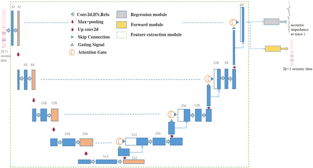
FIGURE 1. Structure of inversion network.

In the training phase, the input of the inversion network is the seismic data of the well-side trace and the 2 k nearby seismic data centered on it. The feature extraction module extracts the temporal and spatial features of the seismic data of the well-side trace and the 2 k nearby seismic traces by Attention U-Net. The regression module is used to map the data from the feature domain (spatiotemporal feature series) to the target domain (predicted acoustic impedance), while the forward module is used to map the data from the feature domain to the target domain (forward 2 k + 1 traces seismic data). Referring to the structure of the multi-task learning of Mustafa et al. (2021), the inverse network learns two tasks simultaneously: the predicted acoustic impedance data and forward seismic data. By sharing representations between the two tasks, especially if they are related to each other, we bias the network to learn more generalizable features.

2.2 Network model

2.2.1 Feature extraction module

The Attention U-Net is used as a feature extraction module to extract spatial and temporal features of seismic data. The input of the feature extraction module is the seismic data of the well-side trace and the nearby 2 k traces centered on it, and the output feature size is the same as the input size. Attention U-Net is improved by using U-Net as the base framework, as shown in Figure 1, adding AG at the jump connection between the encoding-decoding layers of the U-Net network, so that the originally up-sampled features are connected with the encoded layer AG-processed signal. By assigning different weights to different features, the model is better able to pay attention to the features relevant to the inversion task, which improves the sensitivity and prediction accuracy of the model.

Attention U-Net is divided into an encoding part and a decoding part, as shown in Figure 1. The encoding part of the Attention U-Net framework used in this paper contains four downsampling layers. The downsampling layer includes two consecutive convolutional blocks and a 2 × 1 max-pooling layer, and each convolutional block consists of a 3 × 3 two-dimensional convolutional layer (Conv2d), a batch normalization layer (BN) (Ioffe and Szegedy, 2022), and a rectified linear unit (ReLU) (Nair and Hinton, 2010) activation function. Batch normalization is used to accelerate the convergence of the network, and ReLU is used to enhance the non-linear approximation capability of the model. The decoding part corresponds to the encoding part, and the decoding part also contains four upsampling layers. Each upsampling layer consists of a 4 × 3 deconvolution layer, an AG model, and two convolution blocks.

The input of AG is the feature in the encoding part and the feature after deconvolution in the decoding part. The specific structure of AG is shown in Figure 2. The features extracted from the decoding part after deconvolution are used as the gating signal g, and the features from the matching layer’s coding portion are used as x. The 1 × 1 convolution is done for g and x, and the two results A and B are added element by element to highlight the features. Then, the non-linear ability of the added result is increased by the ReLU activation function to obtain C, and the channel of C is reduced to 1 channel by a convolution operation. D is processed using a sigmoid activation function such that its value falls within the range of (0, 1), and the result is an attention weight that is the same size as the input feature and has one channel. Finally, the attention weight is multiplied by x.

FIGURE 2

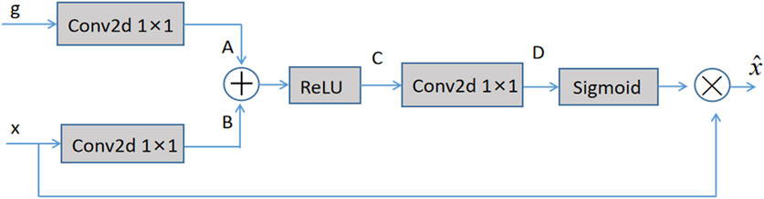
FIGURE 2. Attention gating model.

2.2.2 Regression module

The regression module maps the output of the feature extraction module from the feature domain to the target domain. The regression module’s structure, as shown in Figure 3, consists of two convolutional blocks and a 2D convolutional layer. Each convolutional block consists of a 2D convolutional layer, a group normalization layer, and the ReLU activation function. Group normalization groups the outputs of the convolutional layers and normalizes each group using the learned mean and standard deviation, which have been shown to reduce covariate bias in the learned features and speed up learning (Wu and He, 2012).

FIGURE 3

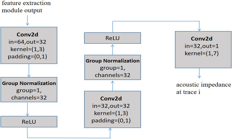
FIGURE 3. Block diagram of the regression module.

As shown in Figure 3, the input of the regression module is the output of the feature extraction module, and the output is the predicted acoustic impedance. Calculate the mean square error between the actual acoustic impedance and the output of the regression module. In other words, the mean square error between the predicted and the actual acoustic impedance data is calculated to update the learnable parameters in the feature extraction module and the regression module. The following Eq. 1 illustrates this:

$\begin{array}{l}{\mathit{l}}_{\mathbf{1}}=\mathit{M}\mathit{S}\mathit{E}\left({\mathit{m}}_{\mathit{i},\mathit{t}},{\widehat{\mathit{m}}}_{\mathit{i},\mathit{t}}\right)\end{array}(1)$

where ${\mathit{m}}_{\mathit{i},\mathit{t}}$ is the actual acoustic impedance, ${\widehat{\mathit{m}}}_{\mathit{i},\mathit{t}}$ is the predicted acoustic impedance, and MSE is as in Eq. 4.

2.2.3 Forward module

The forward module maps the output of the feature extraction module from the feature domain to the target domain. As shown in Figure 4, the input of the forward module is the output of the feature extraction module, and the output is the predicted well-side trace and 2 k nearby seismic data. The structure of the forward module consists of two convolutional blocks plus a 2D convolutional layer. Each convolutional block consists of a 2D convolutional layer, a group normalization layer, and a ReLU activation function to achieve reconstruction.

FIGURE 4

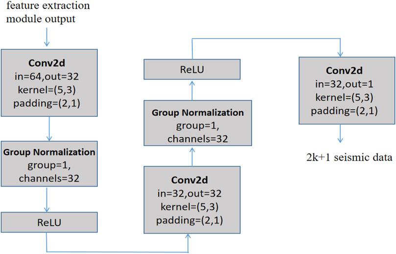
FIGURE 4. Block diagram of the forward module.

Calculate the mean square error between the feature extraction module’s input and the forward module’s output. To put it another way, the mean square error between the 2 k + 1 seismic data in the well-side trace and nearby traces and the predicted 2 k + 1 seismic data is calculated in order to update the learnable parameters in the feature extraction module and the forward module. The following Eq. 2 illustrates this:

$\begin{array}{l}{\mathit{l}}_{\mathbf{2}}=\mathit{M}\mathit{S}\mathit{E}\left({\mathit{x}}_{\mathit{i},\mathit{t}},{\widehat{\mathit{x}}}_{\mathit{i},\mathit{t}}\right)\end{array}(2)$

where ${\mathit{x}}_{\mathit{i},\mathit{t}}$ is the seismic data of the well-side and nearby 2 k traces, and ${\widehat{\mathit{x}}}_{\mathit{i},\mathit{t}}$ is the predicted 2 k + 1 seismic data.

2.3 Loss function

The loss of the entire inversion network is the mean square error between the predicted acoustic impedance data and the actual acoustic impedance ($l_1$), and the mean square error between the 2 k seismic data in and around the well-side traces and the predicted 2 k + 1 seismic data ($l_2$), with the total loss shown in Eq. 3:

$\begin{array}{l}\mathit{l}=\mathit{\alpha }{\mathit{l}}_{\mathbf{1}}+\mathit{\beta }{\mathit{l}}_{\mathbf{2}}\end{array}(3)$

where $\alpha$ and $\beta$ are weighting factors that control the effects of acoustic impedance losses and seismic losses, respectively.

2.4 Evaluation of inversion results

The inversion results are evaluated quantitatively by calculating the mean square error (MSE) and the coefficient of determination (R²) of the actual and predicted acoustic impedance.

Mean Squared Error (MSE): MSE is the average of the squared sum of the errors of the corresponding points of the predicted data and the real data, and the smaller the value indicates that the predicted data fits better with the original data, which is defined as:

$\begin{array}{l}\mathit{M}\mathit{S}\mathit{E}=\frac{\mathbf{1}}{\mathit{N}}{\displaystyle \sum }_{\mathit{i}=\mathbf{1}}^{\mathit{N}}‖{\mathit{y}}_{\mathit{i}}-{{\widehat{\mathit{y}}}_{\mathit{i}}‖}_{\mathbf{2}}^{\mathbf{2}}\end{array}(4)$

where $y_i$, ${\widehat{y}}_i$ denote the actual acoustic impedance and predicted impedance, respectively, and N is the number of data.

Determination Coefficient (R²): R² is a measure of the goodness of fit between variables that takes into account the mean square error between predicted and actual data. Its range of values is [0, 1], and the larger the value, the better the fit between the variables, the more the independent variable explains the dependent variable, and the more the independent variable contributes to the overall variation. It is defined as:

$\begin{array}{l}{\mathit{R}}^{\mathbf{2}}\left(\mathit{y},\widehat{\mathit{y}}\right)=\mathbf{1}-\frac{{\sum }_{\mathit{i}=\mathbf{1}}^{\mathit{N}}{\left({\mathit{y}}_{\mathit{i}}-{\widehat{\mathit{y}}}_{\mathit{i}}\right)}^{\mathbf{2}}}{{\sum }_{\mathit{i}=\mathbf{1}}^{\mathit{N}}{\left({\mathit{y}}_{\mathit{i}}-{\mathit{\mu }}_{\mathit{y}}\right)}^{\mathbf{2}}}\end{array}(5)$

where $y_i$, ${\widehat{y}}_i$, and ${\mu }_y$ represent the actual acoustic impedance, predicted acoustic impedance, and the average of the actual acoustic impedance, respectively. When R² is closer to 1, the stronger the correlation between the predicted and actual acoustic impedance is.

3 Experiments

The Marmousi2 and the SEAM models are widely used to validate the performance of deep learning inversion methods. This subsection will use these two models to validate the performance of the inversion network architecture proposed in this paper for acoustic impedance inversion.

3.1 Marmousi2 model inversion experiments

The Marmousi2 model is an extension of the original Marmousi model for amplitude variation with offset (AVO) analysis (Martin et al., 2002). The original Marmousi model has been widely used to validate inversion and imaging algorithms. The researchers added more complex structures representing hydrocarbon regions to the model and increased the number of strata, resulting in a new model, the Marmousi2 model, which has a width of 17 km and a depth of 3.5 km. The model is accompanied by synthetic seismic data, which are obtained by convolutional forward simulations of the model’s reflection coefficients using seismic wavelets.

The acoustic impedance model was obtained by multiplying the density and p-velocity models of the Marmousi2 data. The seismic data and acoustic impedance profiles are shown in Figures 5A, B, with 2,721 traces and 688 sampling points per trace in the seismic profile and 2,721 traces and 688 sampling points per trace in the acoustic impedance profile. The colors in Figure 5A represent seismic amplitude values, and the colors in Figure 5B represent the acoustic impedance values. Twenty traces of acoustic impedance are uniformly extracted as pseudo-well data, and for each pseudo-logging curve, 2 k + 1 seismic traces centered on the well-side trace and with k as the radius will be obtained. This paper sets k to 3, and each pseudo-logging curve corresponds to 7 seismic traces with a depth of 688 sampling points. The inverse network is trained using seismic data and pseudo-well data, the training epoch is set to 700, and the batch size is 20 for each iteration. In each training iteration, the weight coefficients in the loss function $\alpha$ and $\beta$ are set to 1. The total training loss of the previously described inverse network is calculated and back-propagated through the network.

FIGURE 5

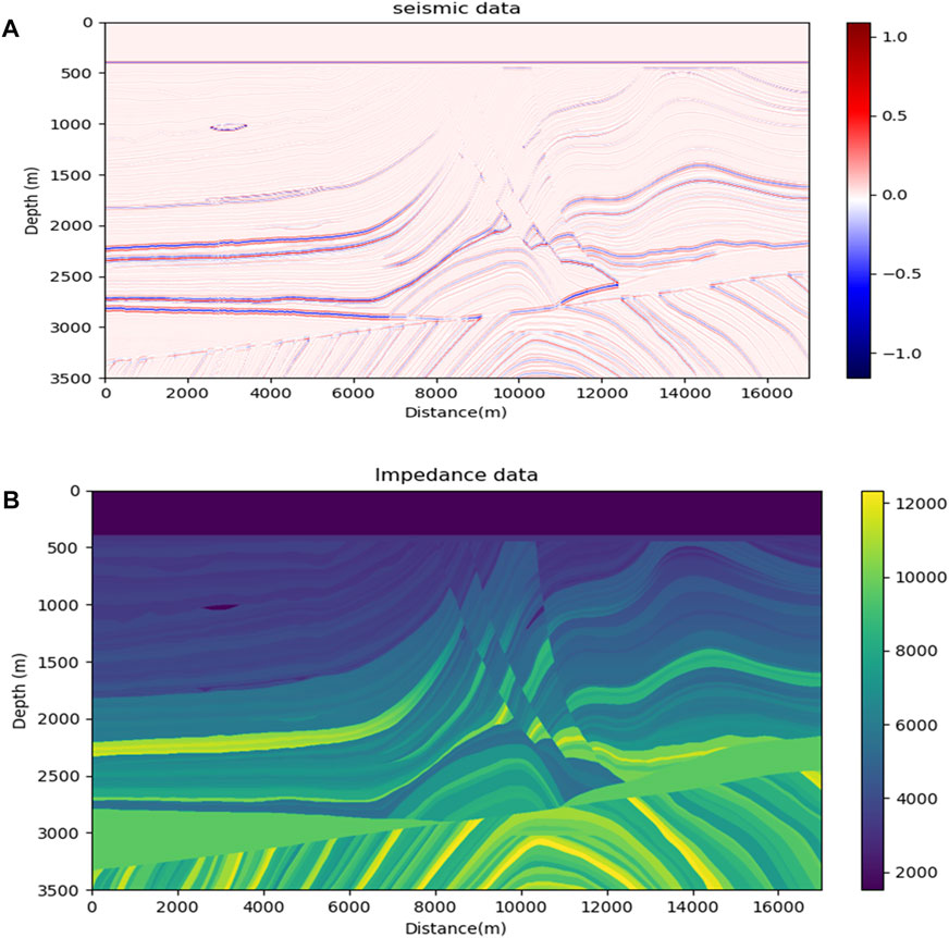
FIGURE 5. The Marmousi2 model. (A) Seismic data profile; (B) real acoustic impedance profile.

The Marmousi2 model has a complex stratigraphic structure and contains many different subsurface layered media models. The mean square error function is chosen as the loss function to measure the mean square error of the predicted and real acoustic impedance. ADAM is chosen as the optimizer, and ADAM adaptively sets the learning rate during training, with the initial learning rate set to 0.001. A weight decay of 0.0001 is chosen to limit the L₂ norm of the weights from becoming too large, reducing the risk of overfitting the network. The network’s training is implemented in the PyTorch framework, and GPUs are applied to accelerate the computation. Finally, the trained inverse network is used for acoustic impedance inversion.

In order to prove the effectiveness of this paper’s method, the inversion results of this paper’s inversion method are compared with the inversion results of the commonly used deep learning inversion methods, including the inversion method based on CNN (Das et al., 2019), the inversion method based on 1D TCN (Mustafa et al., 2019), and the inversion method based on 1D U-Net. This 1D U-net model is constructed into the same network structure as the U-net proposed in this paper, but it lacks an attention mechanism. These inverse networks are set up with the same training conditions, training data, and hyperparameters. The inversion result of the method based on CNN is shown in Figure 6A, the inversion result of the method based on 1D TCN is shown in Figure 6C, the inversion result of the method based on 1D U-Net is shown in Figure 6E, and the inversion result of the method proposed in this paper is shown in Figure 6G. Figures 6B, D, F, H correspond to the residual difference between each network’s inverse acoustic impedance and the real acoustic impedance.

FIGURE 6

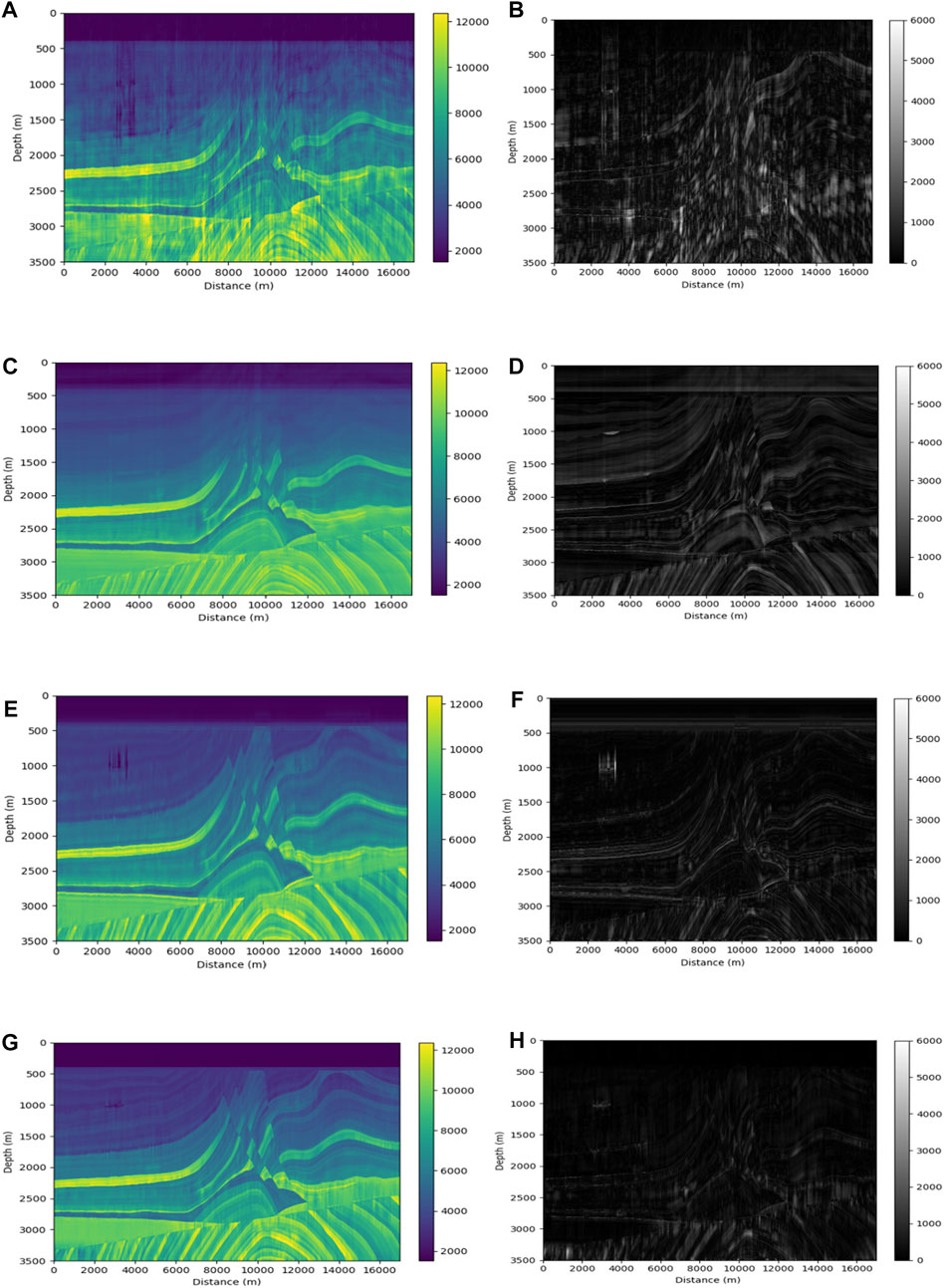
FIGURE 6. Acoustic impedance inversion profiles and residual profiles on the Marmousi2 model. (A) Inversion result of CNN method and its residual (B). (C) Inversion result of TCN method and its residual (D). (E) Inversion result of U-Net method and its residual (F). (G) Inversion result of the method in this paper and its residual (H).

As shown in Figure 6, the inversion results shown in Figures 6E, G have a higher similarity to the real model than the inversion results in Figures 6A, C. Moreover, Figure 6G has stronger horizontal continuity and weaker visible jitter in both horizontal and vertical directions for the inverse acoustic impedance profile than Figure 6E, the water layer at the top of the figure also clearly shows a relatively better inversion of Figure 6G. The partition interface and fault location in different strata are the main locations where the inversion results show errors, according to the residual profiles. In comparison to other figures in Figure 6, the inversion method in this paper can also invert the convolution structure in the model well, and the inversion results are more continuous and closer to the actual acoustic impedance, as well as more accurate in predicting the location of the faults. In most locations, the error is lower than that of other inversion methods. This is due to the effective use of the inversion network proposed in this paper for the spatial correlation of seismic data’s horizontal direction.

In order to compare the details of the inversion results of different methods from the microscopic level, the representative Trace No. 570 (corresponding to the position around x = 3,565 m) and Trace No. 1400 (corresponding to the position around x = 8,747 m) are selected for inversion.

At these two locations, the acoustic impedance values obtained by four inversion methods were compared. Figures 7A–D shows the inversion results of Trace No. 570 using the conventional CNN inversion method, the 1D TCN inversion method, the 1D U-Net inversion method, and the method proposed in this paper, with the red and black lines representing the true impedance and acoustic impedance inversion results, respectively. Similar to the inversion results of the four networks mentioned above for all seismic traces, the inversion result of the method in this paper is relatively better. The inversion result in Figure 7A has a large inversion error at a large depth, the inversion result in Figure 7B is very different from the true value, and the inversion result in Figure 7C changes too drastically, whereas the difference between the inversion result and the actual acoustic impedance in Figure 7D is very small, with the two curves almost overlapping.

FIGURE 7

FIGURE 7. Acoustic impedance inversion results of trace no. 570. (A) Inversion result of the CNN method. (B) Inversion result of the TCN method. (C) Inversion result of the 1D U-Net method. (D) Inversion result of the method in this paper.

Figures 8A–D corresponds to the inversion results of the above four methods for Trace No. 1400 seismic trace, respectively, and the conclusions are consistent with Figure 7. The inversion results of Figures 8A, B in the figure deviate more from the true values. The inversion results of Figures 8C, D are in better agreement with the actual curves, but between sampling points 0 and 100, the inversion of Figure 8D is better, while the curve change of the inversion result of Figure 8C is too drastic. This further validates the performance of the inversion network proposed in this paper.

FIGURE 8

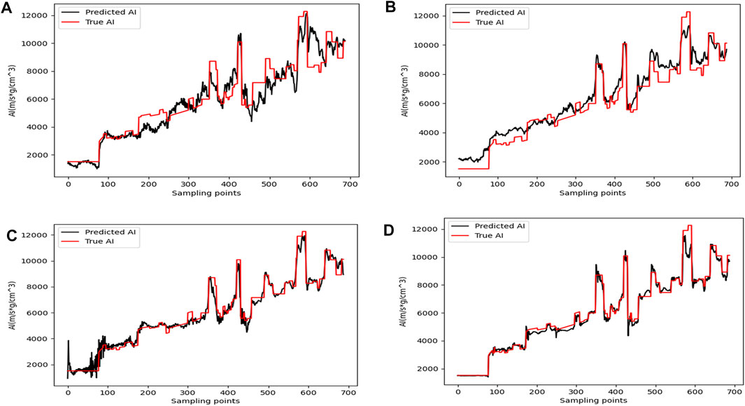
FIGURE 8. Acoustic impedance inversion results of trace no. 1400. (A) Inversion result of the CNN method. (B) Inversion result of the TCN method. (C) Inversion result of the 1D U-Net method. (D) Inversion result of the method in this paper.

In order to objectively and quantitatively evaluate the reliability of the inversion results of the four methods, the coefficients R² and MSE are used as evaluation criteria. Table 1 shows the MSE and R² between the acoustic impedance inversion results of different methods in Figure 6 and the actual acoustic impedance.

TABLE 1

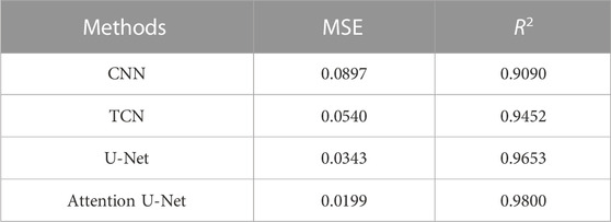
TABLE 1. MSE, R² between inversion results and actual acoustic impedance.

Table 1 shows that this paper employs multichannel inversion, and the method of acoustic impedance inversion by Attention U-Net using spatial correlation performs best in terms of MSE and R², demonstrating the method’s efficacy.

Gaussian noise of 4%, 8%, and 12% was added to the seismic data to test the adaptability of the method proposed in this paper to noise. Table 2 shows the quantitative evaluation of the inversion results obtained from the different inversion networks in Figure 6 under different noise conditions. As shown in Table 2, the performance of each method’s inversion results decreases as noise increases relative to a noiseless environment, but the performance index of the method proposed in this paper decreases the least. For example, when the noise of the seismic data increases from 4% to 12%, the R² coefficients of the inversion results of CNN, TCN, U-Net, and the proposed method decreased by 7.43%, 2.85%, 4.83%, and 1.38%, respectively. Observing the changes in MSE data leads to a similar conclusion. It can be seen that the proposed method in this paper has better noise immunity performance compared with other methods.

TABLE 2

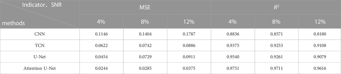
TABLE 2. MSE, R² between inversion results and actual acoustic impedance under different noise conditions.

3.2 SEAM model inversion experiments

To further verify the feasibility of the method, this paper conducts experiments with the SEAM model. The SEAM model is open source and also widely used for the validation of deep learning inversion methods (Mustafa et al., 2021). The SEAM model is a 3D seismic survey with very drastic lateral variations in density and longitudinal wave velocity, which is challenging for the inversion algorithm. The SEAM model is constructed based on basic rock properties, such as the volume of shale and sand. It follows the changing trend of shale porosity characteristics in the Gulf of Mexico, which is a better simulation of the actual geological conditions. The density of the SEAM model and the longitudinal wave velocity model are multiplied to obtain the real acoustic impedance model. The seismic data and the real acoustic impedance profiles are shown in Figures 9A, B, respectively, with 501 traces and 688 sampling points per trace in the seismic profile and 501 traces and 688 sampling points per trace in the acoustic impedance profile. 12 traces of acoustic impedance are uniformly extracted from the acoustic impedance model as pseudo-well data, and k is also set to 3, so that each pseudo-logging curve corresponds to 7 seismic traces with a depth of 688 sampling points. The training epoch is set to 400, and the batch size is 12 for each iteration. The network is then trained in the same way as the Marmousi2 model, and the trained network is used to perform acoustic impedance inversion on all seismic traces.

FIGURE 9

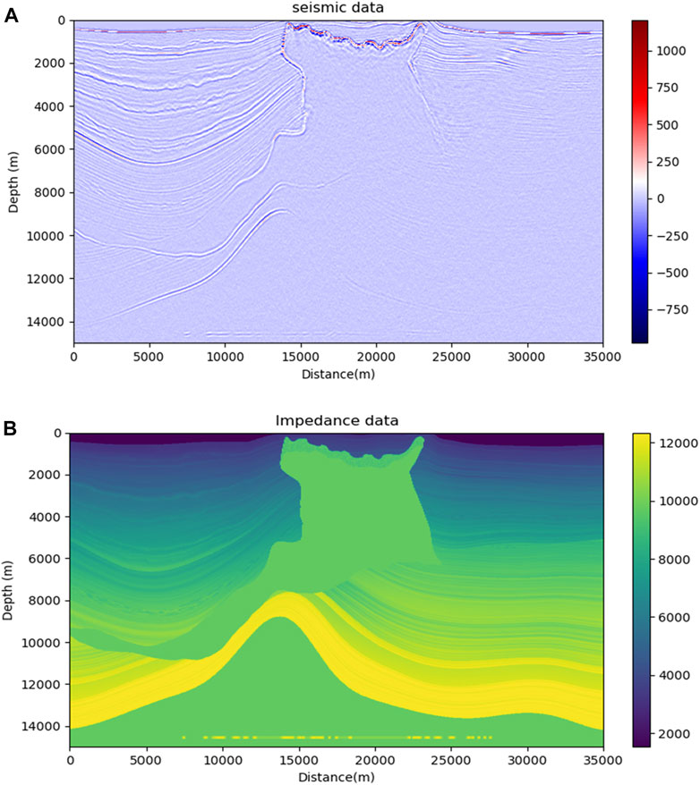
FIGURE 9. SEAM model. (A) Seismic data profile. (B) Real acoustic impedance profile.

The inversion results are shown in Figure 10. Figures 10A, C, E correspond to the results of the inversion based on the conventional CNN inversion method, the 1D U-Net inversion method, and the inversion of the proposed method in this paper, respectively. Figures 10B, D, F correspond to the residuals between the acoustic impedance and the real acoustic impedance inverted by each method, respectively. As can be seen from the figure, compared with Figures 10C, E has a better effect in displaying the stratigraphic interface in the left half of the depth range of 10,000 m to 14,000 m, and the strata are clearer. Some thin stratigraphic variations can be clearly observed in the upper left part of Figure 10E diagram between 5,000 and 9,000 m depth. For example, at 2,500 m depth in the real model, there is a thin arc-shaped stratigraphy that can be seen more clearly in Figure 10E, whereas it is difficult to see in Figures 10A, C, and Figure 10A does not outline the central uplifted area in the real model better. Although the method in this paper has some errors in the inversion of the SEAM model, the overall effect is better than the other two methods.

FIGURE 10

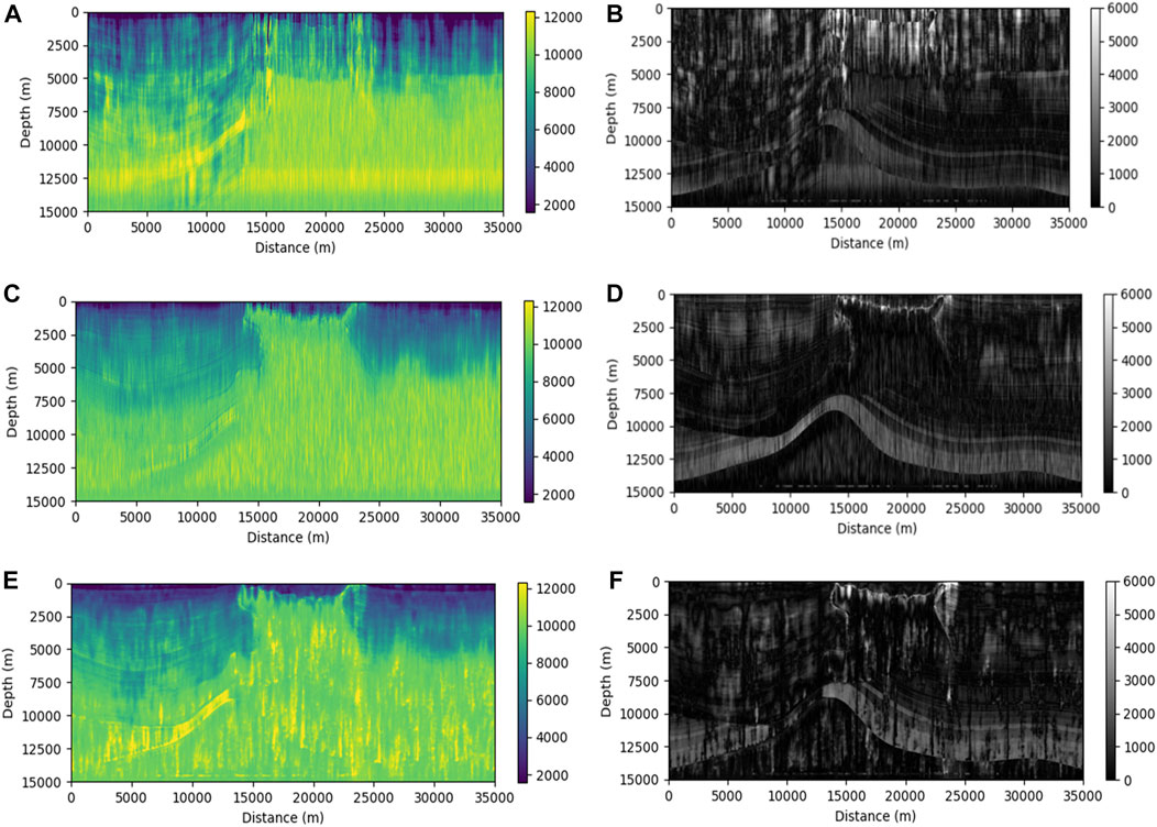
FIGURE 10. Acoustic impedance inversion profiles and residual profiles on the SEAM model. (A) Inversion result of CNN method and its residual (B). (C) Inversion result of U-Net method and its residual (D). (E) Inversion result of the method in this paper and its residual (F).

Trace No. 179 (corresponding to the vicinity of x = 12,500 m) was selected for the inversion experiment, and the acoustic impedance inversion results of the three inversion methods are shown in Figure 11. Figures 11A–C shows the inversion results of Trace No. 179 using the conventional CNN inversion method, the 1D U-Net inversion method, and the method proposed in this paper, with the red and black lines representing the true impedance and acoustic impedance inversion results, respectively. The proposed method has better inversion results compared with other methods. From Figure 11C, we can see that the inversion result obtained by the proposed method almost completely overlaps with the true impedance, while the inversion result of the CNN deviates from the true value, and the result obtained by the 1D U-Net inversion method also has large deviations, with a large deviation at a small depth.

FIGURE 11

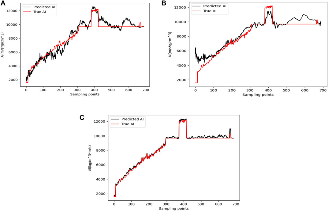
FIGURE 11. Acoustic impedance inversion results of trace no. 179. (A) Inversion result of the CNN method. (B) Inversion result of the 1D U-net method. (C) Inversion result of the method in this paper.

To quantitatively evaluate the performance of the method proposed in this paper, the MSE and the R² between the acoustic impedance inversion results and the true acoustic impedance are calculated and presented in Table 3. The data are the MSE and R² between the acoustic impedance and the true acoustic impedance obtained by the inversion of different inversion methods in Figure 10. The data in the table show that the inversion result of the proposed method performs best in terms of MSE and R², which verifies the effectiveness of the method.

TABLE 3

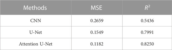
TABLE 3. MSE, R² between inversion results and actual acoustic impedance.

4 Conclusion

This paper proposes a multichannel seismic acoustic impedance inversion method based on the Attention U-Net network. Different from the conventional supervised learning inversion method, this inversion method applies the spatial correlation in the horizontal direction to the inversion network, and trains the network with 2 k + 1 seismic traces centered on the well-side trace and the corresponding logging curve to enhance the lateral continuity. In addition, the Attention U-Net network is used as a feature extraction module in the inversion network, and the attention gating model is added to the traditional U-Net-based inversion network. The AG is used to implicitly learn to suppress irrelevant regions in the input data while emphasizing salient features useful for inversion results, and it can be easily integrated into the standard CNN architecture to reduce computational overhead while improving the model’s sensitivity and prediction accuracy. The method’s performance is evaluated using the Marmousi2 and SEAM models, and it is also compared to several other commonly used deep learning inversion methods. The results show that the inversion results of the method proposed in this paper are more consistent with the actual acoustic impedance values, and the anti-noise performance is the best. In the SEAM model, where the lateral velocity and density vary drastically, the proposed method can better obtain the stratigraphic structure and details in the true model. These are attributed to the combined application of the attention gating model and methods such as multichannel simultaneous inversion.

Data availability statement

Publicly available datasets were analyzed in this study. This data can be found here: https://github.com/amustafa9/Geophysics-2021-Joint-learning-for-spatial-context-based-inversion/blob/master/data.zip.

Author contributions

JN responses for the experiments of the work and drafting papers. SL responses for the concept and design of the work and revisions to the paper. ZW and XY responses for important revisions to the papers.

Funding

This research was funded by the National Natural Science Foundation of China (Nos. 42164006 and 62161012), the Hunan Provincial Natural Science Foundation of China (No. 2022JJ30474), the China Postdoctoral Science Foundation (No. 2021M700682) and the Scientific Research Fund of Hunan Provincial Education Department (No. 21B0507).

Conflict of interest

The authors declare that the research was conducted in the absence of any commercial or financial relationships that could be construed as a potential conflict of interest.

Publisher’s note

All claims expressed in this article are solely those of the authors and do not necessarily represent those of their affiliated organizations, or those of the publisher, the editors and the reviewers. Any product that may be evaluated in this article, or claim that may be made by its manufacturer, is not guaranteed or endorsed by the publisher.

References

Aleardi, M., and Salusti, A. (2021). Elastic prestack seismic inversion through discrete cosine transform reparameterization and convolutional neural networks. Geophysics 86 (1), R129–R146. doi:10.1190/geo2020-0313.1

CrossRef Full Text | Google Scholar

Alfarraj, M., and AlRegib, G. (2018). “Petrophysical property estimation from seismic data using recurrent neural networks,” in SEG technical program expanded abstracts 2018 (United States: Society of Exploration Geophysicists). .

CrossRef Full Text | Google Scholar

Cao, D., Su, Y., and Cui, R. (2022). Multi-parameter pre-stack seismic inversion based on deep learning with sparse reflection coefficient constraints. J. Petroleum Sci. Eng. 209, 109836. doi:10.1016/j.petrol.2021.109836

CrossRef Full Text | Google Scholar

Chen, L.-C., Papandreou, G., Kokkinos, I., Murphy, K., and Yuille, A. L. (2017). Deeplab: Semantic image segmentation with deep convolutional nets, atrous convolution, and fully connected crfs. IEEE Trans. pattern analysis Mach. Intell. 40 (4), 834–848. doi:10.1109/tpami.2017.2699184

PubMed Abstract | CrossRef Full Text | Google Scholar

Cho, K., Van Merriënboer, B., Gulcehre, C., Bahdanau, D., Bougares, F., Schwenk, H., et al. (2014). “Learning phrase representations using RNN encoder-decoder for statistical machine translation,”. arXiv preprint arXiv:1406.1078.

CrossRef Full Text | Google Scholar

Das, V., Pollack, A., Wollner, U., and Mukerji, T. (2019). Convolutional neural network for seismic impedance inversion. Geophysics 84 (6), R869–R880. doi:10.1190/geo2018-0838.1

CrossRef Full Text | Google Scholar

Du, J., Liu, J., Zhang, G., Han, L., and Li, N. (2019). “Pre-stack seismic inversion using SeisInv-ResNet,” in SEG technical program expanded abstracts 2019 (United States: Society of Exploration Geophysicists).

CrossRef Full Text | Google Scholar

Graves, A., Mohamed, A.-r., and Hinton, G. (2013). “Speech recognition with deep recurrent neural networks,” in IEEE international conference on acoustics, speech and signal processing, Singapore, 22-27 May 2022.

CrossRef Full Text | Google Scholar

Ioffe, S., and Szegedy, C. (2022). “Batch normalization: Accelerating deep network training by reducing internal covariate shift,” in International conference on machine learning: PMLR, USA, 25-27 July 2022, 448–456.

Google Scholar

Krizhevsky, A., Sutskever, I., and Hinton, G. E. (2017). Imagenet classification with deep convolutional neural networks. Commun. ACM 60 (6), 84–90. doi:10.1145/3065386

CrossRef Full Text | Google Scholar

Martin, G. S., Larsen, S., and Marfurt, K. (2002). Marmousi-2: An updated model for the investigation of AVO in structurally complex areas. Salt Lake City: SEG Annual Meeting: OnePetro.

Google Scholar

Mustafa, A., Alfarraj, M., and AlRegib, G. (2019). “Estimation of acoustic impedance from seismic data using temporal convolutional network,” in SEG technical program expanded abstracts 2019 (United States: Society of Exploration Geophysicists). .

CrossRef Full Text | Google Scholar

Mustafa, A., Alfarraj, M., and AlRegib, G. (2021). Joint learning for spatial context-based seismic inversion of multiple data sets for improved generalizability and robustness. Geophysics 86 (4), O37–O48. doi:10.1190/geo2020-0432.1

CrossRef Full Text | Google Scholar

Nair, V., and Hinton, G. E. (2010). “Rectified linear units improve restricted Boltzmann machines,” in Proceedings of the 27th International Conference on Machine Learning, Haifa, Israel, June 21-24, 2010.

Google Scholar

Oktay, O., Schlemper, J., Folgoc, L. L., Lee, M., Heinrich, M., Misawa, K., et al. (2018). “Attention u-net: Learning where to look for the pancreas,”. arXiv preprint arXiv:1804.03999.

Google Scholar

Ren, S., He, K., Girshick, R., and Sun, J. (2015). Faster r-cnn: Towards real-time object detection with region proposal networks. Adv. neural Inf. Process. Syst. 28, 1. doi:10.1109/TPAMI.2016.2577031

CrossRef Full Text | Google Scholar

Ronneberger, O., Fischer, P., and Brox, T. (2015). “U-net: Convolutional networks for biomedical image segmentation,” in International Conference on Medical image computing and computer-assisted intervention, Germany, October 8-12, 2023.

CrossRef Full Text | Google Scholar

Treitel, S., and Lines, L. (2001). Past, present, and future of geophysical inversion—a new millennium analysis. Geophysics 66 (1), 21–24. doi:10.1190/1.1444898

CrossRef Full Text | Google Scholar

Vinyals, O., Toshev, A., Bengio, S., and Erhan, D. (2022). “"Show and tell: A neural image caption generator,” in Proceedings of the IEEE conference on computer vision and pattern recognition, San Juan, PR, USA, 17-19 June 1997.

Google Scholar

Wang, Y., Ge, Q., Lu, W., and Yan, X. (2020). Well-logging constrained seismic inversion based on closed-loop convolutional neural network. IEEE Trans. Geoscience Remote Sens. 58 (8), 5564–5574. doi:10.1109/tgrs.2020.2967344

CrossRef Full Text | Google Scholar

Wu, B., Meng, D., Wang, L., Liu, N., and Wang, Y. (2020). Seismic impedance inversion using fully convolutional residual network and transfer learning. IEEE Geoscience Remote Sens. Lett. 17 (12), 2140–2144. doi:10.1109/lgrs.2019.2963106

CrossRef Full Text | Google Scholar

Wu, X., Yan, S., Bi, Z., Zhang, S., and Si, H. (2021). Deep learning for multidimensional seismi impedance inversion. Geophysics 86 (5), R735–R745. doi:10.1190/geo2020-0564.1

CrossRef Full Text | Google Scholar

Wu, Y., and He, K. (2012). “Group normalization,” in Proceedings of the European conference on computer vision (ECCV)), Florence Italy, October 7 - 13, 3–19.,

Google Scholar