 Ming Zhao
 Zhuowei Xiao
 Miao Zhang
 Yun Yang
 Lin Tang6
 Shi Chen
- 1Institute of Geophysics, China Earthquake Administration, Beijing, China
- 2Beijing Baijiatuan Earth Sciences National Observation and Research Station, Beijing, China
- 3Department of Earth and Environmental Sciences, Dalhousie University, Halifax, NS, Canada
- 4Institute of Geology and Geophysics, Chinese Academy of Sciences, Beijing, China
- 5Earthquake Monitoring Centre, Jiangsu Earthquake Administration, Nanjing, China
- 6Earthquake Monitoring Centre, Sichuan Earthquake Administration, Chengdu, China
Accurate P-wave first-motion-polarity (FMP) information can contribute to solving earthquake focal mechanisms, especially for small earthquakes, to which waveform-based methods are generally inapplicable due to the computationally expensive high-frequency waveform simulations and inaccurate velocity models. In this paper, we propose a deep-learning-based method for the automatic determination of the FMPs, named “DiTingMotion”. DiTingMotion was trained with the P-wave FMP labels from the “DiTing” and SCSN-FMP datasets, and it achieved ∼97.8% accuracy on both datasets. The model maintains ∼83% accuracy on data labeled as “Emergent”, of which the FMP labels are challenging to identify for seismic analysts. Integrated with HASH, we developed a workflow for automated focal mechanism inversion using the FMPs identified by DiTingMotion and applied it to the 2019 M 6.4 Ridgecrest earthquake sequence for performance evaluation. In this case, DiTingMotion yields comparable focal mechanism results to that using manually determined FMPs by SCSN on the same data. The results proved that the DiTingMotion has a good generalization ability and broad application prospect in rapid earthquake focal mechanism inversion.
Introduction
In recent years, the rapid development of dense arrays and real-time seismology technology has brought seismology into a new era. For example, there are over 5,000 broadband and over 10,000 strong motion seismic stations in China, and all data are transmitted to the data center in real time via the Internet. The extensive volume of data brings great challenges to routine earthquake cataloging and rapid focal mechanism determination. The focal mechanisms can be solved from the P-wave first-motion-polarity (FMP) information (e.g., HASH; Hardebeck & Shearer, 2002; Hardebeck & Shearer, 2003) or the waveform information (e.g., gCAP; Zhao & Helmberger, 1994; Zhu & Helmberger, 1996; Zhu & Zhou, 2016). However, the waveform-based methods suffer the high-computational cost of high-frequency seismogram simulations and inaccurate velocity models when applied to small earthquakes (e.g., M < 3) and generally require manual interventions. The polarity-based methods rely on accurate FMP information that used to be determined manually. In this study, we focus on the automatic determination of FMPs and their application to earthquake focal mechanism inversion.
P-wave FMP determination methods have been developed mainly based on waveform amplitude change before and after the arrivals (e.g., Chen & Holland, 2016; Pugh et al., 2016). However, their accuracy is less than that of human experts, especially for low signal-to-noise ratio phases and slow-starting phases. In recent years, machine learning has been widely used in all aspects of automated seismic data processing, including seismic data denoising (Zhu W et al., 2019), earthquake detection (Perol et al., 2018; Saad et al., 2020; Saad et al., 2022a), seismic phase picking (Ross et al., 2018a; Wang et al., 2019; Zhou et al., 2019; Mousavi et al., 2020; Saad et al., 2021; Xiao et al., 2021), phase association (Ross et al., 2019b), earthquake location (e.g., van den Ende et al., 2020; Zhang et al., 2022), magnitude estimation (Mousavi & Beroza, 2020; Saad et al., 2022b), and earthquake early warning (Zhang et al., 2021). It has also been used in the FMP identification (e.g., Ross et al., 2018b; Uchide et al., 2020; Cheng et al., 2021), which considers FMP identification as a typical classification problem and uses the convolutional neural network (CNN) model with the classical structure for the automatic prediction of the “up” or “down” FMPs of P phases.
In this paper, we propose a deep CNN model to identify P-wave FMPs, the so-called “DiTingMotion”. Compared to previous studies that determine FMP with deep learning, this study has distinct features as follows: i) In terms of data, we extend the training set by combining both the DiTing (Zhao et al., 2022) and SCSN-FMP (Ross et al., 2018b) datasets; ii) In terms of deep-learning model, we designed a novel formulation of the input, proposed a CNN with side-output layers for FMP classification, and used the focal loss instead of classic cross-entropy for training; iii) In terms of evaluation, we demonstrate that DiTingMotion provides high accuracy and generalization ability in different test datasets as well as real-world applications. We build a workflow to automatically obtain focal mechanisms from continuous seismic waveforms and apply it to the 2019 Ridgecrest earthquake sequence for performance evaluation. We compare our automatic focal mechanism result with the SCSN routine focal mechanism catalog. The results show that with accurate P arrival time picking, the DiTingMotion can reliably identify P-wave FMPs with comparable accuracy as manual FMPs. Furthermore, it can complement events with insufficient manual FMPs to improve the focal mechanism solution.
Methodology
Design of the neural network
Figure 1 shows the network architecture of the “DiTingMotion” neural network. It has five convolutional blocks, the first two consist of two 1D convolutions and one max-pooling layer. The last three blocks contain three 1D convolutions and one max-pooling layer, and a side layer follows the last convolutional layer of each block. These five side layers aggregate to form the final output and output the classification probability with a sigmoid activation function. The “Up” and “Down” polarity is then determined by comparing the classification probability with the threshold. The network architecture is developed from holistically-nested edge detection (HED) (Xie & Tu, 2015). One advantage of the HED is that it has side outputs attached to CNN layers. The CNN layer gets a larger receptive field as the network proceeds deeper. Thus, the final output can capture patterns at different levels and scales by combining all the side outputs. Besides, HED uses deep supervision in training, which enables the shallow layers to be trained more adequately. The HED is originally designed to detect fine features of object edges. The targets of interest in P-wave FMP determination are the edge features around the P wave arrival. For the details of the model, e.g., CNN kernel size, number of layers, and number of CNN blocks, etc., please see Supplementary Table S1 in the electronic supplement.
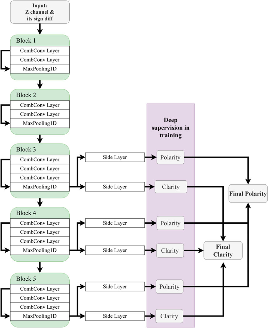
FIGURE 1. Diagram showing the DiTingMotion deep-learning neural network.
In addition to using raw vertical component slices centered at P arrivals for FMP determination, the “DiTingMotion” takes the sign function of the difference of the vertical waveform after the P wave arrival time as another input, which is calculated as follows:
where
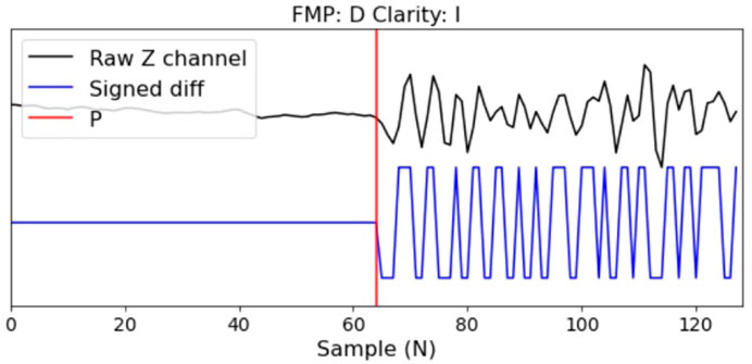
FIGURE 2. An example of the input data includes the raw vertical waveform (upper trace) and its corresponding sign function (lower trace).
The output of “DiTingMotion” includes the polarity sign and clarity. For polarity signs, there are “up” (U), “down” (D), and “uncertain” (x). For clarity signs, there are “impulsive” (I), “emergent” (E), and “uncertain” (−). Note that we only use the “x” class for polarity in training for the compatibility of the SCSN-FMP dataset. In testing, we force the network to predict between the “U” and “D”.
Training, validation and testing
We trained the DiTingMotion using both DiTing and SCSN-FMP datasets. The DiTing dataset is a large-scale Chinese seismic benchmark dataset that has 641,025 high-quality P-wave FMP labels from >1300 broadband and short-period seismometers distributed throughout China with epicenter distance up to ∼330 km from 2013 to 2020 (Zhao et al., 2022). The DiTing dataset not only contains polarity information (“U”, “D”) but also includes the corresponding clarity instructions (“I”, “E”, and “x”). The SCSN-FMP dataset contains ∼4.84 million seismograms, with epicenter distances < ∼100 km (Ross et al., 2018b). For the DiTing dataset, we randomly split 75%, 10%, and 15% of the DiTing dataset for training, validation, and testing, respectively. For the SCSN-FMP dataset, we use ∼2.49 M samples for the training process (90% for training and 10% for validation) and ∼2.35 M samples for testing.
During the training process, we use a data augmentation that flips the seismograms and their corresponding labels, which is similar to Uchide (2020). We use the Adam optimizer with a learning rate of 0.0003 (Kingma & Ba, 2014) for optimizing the loss function. Dropout (Srivastava et al., 2014) and early stopping strategies are applied to avoid the overfitting problem. We use the focal loss function (Lin et al., 2017) to train DiTingMotion. The FL is formulated as the following:
Here
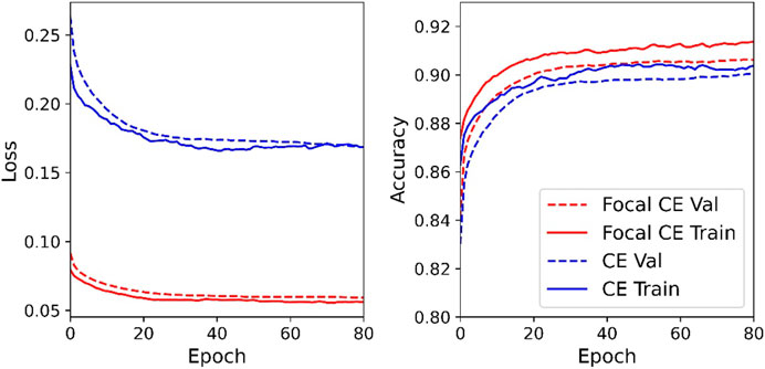
FIGURE 3. The training and validation curves for cross entropy (CE) and focal cross entropy (Focal CE).
We then test the well-trained DiTingMotion model using the DiTing and SCSN-FMP test sets. We use the confusion matrix to evaluate the model performance. As Figure 4 shows, high accuracy on both the two test sets are achieved: the model can achieve ∼97% accuracy for both “U” and “D” polarities, which proves that the DiTingMotion model has comparable performance to the model trained by Ross et al. (2018b) on the SCSN-FMP dataset (i.e., 95%) and keeps the same good performance on the DiTing dataset that recorded by the China Seismological Network. Besides, importantly, due to the specially designed sign function for the emergent FMPs, the DiTingMotion model has relatively robust performance on data with less clear FMPs. We test an independent test set (from the DiTing dataset) with 3934 “E” clarity labeled samples, the predicted accuracy drops but still achieves ∼83% (Figure 4C). The training and testing of the model are performed on an Nvidia Telsa V100s GPU card and the application time is 41.7 ms ± 880 µs per loop (mean ± std. dev. of 7 runs, 10 loops each) for predicting one sample from a single station.
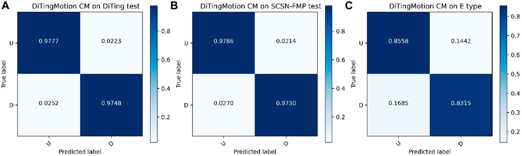
FIGURE 4. The DiTingMotion confusion matrix (CM) on the test set of DiTing (A), SCSN-FMP (B), and samples with “E” clarity from the DiTing dataset (C). The X-axis is the prediction, and the Y-axis is the true label.
Workflow for focal mechanism inversion
With reliable FMP prediction, we can further use the HASH method to invert the focal mechanism, which is a widely used polarity-based focal mechanism determination program developed by Hardebeck and Shearer (2002), Hardebeck and Shearer (2003). The main reason why HASH is suitable for our automatic workflow is that it accounts for possible errors in earthquake locations and velocity models, as well as the tolerance of a certain number of wrong FMPs. On the other hand, HASH has demonstrated excellent performance for focal mechanism inversion in other similar studies using machine learning (ML) based FMPs (e.g., Ross et al., 2018b; Uchide et al., 2020; Cheng et al., 2021).
Figure 5 shows the workflow, the code. The input of the HASH method is the source location, station locations, seismic velocity model, P-wave FMPs, and S/P amplitude ratios, then it will compute takeoff angles and perform a grid search over the strike, dip, and rake to find the set of acceptable focal mechanism solutions. If there are multiple solutions that fit all the impulsive polarities, HASH chooses the solution with the minimized number of misfit emergent FMPs. The earthquake locations and phase arrivals can be accessed from the routine phase file (e.g., via the Southern California Seismic Network—SCSN). Based on the manual picks, DiTingMotion predicts P-wave FMPs from sliced waveforms, which will be utilized by HASH for focal mechanism inversion along with S/P amplitude ratios. With the aid of recently developed ML-based phase pickers, earthquake catalogs (with locations and arrivals) also can be automatically built from continuous waveforms, for example, via the LOC-FLOW developed by Zhang et al. (2022).
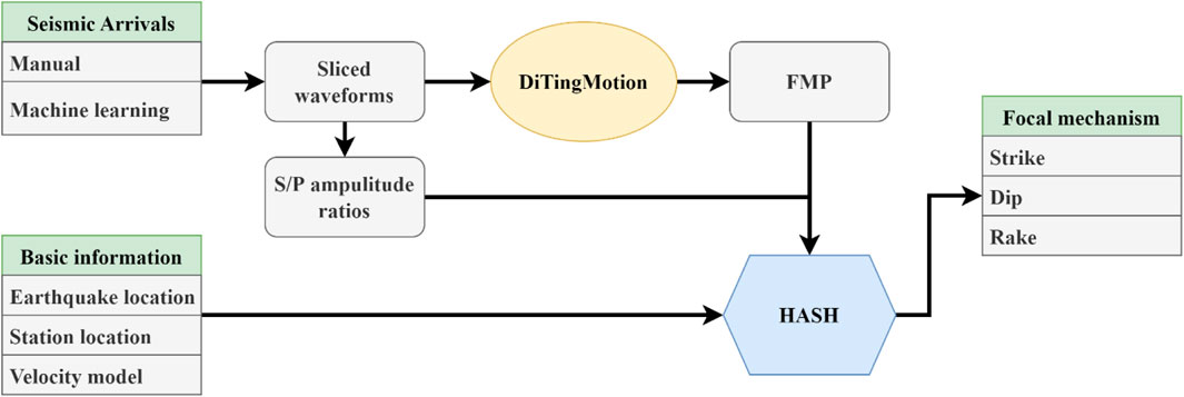
FIGURE 5. Workflow showing HASH focal mechanism inversion using DiTingMotion.
Application to the 2019 ridgecrest earthquake sequence
We use the 4 July 2019 Ridgecrest earthquake sequence in southern California as a case study to evaluate the performance of our workflow. We choose this region and this earthquake sequence because 1) the HASH method has already been routinely used by the SCSN for a long time (Yang et al., 2012), and most importantly, 2) focal mechanisms of the earthquake sequence have been well studied using the HASH method (Lin et al., 2020) and waveform-based gCAP3D method (Wang et al., 2019), which provide us with independent benchmarks.
From the first foreshock of the MW 6.4 on 17:33:48, 4 July to the aftershocks that occurred following the MW 7.1 through 23:59:59, 9 July 2019, a total of 1,241 events with magnitude
Firstly, we assessed the impact of P arrival time accuracy on FMP results. Since the quantity and quality of FMPs for each event are critical to the focal mechanism inversion, for a fair comparison, we screened out 529 common events from the SCSN catalog and ML catalog (Liu et al., 2020), with at least 15 common associated P arrival times, and magnitudes range from 2.5 to 4.9. These events have 11,980 P common arrival times and 10,347 P-wave FMPs from the SCSN catalog. First, we test the performance of DiTingMotion on the manual P arrivals from the SCSN. The accuracy of FMP identification can achieve 89.9% U) and 89% D), respectively (Figure 6A). Among the 11,980 P waveforms, there are 1,634 FMPs with clarity of “x” (uncertain), while DiTingMotion identified 1,187 of them (i.e., 546 up and 641 down), and only 447 were evaluated as “x” (Figure 6A). Although we do not have labels to evaluate the accuracy for these additional predictions, we find that these ML-discovered FMPs are a good complement to focal mechanism inversion through the later result comparisons. Second, we test the performance of DiTingMotion on the ML arrivals from Liu et al. (2020). We find a significant decrease in accuracy (i.e., 71.3%(U) and 74.6%(D); Figure 6B), suggesting that the marked P arrivals affect the FMP identification in DiTingMotion. We compare the arrival difference between the manual arrivals and ML arrivals and find that the ML arrivals may have 0 ∼ ± 0.1s difference (with a majority of differences < 0.05 s) from the manual picks (see Supplementary Figure S1 in the electronic supplement). To verify the tolerance of pick uncertainties in DiTingMotion, we perturb the P manuals arrivals by ± 0.05 s and re-evaluate its performance. Results show that the accuracy reduces to 81.8% (U) and 80.3% (D) (Figures 6C, D) and it drops more when the arrival time used is before the true time (Figure 6C). It suggests that the accuracy of arrival time picking has a significant impact on DiTingMotion for FMP identification because the sign function we use as input exactly starts from the P arrivals.
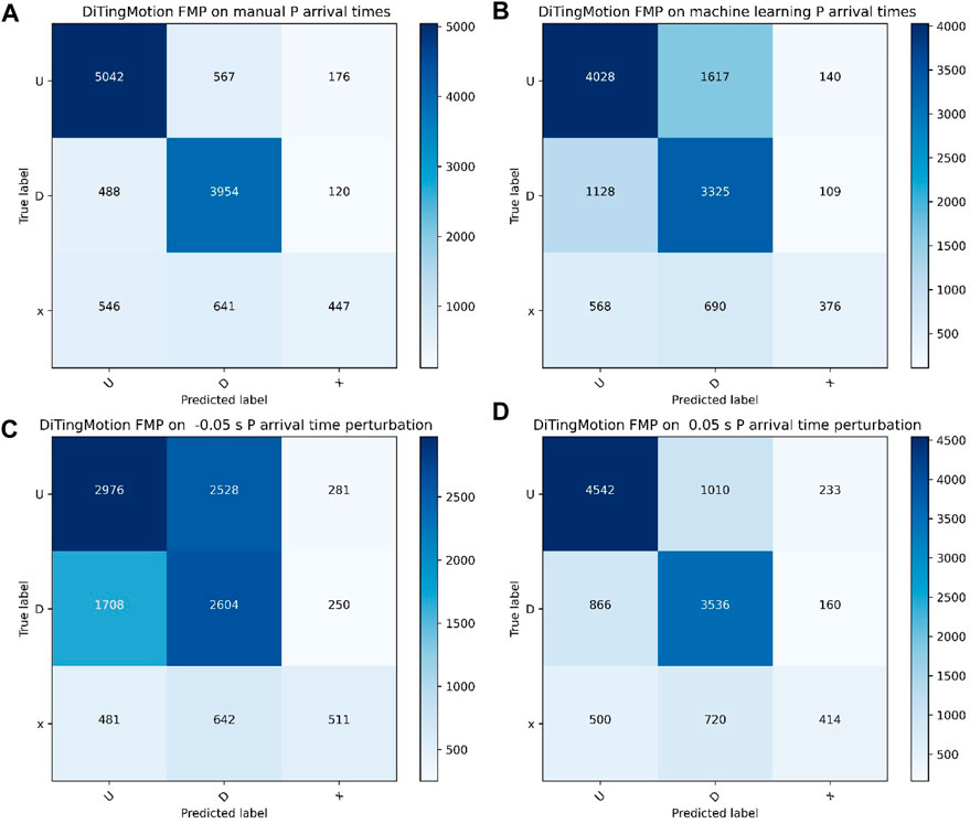
FIGURE 6. The confusion matrix of FMPs according to different P arrival times: (A) manual P picks from SCSN; (B) machine learning P picks from Liu et al., 2020; (C) 0.05s earlier than the manual P arrivals; (D) 0.05s later than the manual P arrivals.
Secondly, we compared three HASH focal mechanisms obtained using different FMP inputs. Common events between the SCSN focal mechanism catalog, Lin et al. (2020)’s and Wang and Zhan (2020)’s are selected for result comparison. The first two focal mechanism catalogs are done by HASH, while the latter is obtained through waveform inversion. For HASH results, we only choose focal mechanisms with quality “A” and “B” from the SCSN catalog and Lin et al. (2020)’s since quality “C” and “D” results have large uncertainties. For waveform inversion-based focal mechanisms (Wang and Zhan, 2020), we use them all because they are verified by waveform fitting and are reliable. Based on the above selection criteria, 450 events from the SCSN catalog, 247 events from Lin’s catalog, and 116 events from Wang’s catalog are selected. There are three kinds of FMP input for focal mechanism inversions: 1. ML FMP based on manual picks (“ML” for short); 2. Manual FMP (“Man” for short); 3. Manual FMP, supplemented by ML FMP based on manual picks (“Man+ML” for short). To quantitatively characterize the difference between these results, we adopt the Kagan angle analysis (Kagan, 2007), in which the Kagan angle represents the difference in rotation angle between two independent focal mechanisms. Figure 7 shows the corresponding Kagan angles between the three inversion results and the three reference catalogs. The comparison results with the three catalogs are consistent: the Kagan angles are mainly distributed in the [10°,30°] interval in all the results, and the 80% lines are around 40°. The 80% line is to show which result is the closest to the reference catalog. “Man+ML” is the best in the comparison with SCSN catalog and Wang et al. (2019), and slightly worse than “Man” in Lin et al. (2020), which proves ML FMP can be a useful supplement to the manual FMP. It is also worth mentioning that the result difference between “Man” and “ML” is minor using the SCSN as a reference (Figure 7A), which means if the P arrival time picking is accurate, ML FMP alone can be sufficiently good for the HASH focal mechanism inversion.

FIGURE 7. The histograms of Kagan angles according to three HASH results with different inputs: manual FMP combined with machine learning FMP (blue), manual FMP only (yellow), and machine learning FMP using manual picks (green). The 80% line indicates that the number to the left of the line accounts for 80% of the total. (A) Compare with SCSN catalog; (B) Compare with Lin et al. (2020); (C) Compare with Wang and Zhan (2020); (D) Venn diagram of three HASH results with Kagan angle larger than 40°.
Most inversion results with Kagan angles distributed in the [10°, 30°] interval are reliable, like Figure 8A shows, different results have very close focal mechanism solutions and have few inconsistencies in the FMP inputs. Since ML usually identifies more FMPs, in some cases the ML provides the best solution, for example, in Figure 8B, there are 8 “x” in the manual FMP while only 1 in ML FMP, due to the FMP number is not enough, the Man result doesn’t constrain well, and even Man+ML is not as good as ML, that means there is obvious wrong FMP in Man results (like “WRC2”), since all the other inputs are exactly the same for all three results.
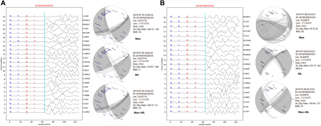
FIGURE 8. Two examples (A, B) of focal mechanism solution comparisons with different FMP inputs. (A, B, left) P waveforms with arrival times (dash-dotted green lines), ML FMP and sharpness (blue texts), and manual FMP and sharpness (red texts). (A, B, right) The corresponding focal mechanisms from the ML, Man, Man+FML FMPs, with FMP signs and station locations on the beach balls.
However, in addition to FMP inputs, many other factors would also affect the final inversion results, for example, the azimuth distribution of stations, the signal-to-noise ratio of data, the choice of velocity models, or different HASH parameters settings. All these factors make it seems quite normal to have up to 40° Kagan angle differences between different results (a comparison between the three reference catalogs we used in this paper is available in Supplementary Figure S2). We thus performed an analysis of events with Kagan angle large than 40°, as the Venn diagram in Figure 7D shows, there are 52 events simultaneously present in all the results. After checking their P waves with ML and manual FMPs, we found that most of these events were related to seven stations: “JRC2” (49 related), “WVP2” (48 related), “WHF” (46 related), “MPM” (46 related), “CLC” (45 related), “WRC2” (38 related), “WCS2” (32 related). By calculating the confusion matrix of these stations separately (see Supplementary Figure S3 in the electronic supplement), we found that the ML FMP identification accuracy of these stations (81%–88%) is indeed relatively lower than the overall level (89.9%). The discrepancies between different results may be because individual waveforms have low signal-to-noise ratios, resulting in controversial FMPs (see an example in Supplementary Figure S4A). Of course, we cannot exclude that the reference solution itself is wrong (see Supplementary Figure S4B).
Discussion and conclusion
We have developed a novel machine-learning algorithm for the efficient identification of P-wave FMP from raw seismic waveforms. This method is developed from the network architecture for edge detection in image recognition, and in addition to using the original P waveform, the sign function of the difference of the vertical waveform after the P wave arrival time was also used to enhance the input features. The model trained with the above strategies resulted in strong generalization ability: 1) the model reached 97.3% (“D”) and 97.86% (“U”) accuracy on the SCSN test dataset, and 97.48%(“D”) and 97.77%(“U”) accuracy on the DiTing dataset; 2) the model achieved 85.58% (“U”) and 83.15% (“D”) for the recognition of the challenging “emergent” labeled data.
Though the use of sign functions as input enhances the ability to recognize all kinds of FMP features, on the other hand, the algorithm also becomes more sensitive to the accuracy of P arrival time. A test on 10,347 P waveforms showed that even 0.05 s disturbances in P arrival time could significantly affect FMP identification results (e.g., Figures 6C, D). This is different from the model developed by Ross et al. (2018b) and Uchide (2020), in which they augmented the data by time shift and made the model more flexible to the uncertainties in arrival-time picking. However, improving the tolerance for time shifts would decrease the polarity classification performance, especially for complex examples. In our opinion, the phase picking accuracy should be considered by picking algorithms or seismic analysts rather than a polarity determination model.
We have applied DiTingMotion to the automatic focal mechanism inversion workflow. Given the accurate P arrival times, the accuracy of FMP identification can achieve 89.9% (U) and 89% (D), respectively, when compared with manual FMP in the SCSN catalog. We evaluate three HASH solutions derived from different sources of FMPs by calculating the Kagan angle between our results and three reference focal mechanism catalogs, in which we find ML FMP can be a valuable supplement to the manual FMPs and improve the HASH inversion results in general. Finally, we analyzed several of the most common scenarios that lead to inconsistencies between ML-FMP-based HASH inversion and manual results.
In conclusion, machine learning has made significant progress in P-wave FMP identification and has initially demonstrated its application potential in the automatic inversion of focal mechanisms. Of course, in practical applications, in addition to FMPs, many other factors would also affect the inversion results, for example, the azimuth distribution of stations, the signal-to-noise ratio of data, or the choice of velocity models that we have not discussed in this article. Since no matter how well-trained the machine learning model is, it will make a small number of mistakes and has a certain degree of randomness, it is very important to establish an effective tolerance mechanism for mistakes. One of the better strategies is to use ML FMPs together with manual FMPs, especially in those regions with relatively dense station coverage. ML is a great complement to human recognition results. In areas with low signal-to-noise ratios or sparse stations, automatic identification methods should be used more cautiously. This situation will improve with more data sets with high-quality and multi-category labels like DiTing has continuously been proposed, and the generalization ability of machine learning models will improve over time.
Data availability statement
Publicly available datasets were analyzed in this study. This data can be found here: https://service.scedc.caltech.edu/eq-catalogs/date_mag_loc.php. The automatical focal mechanism inversion Workflow code is publicly available on GitHub (https://github.com/mingzhaochina/DiTing-FOCALFLOW), with a user manual included.
Author contributions
MZ designed the experiment and wrote the manuscript of this paper, ZX designed the DiTingMotion algorithm and trained the model, they are jointly contributed to the paper. MZ reviewed and revised the paper; YY, LT, and SC carried out work on data collection and processing and key algorithm evaluation,etc.
Funding
This research was jointly funded by the International Cooperation Project of the National Natural Science Foundation of China (42111540260), the 2022 annual project of China Earthquake Science Experiment Field (DQJB22Z01-03), the Special Fund of the Institute of Geophysics, China Earthquake Administration (DQJB21R30, DQJB22X12), the Science for Earthquake Resilience (XH223706YB), and the Natural Sciences and Engineering Research Council of Canada Discovery Grant (RGPIN-2019-04297).
Acknowledgments
We thank Zhao Yanna for her help in modifying the python version HASH code.
Conflict of interest
The authors declare that the research was conducted in the absence of any commercial or financial relationships that could be construed as a potential conflict of interest.
Publisher’s note
All claims expressed in this article are solely those of the authors and do not necessarily represent those of their affiliated organizations, or those of the publisher, the editors and the reviewers. Any product that may be evaluated in this article, or claim that may be made by its manufacturer, is not guaranteed or endorsed by the publisher.
Supplementary material
The Supplementary Material for this article can be found online at: https://www.frontiersin.org/articles/10.3389/feart.2023.1103914/full#supplementary-material
References
Chen, C., and Holland, A. A. (2016). Phasepapy: A robust pure python package for automatic identification of seismic phases. Seismol. Res. Lett. 87, 1384–1396. doi:10.1785/0220160019
Cheng, Y., Ross, Z. E., Hauksson, E., and Ben-Zion, Y. (2021). “A refined comprehensive earthquake focal mechanism catalog for southern California derived with deep learning algorithms,” in Proceedings of the Poster Presentation at 2021 SCEC Annual Meeting, California, CA, USA, September 2021.
Hardebeck, Jeanne L., and Shearer, Peter M. (2002). A new method for determining first-motion focal mechanisms. Bull. Seismol. Soc. Am. 92, 2264–2276. doi:10.1785/0120010200
Hardebeck, Jeanne L., and Shearer, Peter M. (2003). Using S/P amplitude ratios to constrain the focal mechanisms of small earthquakes. Bull. Seismol. Soc. Am. 93, 2434–2444. doi:10.1785/0120020236
Hutton, K., Woessner, J., and Hauksson, E. (2010). Earthquake monitoring in southern California for seventy-seven years (1932–2008). Bull. Seismol. Soc. Am. 100 (2), 423–446. doi:10.1785/0120090130
Kagan, Y. Y. (2007). Simplified algorithms for calculating double-couple rotation. Geophys. J. Int. 171, 411–418. doi:10.1111/j.1365-246x.2007.03538.x
Kingma, D. P., and Ba, J. (2014). Adam: A method for stochastic optimization. https://arxiv.org/abs/1412.6980.
Lin, G. (2020). Waveform cross-correlation relocation and focal mechanisms for the 2019 Ridgecrest earthquake sequence. Seismol. Res. Lett. 7, 2055–2061. doi:10.1785/0220190277
Lin, T. Y., Goyal, P., Girshick, R., He, K., and Dollár, P. (2017). “Focal loss for dense object detection,” in Proceedings of the IEEE international conference on computer vision, Venice, Italy, October 2017, 2980–2988.
Liu, M., Zhang, M., Zhu, W., Ellsworth, W. L., and Li, H. (2020). Rapid characterization of the july 2019 ridgecrest, California, earthquake sequence from raw seismic data using machine-learning phase picker. Geophys. Res. Lett. 47 (4), 1–9. doi:10.1029/2019GL086189
Mousavi, S. M., and Beroza, G. C. (2020). A machine-learning approach for earth-quake magnitude estimation. Geophys. Res. Lett. 47, e2019GL085976. doi:10.1029/2019GL085976
Mousavi, S. M., Ellsworth, W. L., Zhu, W., Chuang, L. Y., and Beroza, G. C. (2020). Earthquake transformer—An attentive deep-learning model for simultaneous earthquake detection and phase picking. Nat. Commun. 11, 3952. doi:10.1038/s41467-020-17591-w
Perol, T., Gharbi, M., and Denolle, M. (2018). Convolutional neural network for earthquake detection and location. Sci. Adv. 4 (2), e1700578. doi:10.1126/sciadv.1700578
Pugh, D., White, R., and Christie, P. (2016). Automatic bayesian polarity determination. Geophys. J. Int. 206, 275–291. doi:10.1093/gji/ggw146
Ross, Z. E., Meier, M. A., Hauksson, E., and Heaton, T. H. (2018a). Generalized seismic phase detection with deep learning. Bull. Seismol. Soc. Am. 108 (5A), 2894–2901. doi:10.1785/0120180080
Ross, Z. E., Meier, M. A., and Hauksson, E. (2018b). P wave arrival picking and first-motion polarity determination with deep learning. J. Geophys. Res. Solid Earth 123 (6), 5120–5129. doi:10.1029/2017JB015251
Saad, O. M., and Chen, Y. (2021). CapsPhase: Capsule neural network for seismic phase classification and picking. IEEE Trans. Geoscience Remote Sens. 60, 1–11. doi:10.1109/tgrs.2021.3089929
Saad, O. M., and Chen, Y. (2020). Earthquake detection and P-wave arrival time picking using capsule neural network. IEEE Trans. Geoscience Remote Sens. 59 (7), 6234–6243. doi:10.1109/tgrs.2020.3019520
Saad, O. M., Chen, Y., Savvaidis, A., Fomel, S., and Chen, Y. (2022b). Real-time earthquake detection and magnitude estimation using vision transformer. J. Geophys. Res. Solid Earth 127 (5), e2021JB023657. doi:10.1029/2021jb023657
Saad, O. M., Soliman, M. S., Chen, Y., Amin, A. A., and Abdelhafiez, H. E. (2022a). Discriminating earthquakes from quarry blasts using capsule neural network. IEEE Geoscience Remote Sens. Lett. 19, 1–5. doi:10.1109/lgrs.2022.3207238
Shelly, D. R. (2020). A high-resolution seismic catalog for the initial 2019 ridgecrest earthquake sequence: Foreshocks, aftershocks, and faulting complexity. Seismol. Res. Lett. 91, 1971–1978. doi:10.1785/0220190309
Srivastava, N., Hinton, G., Krizhevsky, A., Sutskever, I., and Salakhutdinov, R. (2014). Dropout: A simple way to prevent neural networks from overfitting. J. Mach. Learn. Res. 15 (1), 1929–1958.
Uchide, T. (2020). Focal mechanisms of small earthquakes beneath the Japanese islands based on first-motion polarities picked using deep learning. Geophys. J. Int. 223, 1658–1671. doi:10.1093/gji/ggaa401
Van den Ende, M. P., and Ampuero, J. P. (2020). Automated seismic source characterization using deep graph neural networks. Geophys. Res. Lett. 47 (17), e2020GL088690. doi:10.1029/2020gl088690
Wang, J., Xiao, Z., Liu, C., Zhao, D., and Yao, Z. (2019). Deep learning for picking seismic arrival times. J. Geophys. Res. Solid Earth 124 (7), 6612–6624. doi:10.1029/2019JB017536
Xiao, Z., Wang, J., Liu, C., Li, J., Zhao, L., and Yao, Z. (2021). Siamese earthquake transformer: A pair-input deep-learning model for earthquake detection and phase picking on a seismic array. J. Geophys. Res. Solid Earth 126 (5), e2020JB021444. doi:10.1029/2020jb021444
Xie, S., and Tu, Z. (2015). “Holistically-nested edge detection,”, Santiago, Chile, December 2015.Proc. IEEE Int. Conf. Comput. Vis.
Yang, W., Hauksson, E., and Shearer, P. M. (2012). Computing a large refined catalog of focal mechanisms for southern California (1981–2010): Temporal stability of the style of faulting. Bull. Seismol. Soc. Am. 102 (3), 1179–1194. doi:10.1785/0120110311
Zhang, M., Liu, M., Feng, T., Wang, R., and Zhu, W. (2022). LOC-FLOW: An end-to-end machine learning-based high-precision earthquake location workflow. Seismol. Res. Lett. 93, 2426–2438. doi:10.1785/0220220019
Zhang, X., Reichard-Flynn, W., Zhang, M., Hirn, M., and Lin, Y. (2022). Spatio-temporal graph convolutional networks for earthquake source characterization. J. Geophys. Res. Solid Earth 127, e2022JB024401. doi:10.1029/2022jb024401
Zhang, X., Zhang, M., and Tian, X. (2021). Real-time earthquake early warning with deep learning: Application to the 2016 M 6.0 Central Apennines, Italy earthquake. Geophys. Res. Lett. 48 (5), 2020GL089394. doi:10.1029/2020gl089394
Zhao, M., Xiao, Z., Chen, S., and Fang, L. (2022). DiTing: A large-scale Chinese seismic benchmark dataset for artificial intelligence in seismology. Earthq. Sci. 35, 1–11.
Zhao, S. L., and Helmberger, D. V., (1994), Source estimation from broadband regional seismograms. BSSA, 84, 91–104. doi:10.1785/BSSA0840010091
Zhou, Y., Yue, H., Zhou, S., and Kong, Q. (2019). Hybrid event detection and phase-picking algorithm using convolutional and recurrent neural networks. Seismol. Res. Lett. 90 (3), 1079–1087. doi:10.1785/0220180319
Zhu, L., and Helmberger, D. V. (1996). Advancement in source estimation techniques using broadband regional seismograms. BSSA 86, 1634–1641. doi:10.1785/bssa0860051634
Zhu, L., and Zhou, X. (2016). Seismic moment tensor inversion using 3D velocity model and its application to the 2013 lushan earthquake sequence. J. Phys. Chem. Earth 95, 10–18. doi:10.1016/j.pce.2016.01.002
Zhu, W., and Beroza, G. C. (2019). PhaseNet: A deep-neural-network-based seismic arrival-time picking method. Geophys. J. Int. 216 (1), 261–273.
Keywords: first motion polarity, focal mechanism, deep learning, machine learning, DiTing, HASH, Ridgecrest
Citation: Zhao M, Xiao Z, Zhang M, Yang Y, Tang L and Chen S (2023) DiTingMotion: A deep-learning first-motion-polarity classifier and its application to focal mechanism inversion. Front. Earth Sci. 11:1103914. doi: 10.3389/feart.2023.1103914
Received: 21 November 2022; Accepted: 27 February 2023;
Published: 15 March 2023.
Edited by:
Alex Hay-Man Ng, Guangdong University of Technology, ChinaReviewed by:
Yangkang Chen, The University of Texas at Austin, United StatesYu Chen, Schlumberger, United States
Copyright © 2023 Zhao, Xiao, Zhang, Yang, Tang and Chen. This is an open-access article distributed under the terms of the Creative Commons Attribution License (CC BY). The use, distribution or reproduction in other forums is permitted, provided the original author(s) and the copyright owner(s) are credited and that the original publication in this journal is cited, in accordance with accepted academic practice. No use, distribution or reproduction is permitted which does not comply with these terms.
*Correspondence: Ming Zhao, bXpoYW9AY2VhLWlncC5hYy5jbg==; Zhuowei Xiao, eGlhb3podW93ZWlAbWFpbC5pZ2djYXMuYWMuY24=