 Pengcheng Wu
 Qingyan Meng
 Ying Zhang4
95% of researchers rate our articles as excellent or good
Learn more about the work of our research integrity team to safeguard the quality of each article we publish.
Find out more
METHODS article
Front. Earth Sci. , 17 January 2023
Sec. Structural Geology and Tectonics
Volume 11 - 2023 | https://doi.org/10.3389/feart.2023.1101165
This article is part of the Research Topic Measuring and Modeling the Ground Deformation of Geological Disasters Using Modern Geodesy View all 11 articles
Seismo-induced Thermal infrared (TIR) anomalies has been proposed as a significant precursor of earthquakes. Several methods have been proposed to detect Thermal infrared anomalies that may be associated with earthquakes. However, there is no comparison of the influence for Thermal infrared extraction methods with a long time statistical analysis. To quantify the effects of various techniques used in Thermal infrared anomaly extraction, in this paper, we offer a complete workflow of their comparative impacts. This study was divided into three parts: anomaly detection, statistical analysis, and tectonic factor research. For anomaly detection, daily continuous nighttime surface temperature (ConLST) data was obtained from the Google Earth Engine (GEE) platform, and each different anomaly detection method was used to detect Thermal infrared outliers in the Sichuan region (27°-37°N, 97°-107°E). During statistical analysis, The heated core model was applied to explore Thermal infrared anomalies which is to filter anomalies unrelated to earthquakes by setting time-space-intensity conditions. The 3D error diagram offers scores to assume the best parameter set using training-test-validation steps. In the final part, we considered information on stresses, active faults, and seismic zones to determine the optimal parameters for extracting the Thermal infrared anomalies. The Kalman filter method detected the highest seismic anomaly frequency without considerating the heating core condition. The Autoencoder and Isolation Forest methods obtain the optimal alert type and parameter set to determine if the anomaly is likely earthquake-related. The RST method performs optimally in the final part of the workflow when it considers physical factors such as active faults, seismic zones, and stresses. However, The six methods we have chosen are not sufficient to contain the entire Thermal infrared anomaly extraction. The consideration of tectonic factors in the research remains poorly developed, as statistical methods were not employed to explore the role of constructive factors. Nevertheless, it is a significant factor in comparing anomaly extraction methods and precursor studies.
Earthquakes often occur with a rapid release of energy from Earth’s crust, resulting in enormous casualties and damages (Jin et al., 2019). It is a very complex and broad topic, related to motions of the Earth’s surface mass and interior at various scales, as well as microscopic processes, such as the generation of electric charge and chemical reactions (Jin et al., 2006; Jin et al., 2007; Jin et al., 2010; Cambiotti et al., 2011). From the time of ancient Greek civilization to the present, information on earthquake precursors, including tilt, global positioning system (GPS) data, hydrological data, the temperature variations and chemical substances in groundwater, electromagnetic fluctuations, and emissions of radon and other ionized gases, have been collected in abundance (Molchanov et al., 1992; Jin et al., 2006; Hayakawa et al., 2011; Hayakawa et al., 2013, 11; Hayakawa, 2018). Therefore, strengthening the monitoring of seismic activity using different techniques is necessary (Jiao et al., 2018). With the evolution of technology, many multidisciplinary earthquake monitoring systems have been constructed, providing fundamental infrastructure for studying and using pre-earthquake phenomena.
Remote sensing techniques that contribute to numerous aspects of earthquake risk prediction are widely deployed (Geiß and Taubenböck, 2013). Satellite remote sensing technology has unique advantages over traditional, ground-based monitoring methods. Remote sensing data offer a variety of geophysical and geochemical parameters, providing abundant data for pre-seismic anomaly detection (Bakun et al., 2005; Jiao and Shan, 2022). Moreover, remote sensing data are characterized by round-the-clock availability, long timescale, multi-resolution and convenient acquisition. This has led to widespread use in volcano monitoring, flood forecasting, landslide simulation, and precursor prediction.
Since the last decade, themal infrared (TIR) anomalies have been regarded as observable precursors before earthquakes by instruments on board satellites (Hassanien and Darwish, 2021). Many geophysical parameters, such as top-of-atmosphere (TOA) brightness temperature (BT), outgoing longwave radiation (OLR), surface temperature, and latent heat flux, that reflect thermal radiation information using satellite observations and products were employed (Ouzounov et al., 2006; Ouzounov et al., 2007). The precursors we focus on in this paper are land surface temperature (LST) anomalies, using satellite observations before earthquakes. Although many LST products have been used in earthquake prediction (e.g., Terra/Aqua moderate-resolution imaging spectroradiometer (MODIS), national oceanic and atmospheric administration-advanced very-high-resolution radiometer (NOAA-AVHRR) and Landsat), MODIS LST data are the most products used till now with spatial resolution of 1 km and temporal resolution of daily scales (Wan, 2014, 6; Bhardwaj et al., 2017). Researchers have conducted several long-term statistical studies to demonstrate the correlation between TIR anomalies and earthquakes (Zhang and Meng, 2018; Genzano et al., 2021). Once the statistical correlation between earthquake precursors and earthquakes is determined, the next step is to elucidate the mechanism of the generation of pre-earthquake signals. In addition to TIR anomalies, other researchers found other quantities that are statistically related to the earthquake such as ionospheric anomalies (Parrot and Li, 2018). As we all know, the relationships regarding TIR anomalies and earthquake mechanisms are still not completely understood. Therefore, in this paper, we attempted to demonstrate the relationship between TIR anomalies and earthquakes from a statistical approach.
To identify the TIR anomalies that may relate to earthquakes, many different methods analyzing remote sensing products (LST data) have been used. These methods are classified and discussed as follows. First, statistical or mathematical methods are, such as the mean, median, interquartile range (IQR), Kalman filter, and z-score often used to extract TIR anomalies. (Blackett et al., 2011; Qin et al., 2012; Zoran, 2012). The robust satellite techniques (RST) approach has been widely implemented for environmental problems such as seismic anomaly detection, volcano monitoring, and oil spill events (Zhang and Meng, 2018; Eleftheriou et al., 2021; Filizzola et al., 2022; Genzano et al., 2015; Tramutoli et al., 2018). The RST approach was applied to define and discriminate possible pre-seismic TIR anomalies from other signal variations commonly related to known or unknown natural/observational factors that can be responsible for the” false alarms” proliferation (Wang et al., 2015). Wavelet analysis, which has the features of multi-resolution analysis in space-time, is one of the most popular methods for detecting seismic anomalies. With the rapid development of artificial intelligence, machine learning methods such as artificial neural network (ANN), particle swarm optimization (PSO), support vector machine (SVM), and adaptive network based fuzzy inference system (ANFIS) are being increasingly used for detection of TIR anomalies that is possibly related to earthquakes. Overall, the machine learning method is a strong tool for both earthquake prediction and precursor detection. However, there is a lack of evaluation criteria for seismic thermal anomaly extraction methods based on the extensive practice of numerous extraction methods.
In this study, we constructed a set of thermal anomaly extraction evaluation systems to compare different methods to extract thermal anomalies that may be associated with earthquakes, All the developed systems can be classified as coarse-graining problems. Section 2 introduced the data and the method used in this study. Then, Section 3 presents the results. Finally, we present the discussion and conclusions from the study in Sections 4 and Sections 5, respectively.
The demonstration area (Figure 1B) is located at the junction of the Qinghai, Gansu, Sichuan, and Yunnan provinces. The area is delimited by 27°–37°N,97°-107°E, at the southeastern margin of the Qinghai–Tibetan plateau (Figure 1A). A series of faults are located in the region, among which the most prominent is the sinistral Xianshuihe–Anninghe–Zemuhe–Xiaojiang fault system (Yuan, 2008). The majority of faults in the study area trend northwest, north-south, and northeast. A number of strong earthquakes (Figure 1C) have occurred in the past, including the 12 May 2008 Ms 8.0 Wenchuan earthquake, the 3 August 2014 Ms 6.6 Ludian earthquake, and the 1 June 2022 Ms 6.1 Lushan earthquake (Chen et al., 2016, 5; Wang and Shen, 2020). The local deformation rates in the region of the sinistral shear across the southeast section of the Xianshuihe fault were about 9–10 mm/yr. Across the Anninghe and Zemuhe sections of the fault system deformation rate was approximatively 10 mm/yr (Wang et al., 2015).
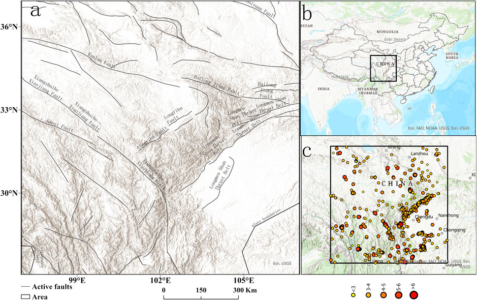
FIGURE 1. (A) is the location of the study area and the distribution of active faults, (B) illustrates that the study area is at the junction of Yunnan, Sichuan and Gansu in China, and (C) is the magnitude 3–8 earthquakes that have occurred in the study area in 2010-2020.
The earthquakes in our study extended geographically between 27° and 37°N and 97° to 107°E, and temporally between 2010 and 2020. The initial data we used were downloaded from the China Earthquake Networks Center (http://data.earthquake.cn). Usually, seismic studies use the magnitude-frequency distribution (MFD) to estimate earthquake rates and b-values according to the Gutenberg-Richter law (Gutenberg and Richter, 1949). Therefore, we performed a fundamental analysis of the above data, which should be identified using the “declustering process” for foreshocks, aftershocks, and seismic swarms.
Reasenberg’s algorithm determines mainshocks and aftershocks by constructing the time-space domain of the seismic sequence. The algorithm assumes an interaction zone centered on each earthquake, which is dynamically modeled with spatial (Rfact) and temporal (τmax) parameters (Reasenberg, 1985, 1969–1982). Given t>0, the probability of observing n earthquakes in the time interval [t, t+C] is given by Eq. 1 (Talbi et al., 2013)
Where Rfact is proportional to the source dimension, τmax is determined using a heterogeneous Poisson process for aftershocks, and ξ is the process that counts the number of aftershocks occurring in the time interval [t, t+τ]. where k, c, and p are positive constants representing the Omori law parameters.
We used the datasets required for investigation from the GEE, including the Moderate Resolution Imaging Spectroradiometer (MODIS), land surface temperature (LST and National Centers for Environmental Prediction (NCEP) Climate Forecast System Version 2 (CFSv2)) (Saha et al., 2011). Since there were missing values and cloud masks in the MODIS LST data, We used the CFSv2 coupled with temporal Fourier analysis (TFA) (Shiff et al., 2021). We obtained a continuous data set for our study to extract thermal infrared anomalies (TIR), which we called conLST on the GEE platform. Therefore, the daily nighttime conLST data for 2010–2020 used for our research were derived with 1 km spatial resolution.
The spatial resolution of the data determines the speed of the calculations and result is an issues that must be considered. Thereforce, in our study, we downscaled the spatial resolution from the initial spatial resolution of the ConLST data 1–50 km, according to a study of the effects of data at different spatial scales in seismic thermal anomalies by (Zhan et al., 2022).
We introduced coarse-graining into the TIR anomaly study to express the research process, was initially similar to adjusting the objective working distance in observing cells with a microscope. In this paper, we proposed a group of relative concepts, including coarse thermal infrared anomaly (CTIR) and refined thermal anomaly infrared (RTIR), which aimed to distinguish between anomalies obtained by anomaly detection techniques on time-series satellite data and thermal anomalies that may be linked to earthquakes. The method section includes (CTIR) extraction, RTIR detection, and evaluative criteria, looking at the advantages and disadvantages of the different methods.
Six anomaly detection methods were selected, including robust satellite techniques and interquartile range in statistical methods, wavelet transform in signal analysis, Kalman filter in filtering techniques, isolated forest in machine learning, and autoencoder in deep learning. Some of these have been widely used for seismic thermal anomaly extraction, while others are better methods for anomaly extraction techniques. In Table 1, the thresholds for various methods to determine CTIR and the choice of foundation are shown.
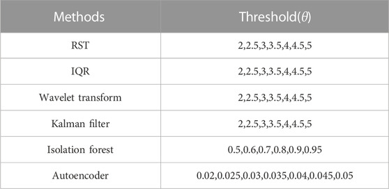
TABLE 1. The thresholds of the different methods.
The RST method was proposed by Tramutoli et al., 2013, and is based on satellite data rather than requiring ancillary data. Therefore, they can be entirely automated for operational real-time monitoring purposes (Eleftheriou et al., 2016). This method is based on multi-temporal analysis of a historical dataset of satellite observations acquired under similar observational conditions (Panda et al., 2007).
Because the RST was applied to thermal monitoring of earthquake-prone areas, TIR fluctuations were identified using the robust estimator of TIR anomalies (RETIRA). With different data sources and application environments, the index was eventually used as an absolutely local index of change in the environment (ALICE), which was computed as follows:
Where x,y represent the coordinates of the center of the ground resolution unit; and t is the time of the image,
Interquartile range (IQR) is a well-known method for anomaly detection, In descriptive statistics that represents a set of data arranged in order. Regarding seismic anomaly extraction, some researchers used the upper quartile and lower quartile to distinguish seismic anomalies from data (Liu et al., 2004; Akhoondzadeh, 2013). This method can be calculated using the following equations:
x, xupper, xlower, M, IQR and θ are parameters, higher bound, lower bound, median value, interquartile range and threshold for exceptions, respectively. The data parameters for the θ values are in Table 1.
The wavelet transform is a representation of the function time domain (spatial domain) and frequency (Gao et al., 2020). This was used as a data-mining tool to detect seismic anomalies with satellite data. Xiong et al. (2009) assessed several wavelet methods and selected two real continuous Daubechies Wavelets and Gaussian Derivative Wavelets (Xiong et al., 2009). In this study, we used the following to calculate conLST times series of earthquakes anomalies with respect to the temporal background field. Due to the variability of our data, the Daubechies 8D wavelet was applied to identify anomalies in the data. The low-frequency seasonal components and high-frequency noise were eliminated using the wavelet transform components.
Where, the a is the scaling factor, b is the location parameter, f is the complex conjugate of continuous wavelet function and f (t) is the time series under analysis.
The Kalman filter is a recursive solution to optimize the described systems in the state space. This is a collection of mathematics equations to optimize prediction equations using an estimation of state variables and minimization of error covariance (Saradjian and Akhoondzadeh, 2011). Multiple iterations of this calculation may obtain the best estimate. Assuming the state equation of the dispersive Kalman filter is as follows
Where
Isolation Forest proposed different types of model-based method that explicitly isolates anomalies rather than profiling normal instances. It has been widely used for anomaly extraction by (Liu et al., 2008). The method builds an ensemble of iTrees for a given dataset; anomalies are the instances with short average path lengths on the iTrees. Figure 2 provides a graph illustrating an example of the structure of n trees in the Isolation Forest.
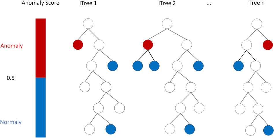
FIGURE 2. Graph example illustrating n trees of an isolate forest. It consists of two steps: step 1. isolation operations of data points using randomly constructed binary search tree; step 2. binary tree with the isolated point. The average path in red is the shortest, the earliest to be distinguished and is probably the outlier point.
In the article, isolation forests were used to extract CTIR, although they were seldom applied in earthquake precursor studies. The first (training) stage builds isolation trees using subsamples of the training set. The second (testing) stage passes the test instances through isolation trees to obtain an anomaly score for each instance.
Given a sample set of m instances, isolation forests gives the average path length of unsuccessful searches in Binary Search Tree as (Liu et al., 2012):
where n is the testing data size,m is the size of the sample set and H is the harmonic number, which can be estimated by H(i)=ln(i)+gamma, where gamma =.5772156649 is the Euler-Mascheroni constant.
Then, the anomaly scores s∈[0,1] of a test pixel x are defined as follows:
Where E (h(x)) is the average value of h(x) from a collection of iTrees. It is interesting to note that for any given instance x:if s is close to 1 then x is very likely to be an anomaly.if s is smaller than .5 then x is likely to be a normal value.if for a given sample all instances are assigned an anomaly score of around .5, then it is safe to assume that the sample does not have any anomaly.
Autoencoder is an unsupervised neural network that uses a neural network to generate a low-dimensional representation of a high-dimensional input. Autoencoder contains two main parts, encoder, and decoder (as shown in Figure 3). The encoder is used to discover a compressed representation of the given data, and the decoder is used to reconstruct the original input. During training, the decoder forces the autoencoder to select the most informative features, which are eventually saved in the compressed representation. The final compressed representation is in the middle coder layer. The difference between the original input vector x and the reconstructed vector z is called the reconstruction error
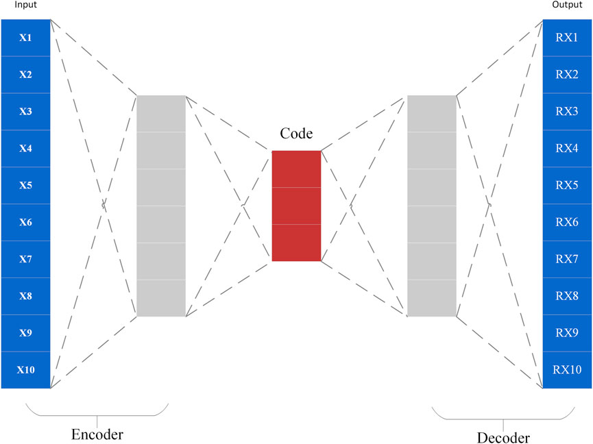
FIGURE 3. Graph example illustrating the encoder–decoder architecture of auto-encoder. First the input passes through the encoder, which is a fully-connected ANN, to produce the code. The decoder, which has the similar ANN structure, then produces the output only using the code. Final calculation of the original and reconstructed image as anomalies.
The encoder in Eq. 12 maps the input vector x to the hidden representation h using a non-linear affine mapping. The decoder in Eq. 13 maps the hidden representation h back to the original input space as a reconstruction by the same transformation as the encoder. The difference between the original input vector x and the reconstructed z is known as the reconstruction error, as in Eq. 14.
We obtained CTIR (i,α) from different methods, as shown in Section 2.3.1, to further obtain RTIR (i,α), the thermal anomaly possibly associated with the earthquake. In this section, we used the heating core proposed by (Zhang et al., 2021). To obtain RTIR (i,α). The model can remove noise that is unrelated to the seismic activity. We set the following limits: a series of time-space intensity (TSI) qualifications (Table 3), including the temporal persistence rule, spatial coverage rule, spatial persistence rule, and intensity persistence rule. All the CTIRs will be filtered with the above four rules, and the thermal infrared anomalies patches (CTIRs) are the remaining filtered results of CTIR (i,α), CTIR (i,α+1), and CTIR (i+1, β). CTIRs will be merged into TIR anomalies after the above rules are satisfied. The above extraction process depends on the parameters (θ, Areamin, Areamax, iou, T, D, M).
Next, we set a series of rules to determine the correspondence between earthquakes and RTIR anomalies in Table 2, including the temporal, distance, and magnitude rules. In the distance rule, we used the Euclidean distance as the shortest distance between the EQ (x, y, t, m), which is an event occurring at (x, y) on day t with magnitude m. RTIRn is less than or equal to D. To set parameters that consider different geological, meteorological, and environmental backgrounds. A training-test-validate approach was used to determine the best parameters for extracting TIR anomalies associated with earthquakes. We can obtain the optimal set of parameters and perform outlier extraction using the above parameters.
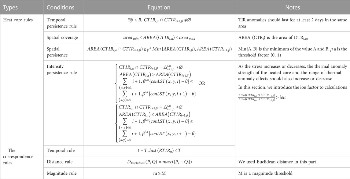
TABLE 2. The rules include rules for heating core model and rules for determining whether it is related to earthquakes.
In this part, we used P1, P2, and loss parameters to evaluate the effectiveness of different methods in CTIR anomalies in training–test–validation sets. P1 is the p-value for the false negative rate (FNR)-based alarms and P2 is the p-value for the positive predictive value (PPV)-based alarms. The significance level is a range of estimates for an unknown parameter, the 95% confidence level is the most commonly used to set. Therefore, the confidence interval for both P1 and P2 was set to .05 in this study, and loss (Eq. 15) is the evaluation score given by the 3D error diagram (Zhang et al., 2023; Zhang et al., 2021).
The w2 and w3 are weights measuring the relative costs of the y and z-axis. In this study, we set w1=w2 = w3 = 1. STCW is a space-time correlation window corrected by the Molchan diagram, weighted by the relative intensity (RI) index (Zechar and Jordan, 2008).
TP2 is the total number of earthquakes that correspond to RTIRs, FN is the total number of earthquakes that do not correspond to RTIRs.
TP1 is the total number of RTIRs that correspond to earthquakes, FP is the total number of RTIRs that do not correspond to earthquakes.
We used the training–testing–validating step to evaluate the best parameters from the 56,700 different vectors (Table 3). This can avoid mistaking normal seasonal warming for TIR anomalies to some extent. In the test step, the RTIRs data and earthquake catalog data from 2010.01.01 to 2012.12.13 will be used as the training dataset. At the same time, we performed the model on the validation set, which contains RTIRs data and earthquake catalog data from 2013.01.01 to 2016.12.31 in the test step and the data from 2017.01.01 to 2020.12.31 as the test dataset, called the validation step. The values of P1,P2, Loss are given in the above steps.
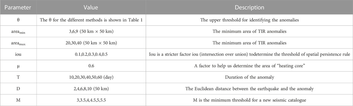
TABLE 3. Parameters to extract DTIRs and determine the correspondence between DTIRs and earthquakes.
We obtained the values of P1 and P2 for each group of parameters. We determined a threshold of .05 for P1 and P2 based on the method of confidence levels in statistics. The values of P1 and P2 have divided the given alerts into four classes based on the results in the training-test-validation step: Type I: P1≤.05 and P2≤.05, Type II: P1>.05 and P2≤.05, Type III: P1≤.05 and P2>.05, and Type IV: P1 > .05 and P2>.05. Type I, II, and III alarms effectively predict earthquakes, although type II and III are not optimal. Type IV alarms are not effective at predicting earthquakes.
The results of the original earthquake catalog and declustering data, analysis using R, are shown in Figure 4A, original; b, declustering). According to the earthquake catalog description, there were 1,140 seismic events in the region, and 899 events remained in the catalog after declustering, including seven with Ms>6. This produced a plot consisting of six subplots: Figures 4A, B show the spatial distribution of events, while Figures 4D–F, J–L plots show how the latitude (Figures 4D, J), longitude (Figures 4E, K) and magnitude of events change over time (Figures 4F, L), with two plots visually inspecting the completeness and time stationarity of the catalog. Figures 4C, I allows for cumulative magnitude to denote the number of events in the catalog with a magnitude greater than or equal to m (we selected m=3 in the article). The plot (Figures 4B, H) of log10(Nm) versus m shows the linear relation expected from the Gutenberg-Richter law. The plot of Nt versus t is linear during the considered study period. Despite this, a non-linear trend is evident over the time span 2010–01-01–2021-01-01 (4,018 days), probably due to the Mw=6.7 20 April 2013 Lushan earthquake occurrance. The Gutenberg–Richter law states that log10(Nm) = a—bm for some a and b, which is equivalent to assuming that m follows an exponential distribution (Roeloffs, 1988; Pulinets 2006).
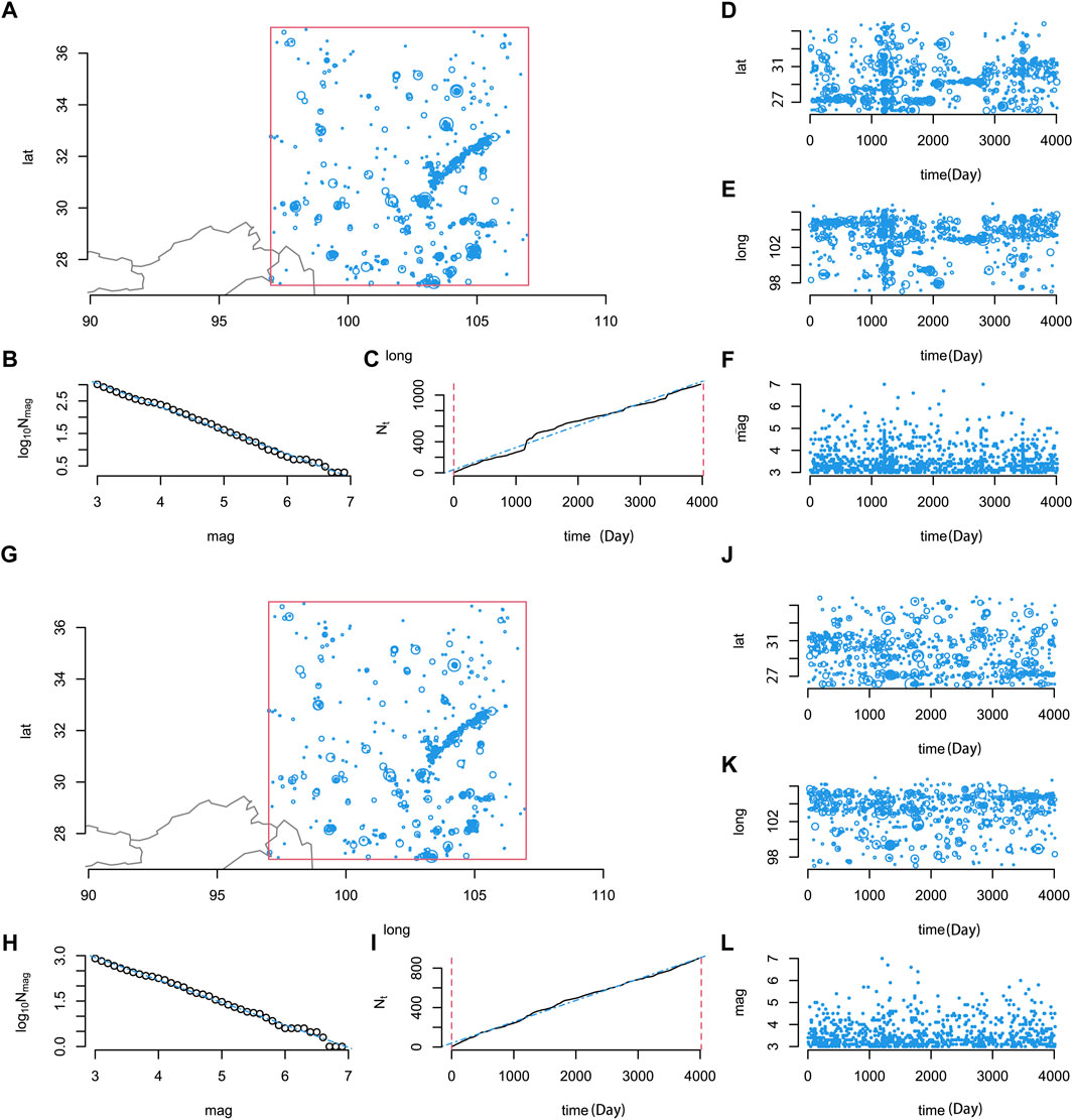
FIGURE 4. (A) is the original seismic catalog, (B) is the de-clustering seismic catalog. Location of epicenters (A, G), logarithm of frequency by magnitude (B, H), cumulative frequency over time (C, I) and latitude, longitude and magnitude against time (D–F), (J–L) of 1140 earthquakes with magnitude greater than or equal to 3 occurred between 2010-01-01 and 2021-01-01 in Sichuan and its vicinity (27◦–37◦N and 97◦–107◦E), extracted from the China Earthquake Networks Center (http://data.earthquake.cn). The plots are created by R.
We used six different methods to extract CTIRs in Section 2.3.1 without filtering by the rules (Table 2) that effectively predict earthquakes. First, we used alarm types to evaluate the advantages and disadvantages of the different methods, which was carried out by calculating the alarm types generated by 56,700 sets of parameters during the training–test–validation process.
In the training steps, we focused on the number of type alarms generated in the 56,700 parameters set. The number of alerts of each type was calculated as a ratio of the total alert data volume. The results indicate that (Figure 5A) the autoencoder and isolation forest methods produced more type-Ⅰ alarms than the other methods, and the Kalman filter method was the worst performer. Among the type Ⅰ alarms, the significant percentages were AE and IF, accounting for 58.49% and 16.37% of the total. Although type II and type III alarms are unlike type I alarms, which are effective for predicting earthquakes from the FNR and PPV perspective, they are still counted and analyzed. Therefore, other alert types were given in proportion to the ones generated by the above methods (Figure 5A). Below we showed the number of alerts with type Ⅰ: AE>IF> IQR>RST>KF>WT.
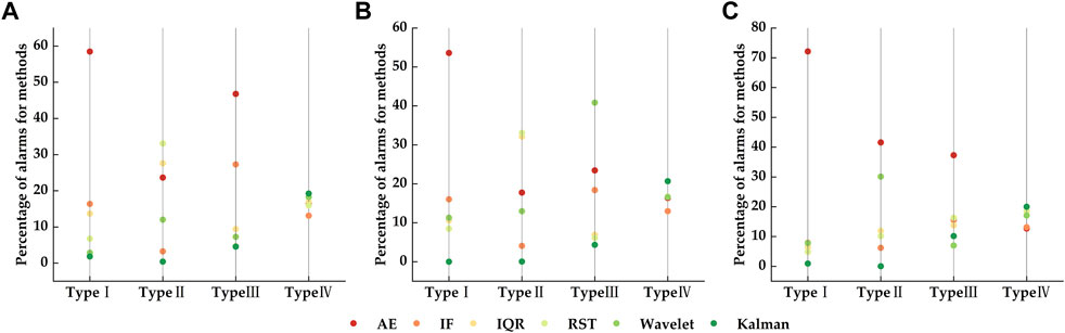
FIGURE 5. The result of type alarms. (A–C) represent the ratio of each type of alert generated by different methods to the overall training (A), test (B) and validation (C) steps. (A–C) display relatively consistent features; warm and cold color scatter represent the proportion of alerts of that type generated by the method, with warm colors representing the proportion and cold colors the opposite.
To test the effect of the 56,700 sets of parameters obtained in the training step, we filtered the above parameters in CTIRs and earthquake catalogs from 2013 to 2016 with the heat core. The plots (Figure 5B) were also presented below regarding the type of alert. In test step results, the AE and IF methods, which generated the most alerts, remained optimal. Among the type Ⅰ alarms, the significant percentages were AE and IF, accounting for 53.6% and 16.02% of the total. Below, we give the number of alerts for the type Ⅰ method from major to minor: AE>IF>WT>IQR>RST>KF.
We obtained the alert types corresponding to 56,700 sets of parameters through a training–test steps, which led us to explore the strength of each method. However, in the paper, we should add validation step to explore the impact of the method. In terms of the type Ⅰ alarm, the proportion of the number of alarms for AE are 72.14%. Below, we provide the number of alerts for the type Ⅰ method from greater to lesser: AE>IF> WT> IQR>RST>KF (Figure 5C). Overall, the AE and IF methods generated more data for type Ⅰ alerts in the training–test–validation steps. In the following, we will further determine the parameters of each method corresponding to type Ⅰ alarms and obtain the optimal parameters for each method.
Each parameter produces P1 and P2 values at each step, so three P1 and P2 values should be available for each parameter. In Section 3.2, we obtained the parameters of type Ⅰ alarms (P1≤.05,P2≤.05) in each method’s training–test–validation steps. To further evaluate the various methods for refining the extraction of infrared thermal (RTIR) anomalies, the optimal parameters of each method were searched.
In order to distinguish between the three types and visualisation, we labeled the corresponding D1,D2, D3 with the red, yellow and blue signs presented in Figure 6. Loss is the weighted sum of FDR, FNR and STCW, the lower the Loss is the better the alarms are. Only Loss values that pass the P1 and P2 tests are significant, D1 corresponds to three steps of Loss values (Losstrain, Losstest, Lossvalidation), D2 has two Loss values (Losstrain, Losstest) and D3 has one Loss value (Losstrain). Obviously, the corresponding Loss values are generated in the training-test-valiadtion phase. The Lossm is the mean value of the above three session loss value. Finding the optimal set (θ, Areamin, Areamax, iou, T, D, M) of parameters is determined by the alert types and Loss values we have described above. Only the parameters of AE and IF methods resulted in D1, where it passed significance in the training–test–validation steps for both P1, P2. In terms of the autoencoder (Figure 6A), the symbol marked in red is the result with the lowest Lossm=.754. The best parameter set of D1 (θ=.015, Areamax=30, Areamin=9, iou=.2, T=10, D=10, M=3) was tested in test and validation steps. The result of the next steps (in test step: PPV = 72.4%, FNR = 44.4%, STCW =45.1%, P1=

FIGURE 6. The result of the best parameters for methods. (A–F) represent the optimal parameters of each method to the overall training step [(A): AE, (B) IF, (C) IQR, (D) WT, (E) RST, (F) Kalman]. The x-axis and y-axis of the diagram are the fraction of space-time occupied by alarms and the FNR, respectively, and the z-axis is the FDR (FDR= 1-PPV). The symbol marked by red, yellow, and blue are the parameter sets with the lowest Lossm.
The yellow sign in Figures 6C–E means that they are the best parameters of type D2 for the IQR, WT and RST methods. They indicate that P1 and P2 passed the significance test in the training–test steps (P1≤.05,P2≤.05), which are the relative optimal parameters in the method. For IQR methods, the best parameter is θg = (θ=2, Areamax=40, Areamin=3, iou=.3, T=10, D=10, M=3) with the lowest Lossm= .842 ((in test step: PPV = 64.6%, FNR = 7.59%, STCW = 76.7%, P1= .0282 and P2 = .000173). The optimal parameters of the two remaining methods can be described as follows: WT = (θ=4.5, Areamax=30, Areamin=6, iou=.3, T=10, D=10, M=3) with the lowest Lossm= .677 (in test step: PPV = 61.3%, FNR = 45.4%, STCW =73.8%, P1=.001671 and P2 =.003098); RST= (θ=2, Areamax=20, Areamin=3, iou=.4, T=10, D=10, M=3) the lowest Lossm= .809 (in test step: PPV = 67.3%, FNR = 15.9%, STCW = 70.4%, P1= .0181 and P2 = .00000622). In the validation step, the alert types for the different methods are type II(IQR: P1=.999, P2=.000258,WT: P1=.012, P2=.00014, RST: P1=.99, P1=.0000429), which are effective for predicting earthquakes from the view of FNR. People can effectively avoid as many false alarms as possible if they reducing risk according to these alarms.
The optimal parameter of type D3 is indicated by the blue symbol (Figure 6F) for the Kalman filter method with the lowest Lossm= .833. The best method is θg = (θ=2, Areamax=20, Areamin=3, iou=.4, T=10, D=20, M=5, in the training step: PPV = 29.5%, FNR = 42.9%, STCW = 83.3%, P1= .01048 and P2 = .00254). The alert types in the test step are type IV(P1=.842, P2=.879). In the validation step, The alert types are type III(P1=.00365, P2=.0998).
The alarm type is our main concern for the above results and indicates the best parameter for each step. Therefore, we have plotted Figure 7 to indicate the loss values at each stage for the different methods. As shown in Figure 7, the optimal parameters fall into the D1 of AE and IF methods which means that the optimal parameters pass both the P1 and P2 significance tests in the training-test-validation step. The other three methods are optimal parameters for the D2 class including RST, IQR and WT. These approaches best parameters produce intersection sets in the training-testing phase. Only the optimal parameters of the KF is in the training phase. We obtained the optimal set of parameters for the minimum Lossm. They can be found in Table 4 for each method. It can be observed that the M and D parameters of the optimal parameters are relatively uniform across the six methods. RTIR anomalies are generated from the above parameters as the basic parameters for subsequent analysis results. Results of TIR anomalies.
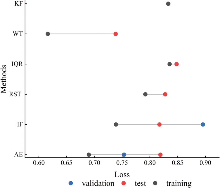
FIGURE 7. The result of the Loss values for six methods. (AE,IF,RST,IQR,WT,KF). The x-axis is the Loss value and the y-axis represents the different methods. Three colors correspond to the training-test-validation steps (red is the training phase, blue is the test phase and black is the validation phase).
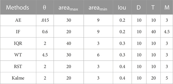
TABLE 4. The optimal parameters for each method.
In Section 3.3, we obtained the optimal parameters for each method to extract TIR anomalies correlated with a statistically significance to the seismic activity. We extracted RTIR anomalies using the above parameters based on the heating core rule in our other work. To better compare the results generated by the different steps of the workflow, we have named the TIR exceptions corresponding to the steps CTIR anomlies, RTIR anomlies. The ‘heating core’ rules are effective in eliminating these TIR-anomalous signals, which are unlikely to be associated with earthquakes. We compared the number of anomalies for each method between unfiltered suspected TIR anomalous signals and filtered suspected TIR anomalous signals. Coarse-graining will be further discussed in this section.
To study the filtering effect of the non-seismic anomalies of the heated kernel model on different methods, we showed the number of day with thermal anomalies for RTIR and CTIR, representing anomalies with filtering before and after. The average CTIR anomalous signal number of the day, derived using the AE method, is 2731, while the average RTIR abnormal signatures number of the day, derived using the AE method, is 1021. The abnormal days of CTIR anomalous signatures for the IF method are 1125, compared to 2961 for the RTIR anomalous signals. The RST and IQR methods indicate that the number of abnormal days in the RTIR session is 3677 and 2524, while in CTIR, the results are strongly filtered, and the number is 1523 and 1040. The 3002 days generated RTIR anomalies that consisted of many non-seismic anomalous factors, extracted under the WT method; meanwhile, 1,168 days of anomalies were identified as CTIR unusual signatures. Only 225 days presented the RTIR anomaly, which is apparently less relative to the 11-year time interval derived by the Kalman filter method based on the CTIR being 3967. As a result, we can see the heating core rules that we set for different ways, which can effectively filter non-seismic anomalous signals. The identification rules significantly reduce the number of TIR anomalies in the coarse-graining process (from RTIR to CTIR anomalies).
In the above, we discussed the number of anomalous days to describe the filtering effect of heating cores on different methods. We designed the process to study the coarse-grained seismic thermal anomaly, which sets a series of time, spatial, and intensity conditions based on the heating core model to obtain the CTIR anomalies from RTIR signals. In Figure 8, we show the spatial distribution of the proportion of RTIR and CTIR anomaly frequencies and the associated proportions generated by each method in 2010–2020. Figures 8A–E corresponds to each method, while each left, middle, and right subplot represents RTIR anomalous and CTIR signals, respectively, showing the ratio of the frequency of removed TIR anomalous signals to the frequency of RTIR anomalies. As shown in Figure 8 a-left, for the unfiltered results of AE method results, the frequency of the RTIR signal in the middle is much lower than that in the west, east, north, and south. In the CTIR step, Figure 8 a-middle shows that the signal frequency of the results were significantly lower throughout the study area, and the frequency was highest in the northwest corner, followed by the north and south, and lowest in the center. As shown in Figure 8A-left, 90% of RTIR signals were removed in the middle, while in the north and south, about 80% RTIR signals were removed. Similar descriptions are used to express the spatial distribution of TIR anomalies for different methods, including RTIR, CTIR, and proportion. The left and middle panels of Figure 8B show a similar spatial distribution, with high-frequency anomalies in the four corners and many banded anomalous frequencies in the middle using the IF method. The overall anomaly removal rate is 90%. The TIR anomalies extracted by RST and IQR show the same spatial distribution characteristics in Figures 8C, D. As the left panels show, the study area was covered by RTIR anomalies, where the highest frequency of anomalies occurred in the southeast corner. From the RTIR to CTIR steps, the TIR anomalies in the southwest corner were more reserved and showed banding under the RST method. This process still removes 70%–80% of the RTIR signal, even though 20%–30% of the anomalies are retained in the southwest. The RTIR anomalies extracted by the WT method are mainly distributed in the southeast, as shown in Figure 8. e-left. High-frequency anomalies appear in the southwest after filtering the anomalies in Figure 8E-middle. The filtration percentage is still between 10% and 20%, which means that most of the RTIR is removed with Figure 8E-left. The Kalman filter method contributes the highest anomaly frequency values, with high values distributed in the south-east in Figure 8F-left. The filtered result is similar to the previous method in Figure 8F-middle.
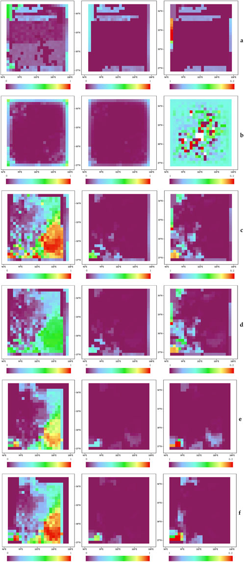
FIGURE 8. The result of frequency of the RIT and CTIR anomalies generated by each method in 2010–2020 [(A): AE, (B) IF, (C) IQR, (D) RST:, (E) WT, (F) Kalman], The x-axis represents the longitude; the y-axis represents the latitude. Subplot-left is the frequency of RIR Signal of the whole area, while Subplot-center is the frequency of CTIR Signal. Subplot-right is the ratio of the frequency of removed TIR anomalous signals from RTIR to the frequency of CTIR results (ratio = (TIRRTIR-TIRCTIR)/TIRRTIR).
In Section 3.4, we analyzed the spatial anomaly frequency distribution of TIR anomalies using each method. There are anomalies in the southwest region, extracted by the different techniques in Figure 8. Meanwhile, the southwest region is the junction zone of plate tectonics between the India Plate and Gansu–Qinghai–Tibetan Plate, as shown in Figure 1. In the precursor study, Ishibashi et al. divided the LST anomalies into tectonic precursor types, which are a link in a chain of particular local tectonism in each individual area preceding the earthquake (Molchan, 1990). Therefore, we further determined the advantages of the above methods using the relationship between the above RTIR anomaly and active fracture zones, stress distribution and seismic belts. Several active fracture zones exist, such as the Xianshui River–Anning River faultline and the Longmenshan faultline. As shown in Figure 9-left, the stress distribution is similar to the fault belt.
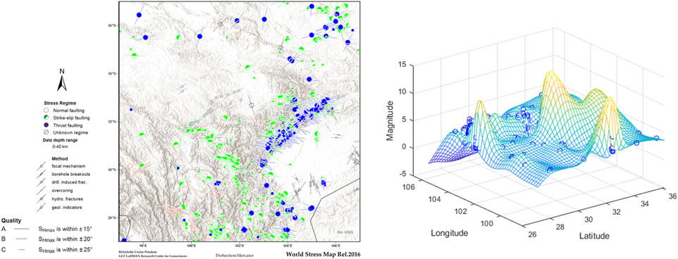
FIGURE 9. Left subplot is stress map of the study area (the data are provided by http://www.world-stress-map.org/); right subplot is 3D seismic belts–earthquake distribution map; there are three seismic belts, including the Western Yunnan belt, Western Yunnan belt, and Anning river belt.
The CTIR thermal anomalies extracted show no tectonic features using the AE method since the frequency anomalies distribution of the extracted multi-year did not correspond to stresses, seismic belts and fracture zones. Surprisingly, the CTIR anomaly frequency spatially corresponded to the Xianshui River–Anning River rift zone extracted by the IF method, but its frequency is lower in value between 300 and 400 days. For the first time, isolated forests were used for seismic thermal anomaly extraction, and the results suggest that this is a promising method. The spatial distribution of the RTIR anomaly frequencies extracted by RST and IQR is similar to those mentioned previously. When we consider the tectonic factors, we found that the RTIR anomaly frequency extracted by RST is consistent with the stress distribution characteristics near the fracture zone. RTIR anomalies are not correlated with stress, the active fault distribution extracted by the IQR method, even though the CTIR results are similar to those extracted by the RST method. The RTIR anomaly frequency distribution has a block shape, which is not relative to the constructive factors extracted using the WT method. The Kalman filter method produced lower quality results because no TIR anomaly was corresponding to the physical/geographical factors.
Finally, we attempted to present a comparative summary of each method based on the previous results. In the RTIR result, the Kalman filter method produced a higher frequency of TIR anomalies compared to other methods. This result is consistent with the study that showed that the Kalman filter method performed best, with the most extreme and erratic variations in the LST (Molchan, 1991). In the CTIR step, AE and IF showed the optimal parameters and the type of alert, while the poorly performing method was the Kalman filter. The IQR and RST methods are robust, as shown in both RTIR and CTIR results, including the RTIR results showing a high frequency of anomalies, and the optimal parameters in CTIR are the category II optimal parameters. Type III optimal parameters indicate a weak statistical correlation between anomalies and earthquakes under the heated core filtering rule. We introduced tectonic information to view the CTIR anomaly and determined the correlation between the anomalies and earthquakes. By integrating the relationship between the RTIR anomalous signal and the constructive factors, we found that RST maintains a relatively favorable anomaly frequency and spatial distribution. It is worth further examining the IF method because it produces RTIR anomalies that fit the space characteristics of the construct distribution. Therefore, we ranked the advantages of the following methods in different steps, according to the results:
The current LST products are limited, due to missing data due to pixels that are overcast by clouds. To solve this problem, we implemented NCEP and LST data to fill in the missing data based on the GEE platform. Therefore, we used conLST data derived from a Google Earth Engine with Temporal Fourier Analysis (TFA) as the experimental data for anomaly extraction, which can generate daily, daytime and nighttime data. Regarding the temporal resolution, the daily nighttime data are used to exclude the conLST data covered by the cloud. To reduce the efforts of computational and anomaly continuity, we resampled the conLST data with 50 km spatial resolution. We declustered the seismic catalog using the Reasenberg method to separate earthquakes in the seismicity catalog into independent and dependent earthquakes.
There are several methods for extracting TIR precursors of earthquakes more than these six methods mentioned in our article. We summarize the current types of TIR precursor extraction methods using the meta-analysis literature methods, including mathematical/statistical methods, wavelet transforms, filtering methods, machine learning and deep learning. However, many classical methods and intelligent approaches are not used, for example autoregressive integrated moving average (ARIMA), artificial neural network (ANN), support vector machine (SVM) (Akhoondzadeh, 2013), Eddy field method and Z-score method. On the other hand, many methodological improvements were not considered and implemented, such as the wavelet transform, which can be improved in several ways. At the same time, there is no more in-depth study of machine learning and deep learning methods like CNN, LSTM and random forest.
The threshold effect continues throughout our research. We used a survey of the literature or the principles of anomaly extraction methods to determine the thresholds for each session. Thus, there are problems: the parameters may be absent or inherently incorrect, as obtained from the publications. The threshold θ is slightly different for each method in table 2-1. For example, AE and IF have no thresholds for reference as there is no literature on their application to seismic anomaly extraction. Therefore we can only define the threshold based on the characteristics of the method (e.g. .5 for IF as an important exception threshold). Only the RST threshold has a lot of thresholds in long-term studies for the other four methods.
Many works have been conducted to statistically analyze the relationship between TIR anomalies and earthquakes. However, there are still doubts regarding the correlation between earthquakes and TIR precursors. Recently, Zhang et al., 2021 provided strong statistical evidence of TIR anomalies and earthquakes by constructing the heating core model (Zhang et al., 2021). To filter thermal anomalies in CTIR that are unrelated to earthquakes, we used training–testing–validation steps to set many parameters to extract RTIR anomalies and determine the correspondence between TIR precursors and earthquakes in the next step (train–testing steps in the original study). We obtained the optimal parameters for each method by the above steps. In our research, the optimal global parameters are discussed more, ignoring the most local parameters that can be extracted under the characteristics of the study area. The spatial variable parameters will be studied in the future to better understand the mechanism of TIR anomalies and earthquakes.
Although we used statistical methods to evaluate the influence of TIR anomaly extraction, tectonic background factors were not quantified and statistically analysed in this study. For example, Yang et al., 2022 studied the relationship between quantified bright temperature anomalies and stress. (Qi et al., 2021). showed the evolution process of positive microwave brightness temperature (MBT) anomalies basically reflected the joint effect of crustal stress and seismogenic environment and regional coversphere on surface microwave radiation. Therefore, Extending the heating core model may be an important tool to improve mechanistic understanding with additional physical/geological contexts.
Seismicity declustering is widely used to separate an earthquake catalog into foreshocks, mainshocks, and aftershocks in seismology (Talbi et al., 2013). Many declustering methods have been proposed over the years such as Reasenberg, Window Methods, Stochastic Declustering et, al. There is the doubt whether declustering the seismic catalog when we perform a correlation study between TIR anomalies and the earthquake. In fact, declustering implies the extraction of mainshocks of higher magnitude than foreshocks and aftershocks. Therefore, associating the anomaly with the largest magnitude earthquake may imply relating it to the mainshock. (Marchetti et al., 2022). found is beneficial to extract possible seismo-anomalies after comparing the effect of the presence or absence of declustering. Of course it needs further research to discuss the necessity of declustering.
This study still has a lot of limitations. There are many parameter settings in multiple study sessions, but the selection of parameters did not take more factors into account. Although we have demonstrated the relationship between anomalies and earthquakes using statistical analysis, the mechanism of TIR seismic anomalies is yet unclear. In order to set the parameter for each step, we use information from the literature. However, we admit that the existing literature is descriptive rather than exploratory. We use a training-test-validation approach to obtain the optimal parameters, but the original set of parameters still affects our results. It is well known that the mechanism of TIR precursors has never been determined, However, There are theories such as p-hole activation theory, remote sensing rock mechanics, and seismo-ionosphere coupling theory (Saraf et al., 2009; Freund, 2011). Therefore, from a statistical perspective, we can only determine whether the anomaly is related to the earthquake. The improvements from MD were applied in research, but the 3D error diagram is still is under review (Zhang et al., 2023). Threshold questions about each method of quantifying the impact of parameters remains unresolved. Perhaps it can be resolved in future study.
In this paper, we proposed an evaluation process used to compare the effectiveness of TIR anomaly extraction methods. As shown in Figure 10, the process was divided into three parts: CTIR anomaly extraction, RTIR anomaly extraction and constructive factor filtering. Eleven years (2010–2020) of daily conLST data, acquired from GEE, were used to identify LST fluctuations relationship with M≥3 that earthquakes occurred in the study area over the same period. Multiple parameters or sets of parameters were used in various parts of the research to avoid the mistakes caused by one parameter. Therefore, we employed the training–test–validation steps to obtain the optimal parameters and determined the merits of this method, determine from the optimal parameter type. To verify and improve the evaluation process that we have proposed, we selected some previously studied methods (RST, IQR, WT, KF), and methods that have not been used for seismic thermal anomaly extraction (IF, AE).
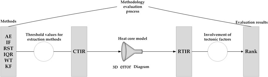
FIGURE 10. TIR anomaly method evaluation flow chart.
The results of our experiments are as follows:
• The heating core model can effectively improve the detection of TIR anomalies caused by earthquakes, and remove to some degree the TIR anomalies not caused by earthquakes. At the same time, the heated core model plays a filtering role for different anomaly extraction methods This can establish a strong statistical relationship between TIR anomalies and earthquakes.
• The ranking is given below for each step regarding the merits of the method through our proposed evaluation process: In the RTIR step: Kalme filter>RST>IQR>WT>AE>IF; in the CTIR step: CTIR: AE>IF>RST>IQR>WT>Kalme filter; the results after considering the constructive factors: RST>IF>IQR>WT>Kalme filter>AE. We introduced tectonic factors to avoid the non-causal correlation problem, although a high statistical correlation was generated between the TIR anomalies and the earthquake in the previous two steps.
• No method that can completely extract the thermal anomalies associated with earthquakes. The process provides a multifaceted evaluation of the extraction method, including the number of anomalies, statistical relationships, and physical/geographical factors.
The original contributions presented in the study are included in the article/Supplementary Material, further inquiries can be directed to the corresponding author.
For Conceptualization, PW; Software, PW; Supervision, QM; Validation, LZ; Visualization, MA; XH Writing—original draft, PW; Writing—review and editing, QM and CZ. All authors have read and agreed to the published version of the manuscript.
This research was supported by: the National Natural Science Foundation of China Major Program, grant number 42192580,42192580; the National Key Research and Development Program of China: 2019YFC1509202; the National Natural Science Foundation of China, grant number 42201384; the National Key Research and Development Program of China: 2020YFC0833100.
The authors declare that the research was conducted in the absence of any commercial or financial relationships that could be construed as a potential conflict of interest.
All claims expressed in this article are solely those of the authors and do not necessarily represent those of their affiliated organizations, or those of the publisher, the editors and the reviewers. Any product that may be evaluated in this article, or claim that may be made by its manufacturer, is not guaranteed or endorsed by the publisher.
Akhoondzadeh, M. (2013). A comparison of classical and intelligent methods to detect potential thermal anomalies before the 11 August 2012 Varzeghan, Iran, earthquake (Mw = 6.4). Nat. Hazards Earth Syst. Sci 13, 1077–1083. doi:10.5194/nhess-13-1077-2013
Bakun, W. H., Aagaard, B., Dost, B., Ellsworth, W. L., Hardebeck, J. L., Harris, R. A., et al. (2005). Implications for prediction and hazard assessment from the 2004 Parkfield earthquake. Nature 437, 969–974. doi:10.1038/nature04067
Bao, Z., Yong, S., Wang, X., Yang, C., Xie, J., and He, C. (2021). Seismic reflection analysis of AETA electromagnetic signals. Appl. Sci. 11, 5869. doi:10.3390/app11135869
Bhardwaj, A., Singh, S., Sam, L., Joshi, P. K., Bhardwaj, A., Martín-Torres, F. J., et al. (2017). A review on remotely sensed land surface temperature anomaly as an earthquake precursor. Int. J. Appl. Earth Observation Geoinformation 63, 158–166. doi:10.1016/j.jag.2017.08.002
Blackett, M., Wooster, M. J., and Malamud, B. D. (2011). Exploring land surface temperature earthquake precursors: A focus on the Gujarat (India) earthquake of 2001: Earthquake land temperature study. Geophys. Res. Lett. 38. doi:10.1029/2011GL048282
Cambiotti, G., Bordoni, A., Sabadini, R., and Colli, L. (2011). GRACE gravity data help constraining seismic models of the 2004 Sumatran earthquake. J. Geophys. Res. 116, B10403. doi:10.1029/2010JB007848
Chen, H., Xie, Q., Dai, B., Zhang, H., and Chen, H. (2016). Seismic damage to structures in the M s6.5 Ludian earthquake. Earthq. Eng. Eng. Vib. 15, 173–186. doi:10.1007/s11803-016-0314-4
Eleftheriou, A., Filizzola, C., Genzano, N., Lacava, T., Lisi, M., Paciello, R., et al. (2016). Long-term RST analysis of anomalous TIR sequences in relation with earthquakes occurred in Greece in the period 2004–2013. Pure Appl. Geophys. 173, 285–303. doi:10.1007/s00024-015-1116-8
Eleftheriou, A., Filizzola, C., Genzano, N., Lacava, T., Lisi, M., Paciello, R., et al. (2021). Correction to: Long-term RST analysis of anomalous TIR sequences in relation with earthquakes occurred in Greece in the period 2004-2013. Pure Appl. Geophys. 178, 1529. doi:10.1007/S00024-021-02692-4
Filizzola, C., Corrado, A., Genzano, N., Lisi, M., Pergola, N., Colonna, R., et al. (2022). RST analysis of anomalous TIR sequences in relation with earthquakes occurred in Turkey in the period 2004–2015. Remote Sens. 14, 381. doi:10.3390/rs14020381
Freund, F. (2011). Pre-earthquake signals: Underlying physical processes. J. Asian Earth Sci. 41, 383–400. doi:10.1016/j.jseaes.2010.03.009
Gao, J., Wang, B., Wang, Z., Wang, Y., and Kong, F. (2020). A wavelet transform-based image segmentation method. Optik 208, 164123. doi:10.1016/j.ijleo.2019.164123
Geiß, C., and Taubenböck, H. (2013). Remote sensing contributing to assess earthquake risk: From a literature review towards a roadmap. Nat. Hazards 68, 7–48. doi:10.1007/s11069-012-0322-2
Genzano, N., Filizzola, C., Paciello, R., Pergola, N., and Tramutoli, V. (2015). Robust Satellite Techniques (RST) for monitoring earthquake prone areas by satellite TIR observations: The case of 1999 Chi-Chi earthquake (Taiwan). Journal of Asian Earth Sciences 114, 289–298. doi:10.1016/j.jseaes.2015.02.010
Genzano, N., Filizzola, C., Hattori, K., Pergola, N., and Tramutoli, V. (2021). Statistical correlation analysis between thermal infrared anomalies observed from MTSATs and large earthquakes occurred in Japan (2005–2015). J. Geophys Res. Solid Earth 126, 108. doi:10.1029/2020JB020108
Gutenberg, B., and Richter, C. (1949). Seismicity of the Earth and associated phenomena. Princeton University Press. Available at: https://books.google.com.hk/books?id=BEVaXVPHstQC.
Hassanien A. E., and Darwish A. (Editors) (2021). Machine learning and big data analytics paradigms: Analysis, applications and challenges (Cham: Springer International Publishing). doi:10.1007/978-3-030-59338-4
Hayakawa, M. (2018). “Earthquake precursor studies in Japan,” in Geophysical monograph series. Editors D. Ouzounov, S. Pulinets, K. Hattori, and P. Taylor (Hoboken, NJ, USA: John Wiley & Sons), 7–18. doi:10.1002/9781119156949.ch2
Hayakawa, M., Hobara, Y., Ohta, K., Izutsu, J., Nickolaenko, A. P., and Sorokin, V. (2011). Seismogenic effects in the ELF schumann resonance band. Trans. Inst. Electr. Eng. Japan.A 131, 684–690. doi:10.1541/ieejfms.131.684
Hayakawa, M., Hobara, Y., Rozhnoi, A., Solovieva, M., Ohta, K., Izutsu, J., et al. (2013). The ionospheric precursor to the 2011 march 11 earthquake based upon observations obtained from the Japan-pacific subionospheric VLF/LF network. Terr. Atmos. Ocean. Sci. 24, 393. doi:10.3319/tao.2012.12.14.01(aa)
Hinton, G. E., and Salakhutdinov, R. R. (2006). Reducing the dimensionality of data with neural networks. Science 313, 504–507. doi:10.1126/science.1127647
Jiao, Z.-H., Zhao, J., and Shan, X. (2018). Pre-seismic anomalies from optical satellite observations: A review. Nat. Hazards Earth Syst. Sci. 18, 1013–1036. doi:10.5194/nhess-18-1013-2018
Jiao, Z., and Shan, X. (2022). Pre-seismic temporal integrated anomalies from multiparametric remote sensing data. Remote Sens. 14, 2343. doi:10.3390/rs14102343
Jin, S., Li, Z. C., and Park, P.-H. (2006). Seismicity and GPS constraints on crustal deformation in the southern part of the Korean Peninsula. Geosci. J. 10, 491–497. doi:10.1007/BF02910442
Jin, S., Park, P., and Zhu, W. (2007). Micro-plate tectonics and kinematics in Northeast Asia inferred from a dense set of GPS observations. Earth Planet. Sci. Lett. 257, 486–496. doi:10.1016/j.epsl.2007.03.011
Jin, S., Zhu, W., and Afraimovich, E. (2010). Co-seismic ionospheric and deformation signals on the 2008 magnitude 8.0 Wenchuan Earthquake from GPS observations. Int. J. Remote Sens. 31, 3535–3543. doi:10.1080/01431161003727739
Jin, S., Jin, R., and Liu, X. (2019). GNSS atmospheric seismology: Theory, observations and modeling. Singapore: Springer Singapore. doi:10.1007/978-981-10-3178-6
Liu, J. Y., Chuo, Y. J., Shan, S. J., Tsai, Y. B., Chen, Y. I., Pulinets, S. A., et al. (2004). Pre-earthquake ionospheric anomalies registered by continuous GPS TEC measurements. Ann. Geophys. 22, 1585–1593. doi:10.5194/angeo-22-1585-2004
Liu, F. T., Ting, K. M., and Zhou, Z.-H. (2008). “Isolation forest,” in Proceeding of the 2008 Eighth IEEE International Conference on Data Mining (Pisa, Italy: IEEE), 413–422. doi:10.1109/ICDM.2008.17
Liu, F. T., Ting, K. M., and Zhou, Z.-H. (2012). Isolation-based anomaly detection. ACM Trans. Knowl. Discov. Data 6, 1–39. doi:10.1145/2133360.2133363
Marchetti, D., De Santis, A., Campuzano, S. A., Zhu, K., Soldani, M., D’Arcangelo, S., et al. (2022). Worldwide statistical correlation of eight years of swarm satellite data with M5.5+ earthquakes: New hints about the preseismic phenomena from space. Remote Sens. 14, 2649. doi:10.3390/rs14112649
Molchan, G. M. (1990). Strategies in strong earthquake prediction. Phys. Earth Planet. Interiors 61, 84–98. doi:10.1016/0031-9201(90)90097-H
Molchan, G. M. (1991). Structure of optimal strategies in earthquake prediction. Tectonophysics 193, 267–276. doi:10.1016/0040-1951(91)90336-Q
Molchanov, O. A., Kopytenko, Yu. A., Voronov, P. M., Kopytenko, E. A., Matiashvili, T. G., Fraser-Smith, A. C., et al. (1992). Results of ULF magnetic field measurements near the epicenters of the Spitak (M s = 6.9) and Loma Prieta (M s = 7.1) earthquakes: Comparative analysis. Geophys. Res. Lett. 19, 1495–1498. doi:10.1029/92GL01152
Ouzounov, D., Bryant, N., Logan, T., Pulinets, S., and Taylor, P. (2006). Satellite thermal IR phenomena associated with some of the major earthquakes in 1999–2003. Phys. Chem. Earth Parts A/B/C 31, 154–163. doi:10.1016/j.pce.2006.02.036
Ouzounov, D., Liu, D., Chunli, K., Cervone, G., Kafatos, M., and Taylor, P. (2007). Outgoing long wave radiation variability from IR satellite data prior to major earthquakes. Tectonophysics 431, 211–220. doi:10.1016/j.tecto.2006.05.042
Panda, S. K., Choudhury, S., Saraf, A. K., and Das, J. D. (2007). MODIS land surface temperature data detects thermal anomaly preceding 8 October 2005 Kashmir earthquake. Int. J. Remote Sens. 28, 4587–4596. doi:10.1080/01431160701244906
Parrot, M., and Li, M. (2018). “Statistical analysis of the ionospheric density recorded by the DEMETER satellite during seismic activity,” in Geophysical monograph series. Editors D. Ouzounov, S. Pulinets, K. Hattori, and P. Taylor (Hoboken, NJ, USA: John Wiley & Sons), 319–328. doi:10.1002/9781119156949.ch18
Pulinets, S. (2006). Space technologies for short-term earthquake warning. Advances in Space Research 37, 643–652. doi:10.1016/j.asr.2004.12.074
Qi, Y., Wu, L., Ding, Y., Liu, Y., Chen, S., Wang, X., et al. (2021). Extraction and discrimination of MBT anomalies possibly associated with the Mw 7.3 maduo (Qinghai, China) earthquake on 21 may 2021. Remote Sens. 13, 4726. doi:10.3390/rs13224726
Qin, K., Wu, L. X., De Santis, A., and Cianchini, G. (2012). Preliminary analysis of surface temperature anomalies that preceded the two major Emilia 2012 earthquakes (Italy). Ann. Geophys. 55, 40. doi:10.4401/ag-6123
Reasenberg, P. (1985). Second-order moment of central California seismicity, 1969-1982. J. Geophys. Res. 90, 5479–5495. doi:10.1029/JB090iB07p05479
Roeloffs, E. A. (1988). Hydrologic precursors to earthquakes: A review. Pageoph 126, 177–209. doi:10.1007/BF00878996
Saha, S., Moorthi, S., Wu, X., Wang, J., Nadiga, S., Tripp, P., et al. (2011). NCEP climate Forecast system version 2 (CFSv2) 6-hourly products. doi:10.5065/D61C1TXF
Saradjian, M. R., and Akhoondzadeh, M. (2011). Thermal anomalies detection before strong earthquakes (M > 6.0) using interquartile, wavelet and Kalman filter methods. Nat. Hazards Earth Syst. Sci. 11, 1099–1108. doi:10.5194/nhess-11-1099-2011
Saraf, A. K., Rawat, V., Choudhury, S., Dasgupta, S., and Das, J. (2009). Advances in understanding of the mechanism for generation of earthquake thermal precursors detected by satellites. International Journal of Applied Earth Observation and Geoinformation 11, 373–379. doi:10.1016/j.jag.2009.07.003
Shiff, S., Helman, D., and Lensky, I. M. (2021). Worldwide continuous gap-filled MODIS land surface temperature dataset. Sci. Data 8, 74. doi:10.1038/s41597-021-00861-7
Talbi, A., Nanjo, K., Satake, K., Zhuang, J., and Hamdache, M. (2013). Comparison of seismicity declustering methods using a probabilistic measure of clustering. J. Seismol. 17, 1041–1061. doi:10.1007/s10950-013-9371-6
Tramutoli, V., Aliano, C., Corrado, R., Filizzola, C., Genzano, N., Lisi, M., et al. (2013). On the possible origin of thermal infrared radiation (TIR) anomalies in earthquake-prone areas observed using robust satellite techniques (RST). Chemical Geology 339, 157–168. doi:10.1016/j.chemgeo.2012.10.042
Tramutoli, V., Genzano, N., Lisi, M., and Pergola, N. (2018). “Significant Cases of Preseismic Thermal Infrared Anomalies,” in Geophysical Monograph Series. Editor D. Ouzounov, S. Pulinets, K. Hattori, and P. Taylor (Hoboken, NJ: John Wiley and Sons, Inc.), 329–338. doi:10.1002/9781119156949.ch19
Wan, Z. (2014). New refinements and validation of the collection-6 MODIS land-surface temperature/emissivity product. Remote Sens. Environ. 140, 36–45. doi:10.1016/j.rse.2013.08.027
Wang, F., Wang, M., Wang, Y., and Shen, Z.-K. (2015). Earthquake potential of the Sichuan-Yunnan region, Western China. J. Asian Earth Sci. 107, 232–243. doi:10.1016/j.jseaes.2015.04.041
Wang, M., and Shen, Z. (2020). Present-day crustal deformation of continental China derived from GPS and its tectonic implications. J. Geophys. Res. Solid Earth 125. doi:10.1029/2019JB018774
Xiong, P., Bi, Y., and Shen, X. (2009). “A wavelet-based method for detecting seismic anomalies in remote sensing satellite data,” in Machine Learning and data Mining in pattern recognition lecture notes in computer science. Editor P. Perner (Berlin, Heidelberg: Springer Berlin Heidelberg), 569–581. doi:10.1007/978-3-642-03070-3_43
Yang, X., Zhang, T., Lu, Q., Long, F., Liang, M., Wu, W., et al. (2022). Variation of Thermal Infrared Brightness Temperature Anomalies in the Madoi Earthquake and Associated Earthquakes in the Qinghai-Tibetan Plateau (China). Front. Earth Sci. 10, 823540. doi:10.3389/feart.2022.823540
Yuan, Y. (2008). Impact of intensity and loss assessment following the great Wenchuan Earthquake. Earthq. Eng. Eng. Vib. 7, 247–254. doi:10.1007/s11803-008-0893-9
Zechar, J. D., and Jordan, T. H. (2008). Testing alarm-based earthquake predictions. Geophys. J. Int. 172, 715–724. doi:10.1111/j.1365-246X.2007.03676.x
Zhan, C., Meng, Q., Zhang, Y., Allam, M., Wu, P., Zhang, L., et al. (2022). Application of 3D error diagram in thermal infrared earthquake prediction: Qinghai–tibet plateau. Remote Sens. 14, 5925. doi:10.3390/rs14235925
Zhang, Y., Guy, O., Shyam, N., Didier, S., and Meng, Q. (2023) A new 3-D error diagram: An effective and better tool for finding TIR anomalies related to earthquakes. IEEE Trans. Geoscience Remote Sens. [under review].
Zhang, Y., and Meng, Q. (2018). A statistical analysis of TIR anomalies extracted by RST in relation with earthquake in sichuan area with use of MODIS LST data. Earthq. Hazards. doi:10.5194/nhess-2018-214
Zhang, Y., Meng, Q., Ouillon, G., Sornette, D., Ma, W., Zhang, L., et al. (2021). Spatially variable model for extracting TIR anomalies before earthquakes: Application to Chinese Mainland. Remote Sens. Environ. 267, 112720. doi:10.1016/j.rse.2021.112720
Keywords: earthquakes, thermal infrared anomaly, anomaly detection, google earth engine, comparison of methods
Citation: Wu P, Meng Q, Zhang Y, Zhan C, Allam M, Zhang L and Hu X (2023) Coarse-graining research of the thermal infrared anomalies before earthquakes in the Sichuan area on Google Earth engine. Front. Earth Sci. 11:1101165. doi: 10.3389/feart.2023.1101165
Received: 17 November 2022; Accepted: 03 January 2023;
Published: 17 January 2023.
Edited by:
Xinjian Shan, China Earthquake Administration, ChinaReviewed by:
Dedalo Marchetti, Jilin University, ChinaCopyright © 2023 Wu, Meng, Zhang, Zhan, Allam, Zhang and Hu. This is an open-access article distributed under the terms of the Creative Commons Attribution License (CC BY). The use, distribution or reproduction in other forums is permitted, provided the original author(s) and the copyright owner(s) are credited and that the original publication in this journal is cited, in accordance with accepted academic practice. No use, distribution or reproduction is permitted which does not comply with these terms.
*Correspondence: Qingyan Meng, bWVuZ3F5QHJhZGkuYWMuY24=
Disclaimer: All claims expressed in this article are solely those of the authors and do not necessarily represent those of their affiliated organizations, or those of the publisher, the editors and the reviewers. Any product that may be evaluated in this article or claim that may be made by its manufacturer is not guaranteed or endorsed by the publisher.
Research integrity at Frontiers
Learn more about the work of our research integrity team to safeguard the quality of each article we publish.