
94% of researchers rate our articles as excellent or good
Learn more about the work of our research integrity team to safeguard the quality of each article we publish.
Find out more
DATA REPORT article
Front. Earth Sci., 17 March 2023
Sec. Quaternary Science, Geomorphology and Paleoenvironment
Volume 11 - 2023 | https://doi.org/10.3389/feart.2023.1099730
This article is part of the Research TopicSedimentary Evolution and Hazardous Geology during the Holocene in the Yangtze River and the Red River Deltas and the Neighboring Coastal AreasView all 10 articles
 Mai Duc Dong1*
 Emmanuel Poizot2
 Do Huy Cuong1
 Le Duc Anh1
 Duong Quoc Hung1Tran Thi Thuy Huong1Nguyen Van Diep1Ngo Bich Huong1
Coastal sediment movements are often determined using numerical models, which draw on two different physics: hydrodynamic flow and particle motion. The former is resolved in the frame of the computational fluid dynamic (CFD). It is based mainly on Navier–Stokes equations, with the development of Reynolds-averaged Navier–Stokes approaches (RANS, URANS, etc.). Once known, fluid characteristics (speed and direction) are put into a second set of equations to compute the particle behavior. Once built, numerical models must be validated, that is, proof must be made of their accuracy to reproduce true and natural simulated processes. To do so, field measurements of processes are needed. For the speed, direction, and variation of the free surface elevation (in the case of tide), current meters—for example, acoustic Doppler current profilers (ADCPs)—are deployed at some points in the studied area, giving accurate measurements considered as a reference for the numerical model. The CFD part of the hydro-sedimentary model is validated when it gives the same results as ADCP measurements. The sedimentary part of numerical models is more tedious to validate. The choice of which particle motion equations to apply is the first main difficulty, but this aspect is not within the scope of the present paper. The second difficulty is the measurement and determination of the true sediment transport in the studied coastal area, which is still challenging. Approaches such as radionuclide tracers can give highly accurate information on sediment transport, but as such methods are cumbersome in their implementation and required equipment, they cannot be used everywhere. Therefore, methods to provide more easily and widely available information must still be developed or enhanced.
Grain size distributions, textural parameters, and curve shapes are related to the transport behavior and size-sorting processes of sediments in specific depositional environments (Flemming, 2007). In general, sediments are composed of mixtures of particle populations derived from different sources and transport processes (Flemming, 1988). The descriptive mean grain size, standard deviation, and sorting are not always sufficient to decipher related sediment processes (Weltje, 1997). From a statistical point of view, Weltje (1997) and Weltje and Prins (2003) proposed an end member modeling approach for analyzing grain size distributions to provide information about sediment provenance, transport processes, and depositional environments. After 25 years of development, EMMA is now available in various numerical contexts, such as FORTRAN code (Weltje, 1997), Matlab script (Dietze et al., 2012; Patersion and Helslop, 2015), and the R package EMMAgeo (Dietze and Dietze, 2019). This method has been successfully and widely applied in many studies, including Prins et al. (2002), Dietze et al. (2012), Collins et al. (2016) and López-González et al. (2019). The method, when combined with other available information such as wind conditions, tides, bottom flow has been used to determine sediment transport processes, provenance, and paleo-climate changes, including in Greenland, Lake Donggi Cona in China, the Harney Basin in eastern Oregon (United States), and the Alboran Sea. For example, Prins et al. (2002) established that during ice-rafted detritus events, continental material of likely Greenlandic origin increased up to 87%, and that bottom-current-derived material contains up to 40% mid-oceanic ridge fines, probably of Icelandic origin. Dietzel et al. (2012) showed that an end member with a major mode in the clay domain accounts for 34% of variance within the grain size data set. It may represent the sedimentation of suspension load from linear and laminar runoff during heavy precipitation events in summer. The clay and medium-silt end members are robust features of detrital sedimentation within Lake Donggi Cona in Qinghai Province, China.
Sediment trend analysis (STA©), first introduced by McLaren (1981), is a one-dimensional line-by-line method that establishes patterns of net sediment transport based on the spatial changes of three grain size parameters: mean, sorting, and skewness (McLaren, 1981; McLaren et al., 2007). Based on the McLaren (1981) theoretical principles, two-dimensional methods have been developed (Gao and Collins., 1992; Le Roux., 1994; Asselman., 1999) and identified as grain size trend analysis approaches (GSTAs). These methods define trend vectors (directions and patterns) based on the analysis of particular spatial relationships (trends) between the mean size, sorting, and skewness of seabed sediment (Mc Laren and Bowles, 1985; Gao and Collins, 1992). They have been discussed by Le Roux and Rojas (2007), McLaren et al. (2007), and Poizot et al. (2008). Generally, the line-by-line method is subjective because the directions of the trends must be parallel to the survey lines (Asselman, 1999), while choosing between the methods by Gao and Collins (1992) and Le Roux (1994) still remains a challenge (Poizot et al., 2008). GSTA was accepted as an investigational tool in the coastal projects of US Army Corps of Engineers (Hughes, 2005) and was successfully used in various marine and coastal environments (Gao et al., 1994; Pedreros et al., 1996; Jia et al., 2003; Mclaren and Beveridge, 2006; Duc et al., 2007; Duc et al., 2016; Van Lancker et al., 2004; Poizot and Mear, 2010; O'Shea and Murphy, 2016). A key element of the GSTA approach is the determination of a distance defining the neighboring points to be considered during computation. Gao and Collins (1992) defined the characteristic distance, denoted as Dcr, as the mean spacing between samples. The trend vectors identified for each station are then summed to produce a single vector. In this approach, neighboring stations are within Dcr and correspond to the nearest points surrounding a central station. Geostatistics is used to improve the determination of this parameter. A new distance (Dg) is proposed though the analysis of the semi-variogram (Poizot et al., 2006). The choice of the trend type to be adopted is based on the vector modulus and the number of neighbors satisfying the same trend type condition.
Despite the aim of universality asserted by the initiators of both STA® and GSTA, some works have reported the failure of the model to recover true sediment transports (Masselink, 1992; Carriquiry et al., 2001; Ríos et al., 2002). McLaren et al. (2007) and Poizot et al. (2008) reviewed the various sources of uncertainties in STA®/GSTA methods. In developing the software called GiSedTrend, Poizot and Méar (2010) applied STA®/GSTA analysis, giving the highest possible degree of freedom to scientists in their choice. The aim was to allow a better fit between the application of the method and the studied environment. In particular, the study of every kind of trend case, mixing the statistical parameters alone or combined, was possible for the first time.
In Duc et al. (2007), the nearshore zone of the Red River Delta area, which is also the study area of this article, was the subject of a GSTA analysis, following Gao and Collins’s methodologies and settings. Because developments have arisen in the application of the method, and new tools are now available for conducting a GSTA-like analysis, this study presents the results of combining the EMMAgeo and GiSedTrend approaches in order to clarify the history of seabed sedimentation development in the coastal area of Hai Hau–Nam Dinh, as well as the relationships between sediment provenance and sediment transport, which has been recently affected by human activities such as river damp construction in 1965 and marine harbor construction in 2015.
The combination of EMMA and GSTA methods was addressed in some recent studies (Li and Li, 2018; Paladino et al., 2022). The direction of sediment transport at one point reflects the average of all transport processes affecting the sampling site (McLaren et al., 2007). Since the transport of different grain size fractions (or end members; EMs) is usually closely related to hydrodynamic conditions (Fleming, 2007), the spatial model of the end members should be coordinated with the direction of sediment transport. In turn, an understanding of the processes of sediment transport will have implications for the interpretation of the end members. In addition, combining the EMMAgeo and GSTA methods with information—such as the influence of wave directions and seasonal flows, and calculations of the amount of sediment moving at the estuary mouths—will help answer questions about the provenance, processes, and trends of sediment transport in the study area.
The coastal area of Hai Hau–Nam Dinh, which has a length of about 30 km, is currently heavily eroded. The sediment budget calculated by the modeling of shoreline changes shows that the net sediment transport is in the southward direction and that a large amount of fine-grained sediment is lost in deep waters. These two sediment sinks are believed to be the main causes of the serious erosion observed (Hoan et al., 2009). On the other hand, regarding human activity, spatial and temporal analyses of sedimentary facies in relation to late Holocene retrogradation show that the coastal area of Hai Hau has been eroded at a rate of ∼19.5 m/yr since a hydraulic dam was built in the So River. This means that the rapid erosion off the Hai Hau coast was likely caused by the historical flood of 1787 and the construction of the hydraulic dam in 1960 (Nghi et al., 2018). Duc et al. (2003) conclude that the coastal area of Hai Hau lacks sediment because it is not supplied by the Red River and local sediments are transported to the southeast, creating erosion banks.
The coastline of Nam Dinh Province is oriented SW–NE, with the presence of estuaries such as the Day River mouth, the Ninh Co River mouth, the So River mouth, and the Ba Lat River mouth. In the study area, the sea floor topography is characterized by a slight tilt angle and a smooth surface from the shoreline to water depths of about 30 m. The surface sediment consists of sand, sandy silt, and silt, in which the recent sandy surface sediment is deposited along the shoreline at a depth between 0 and 5 m, except near the Ba Lat mouth, where sand reaches a water depth of 15 m. Further offshore, down to a depth of about 25–30 m, the sediment becomes silty with lenses of mud. Further offshore, the old surface sediments consist mostly of sandy silt and sand.
The tide regime is mixed, with a diurnal dominance. The average tidal amplitude is 2–3 m. Waves usually have a dominant direction from the east–northeast during the dry season and from east–southeast during the wet season. The average and maximum wave heights are 0.7–1.3 m and 3.5–4.5 m, respectively, but wave heights can reach over 5 m in severe storms (Duc et al., 2007).
In the Nam Dinh offshore area, there are two clear wind seasons. The winter monsoon (from November to March) is characterized by strong winds blowing from the north, lower temperature, and lower precipitation, whereas the summer monsoon (from May to September) is characterized by moderate winds blowing from the south, higher temperature, and higher precipitation. Wind field data at stations around the Hai Hau area in the transitional months between the two seasons are affected by the continental coastal morphology (Huu et al., 2012). From a geomorphological point of view, the Hai Hau coastal area, along with the development of the Red River Delta, is mainly affected by wave processes (Mather et al., 1996; Mathers and Zalasiewicz, 1999). According to Hoan et al. (2009), the maximum wave heights with 10% frequency in winter and summer are 1 m and 0.6 m, respectively.
The Ninh Co estuary area has a complicated (deep and unstable) flow and a particular cycle mainly influenced by fluvial and marine processes. The estuary is strongly influenced by the alongshore sediment transport from Hai Hau. Based on the calculation of alongshore sediment movements using formulas from energy methods such as CERC (Shore Protection Manual, 1984), Queens, and stress methods (improved Piter–Mayer formula), Huang (2010) showed that: i) from the So River mouth to the Ninh Co River mouth, the amount of sediment carried away is about 600–800 m3/year, higher than that transported to the area, causing the phenomenon of sediment imbalance; and ii) from the southern Ninh Co River mouth to the Nga Son shore, the amount of sediment transported to the area is about 700 m3/year higher than that carried away (Khac Nghia et al., 2003). Each year, the amount of Red River sediment through the Ba Lat River mouth is about 23 million tons, through the Day River mouth about 12 million tons, and through the Ninh Co River mouth about 18 million tons (Pruszak et al., 2002). In the Nam Dinh coastal area, the amount of sediment transported along the shore is about 150,000 m3, with about 70% transported to the south and the remaining 30% transported to the north (Ostrowski et al., 2009).
In September 2020, a total of 54 cores were collected from appr. 5–30 m water depth by a gravity core device (Figure 1). The core samples (max. 60 cm in length) covered the entire study area. Surface sediments from 0–5 cm depth were sampled from the tops of gravity cores. In each case, approximately 0.2 g of surface sediments were treated with HCl and H2O2 to remove carbonate and organic matter, respectively. Grain size analyses were performed using the HORIBA Laser Diffraction Particle Size Analyzer LA960. The measurement range was from 0.01 μm to 5,000 μm (20 to −0.5 ϕ). The GRADISTAT v9.1 program from Blott and Pye (2001) was used to calculate textural parameters based on the Folk and Ward (1957) percentile statistics. The results of sediment parameters from GRADISTAT include mean grain size (Md), sort (So), and skewness (Sk), shown in Table 1.
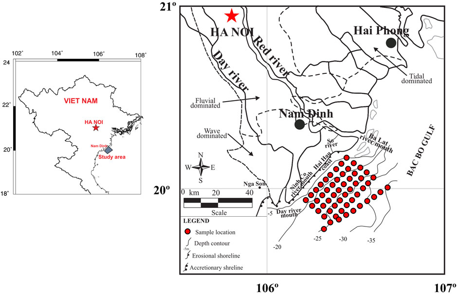
FIGURE 1. Map of the study area and location of surface sediment samples. Area of shoreline erosion and accretion is after Duc et al. (2007). Thin dashed line divides the delta region mostly affected by rivers, tides, and waves, based on the geomorphology (Mather et al., 1996; Mathers and Zalasiewicz, 1999).
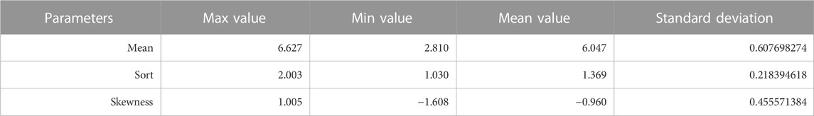
TABLE 1. Input parameter values of the sediment in the study area.
EMMA, which estimates end member scores based on co-variability within grain size distributions, is a powerful tool yielding information on sediment provenance, transport, and depositional environment. EMMA is based on the study of the grain size distribution of sediment samples. It provides a direct link between particle size changes and the physical laws governing sediment production and transport (Weltje and Prins, 2003; Weltje and Prins, 2007). Particle-sized component results from the Horiba LA 960 were used as input values for the EMMAgeo library for processing and performing the grain size distribution (Dietzel E and Dietzel M, 2012, 2019). The calculation steps are provided by Dietzel et al. (2012); Dietzel and Dietzel (2019), including:
Step 1. Transform raw grain size distributions to a constant sum (e.g., 1 or 100%).
Step 2, rescaling and standardization: Minimize the effects of scale by applying a column-wise weight transformation. A weighted matrix W is derived from the columns of the original matrix X by scaling the columns based on percentiles, P, with lower (l) and upper (100−l) boundaries as weights:
where vectors h and g are defined by hj=Pl(xj) and gj=P100−l(xj) for columns j = 1,2,…,p. A value of l = 0 reflects the minimum and maximum of each column; for example, a value of l = 2.5 gives percentiles between P2.5 and P97.5. For the sake of simplicity, we set lw to 0.05; however, note that the optimal value lopt is found by iteration.
Step 3. Calculate eigenvector and eigenvalue matrices. Extract the eigenvector matrix V and eigenvalue matrix Λ from the minor product matrix Γ given by
Step 4, factor rotation: Apply factor rotation (e.g., VARIMAX) on the eigenspace of q end members to simplify the structure of the end members, thus facilitating factor interpretation. The number of end members (q) needs to be determined by iteration.
Step 5. Normalize the preliminary eigenvector loadings (V) to ensure the non-negativity of the rotated eigenvectors and estimate the eigenvector scores (M) using linear non-negative least squares as the objective function. This matrix contains the relative contributions of each end member to each sample. Usually, scores can be interpreted as time series, depth series, or spatial distribution patterns of end member abundance.
Step 6. Rescale matrices and compute variance explained. Reverse the initial weight transformation to rescale V and M to the original units of the initial data set. Normalize the rescaled matrices to fulfill the constant sum constraint. The rescaled and standardized matrices are denoted as end member loadings (V∗) and end member scores (M∗), respectively. Calculate the variance explained by each end member as the proportion of total scores variance. Scores are the relative contributions of the loadings to a sample and are thus related to the predominance of a process during the formation of the sedimentary deposit.
Step 7. Evaluate goodness of model fit. Calculate the modeled data set and the respective error matrix. Evaluate the goodness of fit, calculating mean row- and column-wise linear coefficients of determinations (R2) between X and X∗. The resulting matrix gives the explained proportion of variance of each sample and each variable, respectively (Dietzel et al., 2012).
According to McLaren and Bowles (1985), the direction of net sediment transport from a sediment sample point T1 to another point T2, measured in ɸ, can be either better sorted, finer, and more negatively skewed or better sorted, coarser, and more positively skewed. The vector that indicates the sediment trend is defined by the parameters (Md, So, and Sk) and compared with neighboring samples (stations) through sampling radius (characteristic distance; Dcr). Poizot and Méar, (2010), proposed to define the Dcr parameter (then renamed Dg) after a variogram study process. At a station there may be no or more than one unit trend vectors. In the case of multiple unit trend vectors, a single vector is computed according to Formula 5:
where n is the number of trend vectors identified for the site,
From the geostatistical analysis initially performed to define the characteristic distance Dg, a model of spatial variation is inferred, allowing for interpolations of the three statistical parameters. This operation aims to build regular grids with points equally spaced to allow the same weight for each surrounding neighborhood during vector field computation (Poizot et al., 2006).
Statistically, there are eight total combinations between the parameters Md, So, and Sk. However, Gao and Collins (1992) suggest that the combination of two of them—1) finer, better sorted, and more negative skewness (FB-) and 2) coarser, better sorted, and more positive skewness (CB+)—can be adopted to define the net transport direction. Field observations validate these combinations, as they present the highest probability of occurrence in the net transport direction.
The grain size distribution of surface (0–5 cm) samples (Figure 2) in the study area is wide-ranging, from 0 to 890 μm, and has frequency peaks between 7 and 300 μm. Samples from most locations are mainly composed of fine particle sediments.
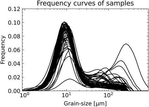
FIGURE 2. Grain size distribution curve of sediment samples in the study area.
Using EMMAgeo, the Rt2 has been calculated from the data set (Figure 3A) using 2 to 10 EM. The results show that with 2 EM, the coefficient reaches 0.77 and that this value increases gradually (0.855, 0.86, 0.89) as the number of end members increases to 3, 4, and 5. Using 4 and 5 EM, most of the grain sizes from the model results are consistent with the dataset. By increasing the number of end members, the average coefficient does not increase and tends to decrease, showing the optimal model results at 5 EM.
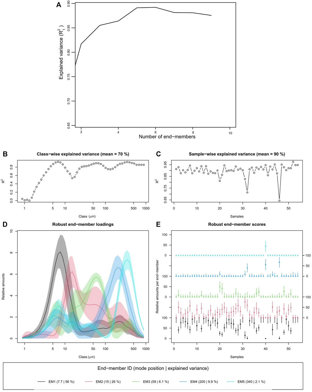
FIGURE 3. End member analysis of surface sediment grain size data from the study area. (A) Coefficient of determination versus the number of end-members; (B,C) explained variance chart for class and sample; (D) location of mode position with explained variance of each EM; (E) end-member score for each EM.
Figure 3 shows the default graphical output, provided by EMMAgeo, for five end members. Panels b and c depict R2 values (squared Pearson correlation coefficients) organized by grain size class and sample of 0.7 and 0.9, respectively. Overall, the data set was reproduced with a mean R2t of 0.89 (Figure 3A). The mode position and explained variance for EM1–EM5 were 56%, 26%, 6.1%, 9.9%, and 2.1%, respectively.
Each end member clearly has a dominant peak and shows a normal distribution in the grain size distribution curves of the five end members (Figure 3D). The grain size of the dominant peak increases, and the sorting improves toward finer grain size at different degrees from EM1 to EM5. EM1 has a mode position of 7.7 μm, with a majority in the fine silt range. EM2 has a mode of 15 μm, with a majority in the medium silt range. EM3 has a mode of 59 μm, with a majority in the very coarse silt range. EM4 has a mode of 200 μm, with a majority in the fine sand range, and EM5 has a mode of 340 μm, with a majority in the medium sand range. EM1 to EM5 have secondary peaks with lower peak values in the fine silt to medium sand range.
Figure 4 shows the spatial distributions of the relative contents of the five end members, which range from 0% to 100%. The content of EM1 was generally higher in the study area (Figure 4A), where the highest values, largely over 70%, are concentrated in the central area (yellow-orange to red zone). The statistics show that samples with content of EM1 > 70% account for 59.2% (32/54 positions), that 12/54 (∼22.2%) positions have a maximum value of 100%, and that only three samples have 0% EM1 content. In general, the large EM1 content (over 70%) has a banded shape, large width, and is oriented parallel to the shore at a water depth of about 15–30 m.
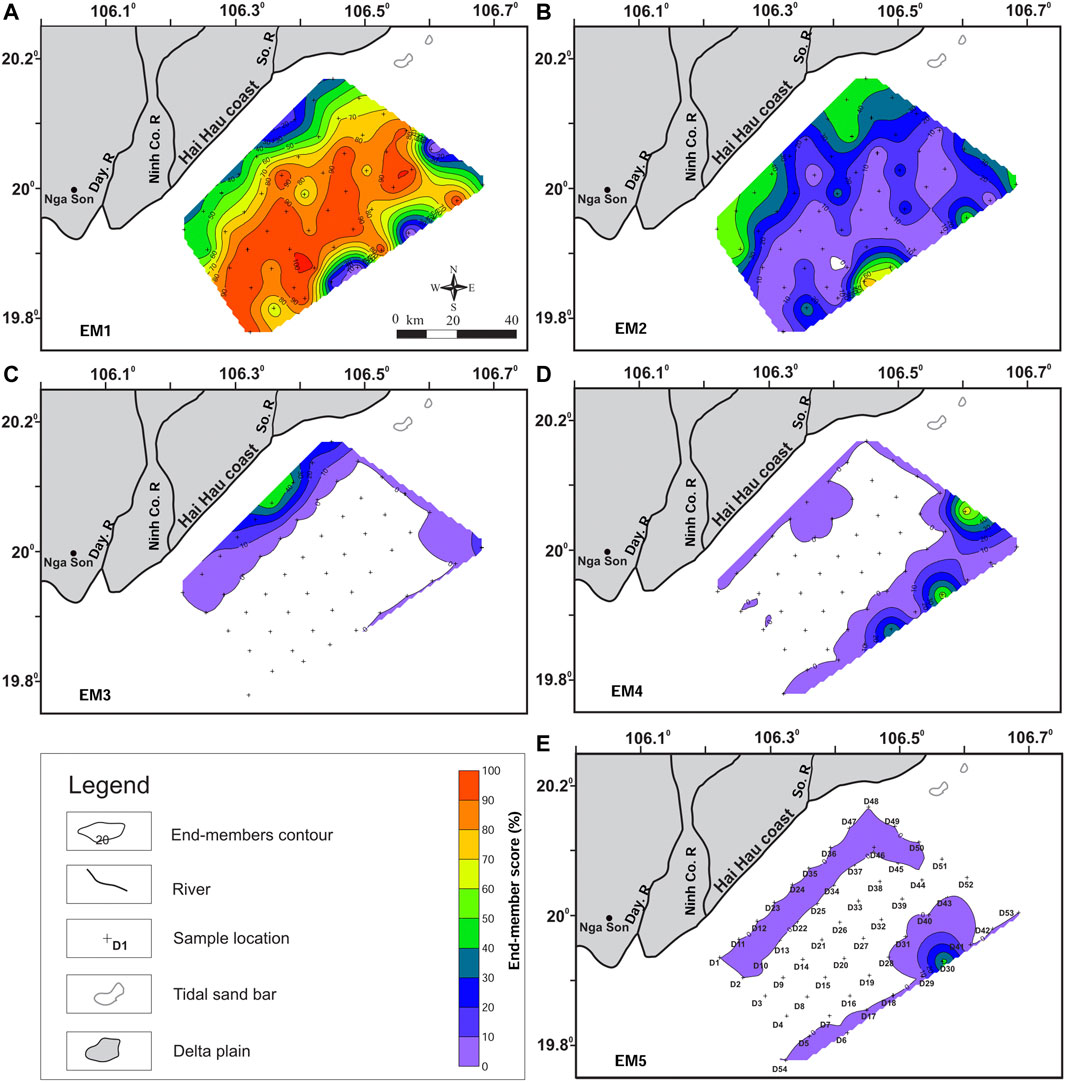
FIGURE 4. Spatial distribution and relative contents of the five end members in the studied area.
In contrast, the EM2 content is relatively low in the central part of the study area (0%–15%), where the majority of EM1 content is concentrated. The EM2 content exceeded 40% in three areas: 1) the southeast of Ninh Co River mouth, 2) the So River mouth with a banded shape oriented parallel to the shore, and 3) the southeast of study area with a higher content and a thicker contour line, where the highest values were recorded. According to statistics, in the study area, EM2 values were not recorded at 14/54 sites (EM2 values equal to 0%); all these are sites with 100% EM1 content, except at positions D29 and D30.
The content of EM3 is relatively low (Figure 4C), with an average value of 22% throughout the study area, locally higher in the coastal area and highest in the So River mouth offshore area, with the highest content values at D35 (48.5%) and D36 (40.7%), with the rest less than 25%.
The EM4 content is similar to EM3 in terms of locality, but it is mainly distributed in the offshore area, stretching from the east to the southeast (Figure 4D). The higher content is concentrated in locations with a higher depth of seabed; the highest value reaches ∼67% at D52, 56% at D30%, and 40% at D18, while the remaining sites have a content of <10%. The EM5 content is concentrated mainly in the D30 sample area with a maximum value of ∼44% (Figure 4E).
Figure 5 and Figure 6 show the relative content of EM1+2+3 and EM4+5, based on the type of sediment (silt sediment and sand sediment, respectively). It can be seen that EM1+2+3 covers almost the entire study area, while EM4+5 is only locally deposited at the outer border of the study area.
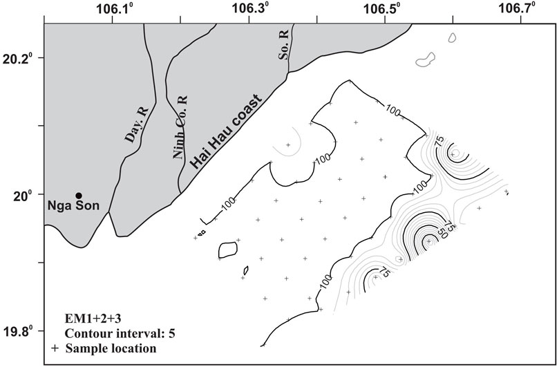
FIGURE 5. Spatial distribution and relative content (contour line) of EM1+2+3 in the study area.
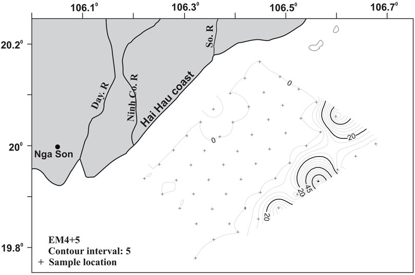
FIGURE 6. Spatial distribution and relative content (contour line) of EM4+5 in the study area.
EM1 and EM2 are quasi-complementary. The highest values of the former are the lowest of the latter, and vice versa. Both EMs gather more than 80% of the EMMA analysis information.
The FB- trend case is clearly correlated with the growing gradient values of EM1. This trend case shows transport from the lower values toward the highest values of EM1. These gradients have the highest values in two areas. The first is inside a strip parallel to the coast and covering 1/3 of the studied area Figure 7, zone A. The second is in the NE-most offshore sector Figure 7, zone B. In the central part of the studied area, corresponding to the highest percentage of EM1 and lowest gradients, FB- trends are rare or even absent. As EM1 corresponds to the finest sediment particle of the study, it can be inferred that the FB- trend case shows the transport of the finest fraction of the sediment. The FB- trend vector field then describes transport directions over the studied area.
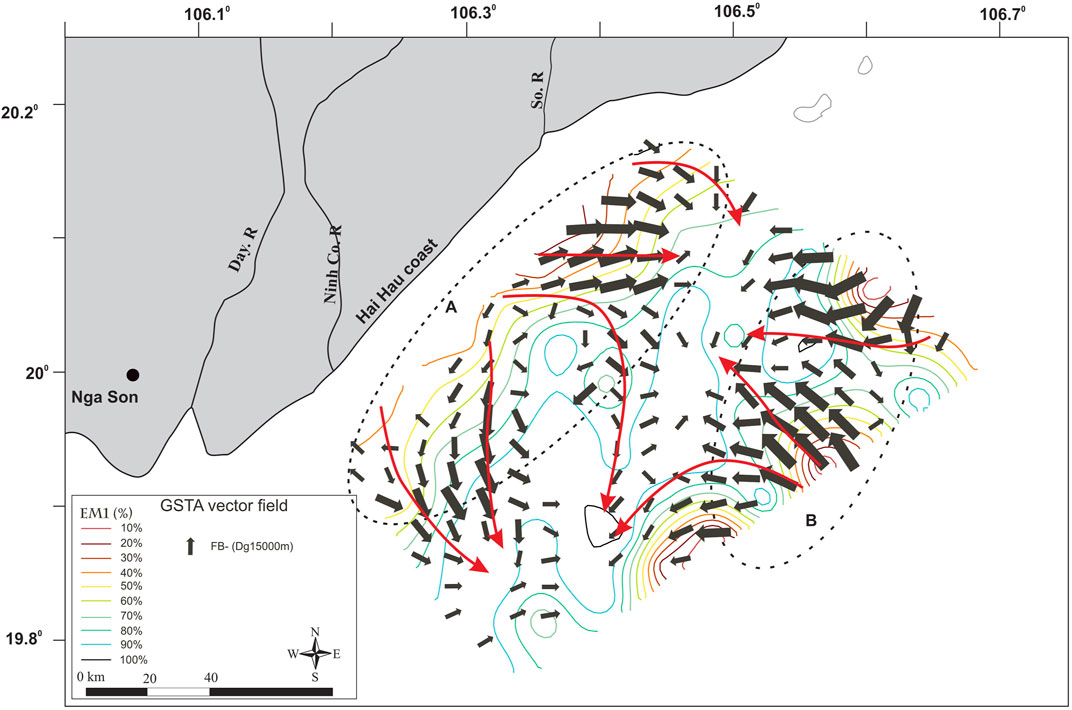
FIGURE 7. Contour lines of EM1 percentage under FB- trend vector field (black arrows) and interpretation (red arrows).
The CB+ trend case shows vectors mainly located over the highest percentage of EM1 (Figure 8). Globally, CB+ vectors are computed over areas where the FB- trend case shows few or even no vectors. Comparisons of the CB+ trend case with the other end members (2–5) do not highlight any particular correlation to the spatial organization. In the context of the current study, the CB+ trend case seems not to represent any kind of transport but more a sediment lag deposit behavior (McLaren, 1981).
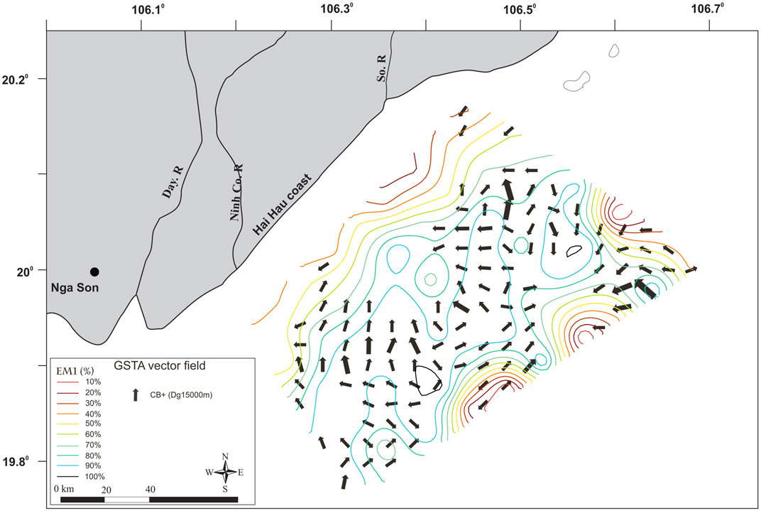
FIGURE 8. Contour lines of EM1 percentage with interpretation of the CB+ vector field.
The combination of FB- and CB+ trends allows the identification of sediment transport vector trends (Figure 9). The patterns show distinct trends in three different zones. In zone 1, with a water depth of 0–15 m, the characteristic sediment transport trend is from the shore to the central area; the part around the So River mouth transports locally towards the northeast, the lower part transports along the coast to the southwest but in small quantity (the length of vector is smaller). Zone 2, at a depth of 25 m upwards, is characteristic of the transport vector from the northeast down and offshore. Transport vectors represented by Gebco bathymetry and the isometric line EM1+2+3 (mud sediment) show that in the region with high content of coarse grain size (specifically sand, where EM4+5 exists), the vectors have a greater module than those in the mud sediment area. In zone 3, the transition between zone 1 and zone 2, at a water depth of about 15–25 m and where mud sediments are dominant, sediment transport trends are unclear.
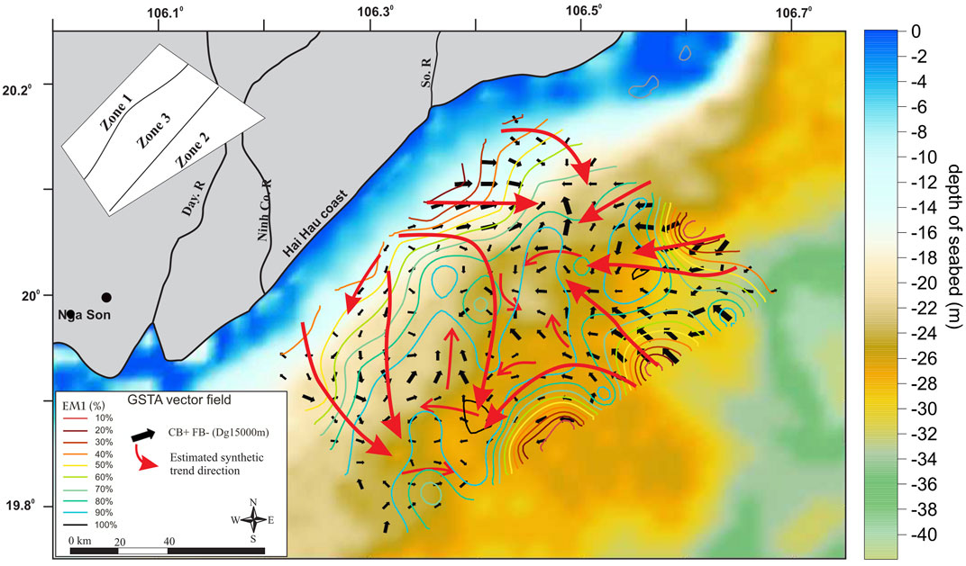
FIGURE 9. Spatial distribution of vectors and trends of general sediment transport, background of Gebco seabed depth, and contour line showing the relative content of EM1(%).
Morphological and depositional characteristics are directly controlled by the complex hydrodynamic regime, which incorporates the regional monsoon, tides, ocean circulation, and coastal currents (Alexander et al., 1991).
The EMMAgeo model results (Figure 4) show that fine and coarse silt sediments (EM1+EM2) mostly occupy the central part of the study area (about <25 m water depth, for 56% and 26%, respectively). The fine-grained fraction (EM1) is mainly in the central part. The coarser-grained part exists on the two offshore sides of the So River mouth. A small amount of very coarse silt (EM3–6.1%) is found in the So River mouth area, while fine to medium sand (EM4, EM5) is mainly concentrated offshore, at water depths of >25 m.
Based on the distribution and orientation of EMs, combined with geomorphological features (Mather et al., 1996; Mathers and Zalasiewicz, 1999), northeast monsoon conditions (Figure 1), and the dominant wave direction from NE–SW (Duong Ngoc Tien, 2012; Huu et al., 2012), it can be hypothesized that EM1 and EM2 are affected by currents and waves along the coast. The source of EM1 (fine silt) may be erosion from the Hai Hau shore or from the north (Ba Lat River mouth area) and transport by irregular dynamic processes (sometimes strong, sometimes static) down to 28 m water depth. Coarser sediment (medium silt corresponding to EM2) is less affected by the river flow into the sea, and it is probably retained on the two banks of the riverbed. Medium silt observed on the offshore side is likely sourced from the coast of Hai Hau (for the nearshore-distributed part) and from the offshore area (for the locally distributed part). The EM3 fraction (very coarse silt) occurs in the outer area of the So River mouth, being transported from the So River. Sediment represented by EM4+5, due to its size and location (below 28 m), is likely deposited under the influence of the most energetic events of annual recurrence. Its source is tentatively assigned to the Ba Lat mouth, and it accumulates in deeper water environments or is transported from neighboring offshore areas under the influence of bottom currents.
Results of predictions of the general sediment trend from GSTA (Figure 9) in relation to the depth background have documented three distinct zones: in zone 1 (0–15 m water depth), sediment is transported from the shore to the offshore area; in zone 2 (>25 m water depth), sediment is transported from the northeast and from the offshore area; and zone 3 (15–25 m water depth) is a mixed zone in which sediment is transported from the north to the southeast and from the two previous zones. Sediments in this latter zone have no apparent clear trend. It is possible that they are subject to the mixed influence of river–sea interactions, where the impact of the sea is greater (Khac Nghia et al., 2013), causing constant disturbance, which gives the sediments collected in the area poor selectivity of 88.9%.
Representation of prediction results of sediment transport trends from GSTA in relation to mud sediments (EM1+2+3) shows that the higher the mud content, the more complex the direction of sediment transport (Figure 9).
The combination of EMMA and GSTA methods leads to the following three observations. First, sediment transport is closely related to fine-grained end members (EM1+2+3). Second, sediments in the Hai Hau–Nam Dinh offshore region are provided by three main sources, including erosion along the Hai Hau coast, sediment from the Ba Lat River mouth, and deep water environments outside the study area. Sediment transport is dominated by the river–sea interaction, which is evident in the center of the study area. Sediment destruction along the Hai Hau coast is due to the erosion mentioned in recent studies and a lack of natural sediment supply due to damming of the So River (Tranet al., 2018). Third, sediments along the Hai Hau coast are eroded and carried to the sea; most of the fine-grained fraction (EM1+2+3) is transported away from the coast and deposited in the center of the study area under the influence of various dynamic processes. The fine-grained component in the center of the study area may also derive from the Ba Lat River mouth; a part of the sand sediment (EM4+5) from the Ba Lat River mouth is also transported down but accumulates in deeper water environments (over 28 m).
Five grain size end members (EM1–EM5) have been identified by the EMMAgeo model. EM1 (fine silt) is possibly originated from sediments eroded in the Hai Hau shore or delivered from the north (Ba Lat River mouth area). The source of EM2 (coarse silt) may be the coast of Hai Hau (for the nearshore-distributed part) and the offshore area (for the locally distributed part). EM3 (very coarse silt) is likely derived from the So River area. EM4+5 (fine-medium sand) is interpreted to have been transported from the Ba Lat River mouth and locally deposited at relatively deep locations.
The combination approach using EMMAgeo and GSTA predicted the transport mechanism of sediments at sampling sites. Sediments in the study area are supplied by three main sources, including erosion along the Hai Hau coast, sediment from the Ba Lat River mouth, and deeper water environments outside the study area. Continuous river–sea interaction is evident in the center of the study area. Sediments along the Hai Hau coast are eroded and carried to the sea; most of the fine-grained sediments (EM1+2+3) are transported away from the shore and deposited in the center of the study area under the influence of various dynamic processes. In addition, the fine-grained components in the center can also derive from the Ba Lat River mouth. A part of the sand sediment (EM4+5) from the Ba Lat River mouth is also transported in deep water areas (below 28 m water depth).
The combination of EMMA and GSTA proved a reliable picture of sediment transport in coastal areas. These two methods are based on same and simple information to get granulometric data. EMMA alone gives footprints of characteristic grain-size distributions, which then help GSTA to better identify the best trend case to compute the transport vector field. Because these two approaches are based on field data sets, the results of their application can be used by hydro-sedimentary numerical models to set and validate sediment transport.
The original contributions presented in the study are included in the article/Supplementary Material, and further inquiries can be directed to the corresponding author.
NV, NH, and TT processed sediment samples, analyzed the grain sizes and the results from the Horiba LA960 device. MD and LA conducted data processing and used and presented EMMA model results. EP, MD, and TT processed, used, and analyzed GSTA model data and outlined the idea of model results. DH and DC reviewed the results of two models and considered the correlation with the collected documents.
The paper is supported by the projects coded UQĐTCB.03/20-21, ĐTĐLCN.59/22-C, and NVCC24.03/22-23.
The authors declare that the research was conducted in the absence of any commercial or financial relationships that could be construed as a potential conflict of interest.
All claims expressed in this article are solely those of the authors and do not necessarily represent those of their affiliated organizations, or those of the publisher, the editors and the reviewers. Any product that may be evaluated in this article, or claim that may be made by its manufacturer, is not guaranteed or endorsed by the publisher.
The Supplementary Material for this article can be found online at: https://www.frontiersin.org/articles/10.3389/feart.2023.1099730/full#supplementary-material
Alexander, C. R., DeMaster, D. J., and Nittrouer, C. A. (1991). Sediment accumulation in a modern epicontinental-shelf setting: The Yellow Sea. Mar. Geol. 98, 51–72. doi:10.1016/0025-3227(91)90035-3
Asselman, N. E. M. (1999). Grain size trends used to assess the effective discharge for floodplain sedimentation, river Waal, The Netherlands. J. Sediment. Res. 69, 51–61. doi:10.2110/jsr.69.51
Blott, S. J., and Pye, K. (2001). Gradistat: A grain size distribution and statistics package for the analysis of unconsolidated sediments. Earth Surf. Process Landf. 26, 1237–1248. doi:10.1002/esp.261
Carriquiry, J., Sánchez, A., and Camacho-Ibar, V. (2001). Sedimentation in the northern Gulf of California after cessation of the Colorado River discharge. Sediment. Geol. 144, 37–62. doi:10.1016/s0037-0738(01)00134-8
Collins, J. D., O’Grady, P., Langford, R. P., and Gill, T. E. (2016). End-member mixing analysis (EMMA) apllied to sediment grainsize distributions to characterize formational processes of the main excavation block, unit 2, of the rimrock draw rockshelter (35ha3855), harney basin, eastern Oregon (USA). Archaeometry 59, 331–345. doi:10.1111/arcm.12243
Dietze, E., and Dietzel, M. (2019). Grain-size distribution unmixing using the R package EMMAgeo. E&G Quat. Sci. J. 68, 29–46. doi:10.5194/egqsj-68-29-2019
Dietze, E., Hartmann, K., Diekmann, B., Ijmker, J., Lehmkuhl, F., Opitz, S., et al. (2012). An end-member algorithm for deciphering modern detrital processes from lake sediments of lake Donggi Cona, NE Tibetan plateau, China. Sediment. Geol. 243-244, 169–180. doi:10.1016/j.sedgeo.2011.09.014
Duc, D. M., Nhuan, M. T., Tran, N., Tien, D. M., van Weering, T. C. E., and van den Bergh, G. D. (2007). Sediment distribution and transport at the nearshore zone of the Red River delta, Northern Vietnam. J. Asian Earth Sci. 29, 558–565. doi:10.1016/j.jseaes.2006.03.007
Duc, D. M., Thanh, D. X., Quynh, D. T., and McLaren, P. (2016). Analysis of sediment distribution and transport for mitigation of sand deposition hazard in Tam Quan estuary, Vietnam. Vietnam. Environ. Earth Sci. 75, 741. doi:10.1007/s12665-016-5560-2
Duc, D. M., Nghi, T., Nhuan, M. T., and Tien, D. M. (2003). Net sediment transport pathways inferred from grain-size analysis. Vietnam J. Geol. 276 5–6. Available at: http://www.idm.gov.vn/Data/TapChi/2003/276/t46.htm. Available at: http://www.idm.gov.vn/Data/TapChi/2003/276/t54.htm.
Duong Ngoc Tien (2012). Analysis of the sediment transport trend and changes of shoreline and bottom of the Day rivermouth using Mike model. Msc thesis of oceanography. Vietnamese: Hanoi University of Science.
Flemming, B. W. (1988). “Process and pattern of sediment mixing in a microtidal coastal lagoon along the west coast of South Africa,” in Tide-influenced sedimentary environments and facies. Editors P. L. de Boer, A. van Gelder, and S. D. Nio (Dordrecht: Reidel), 275–288.
Flemming, B. W. (2007). The influence of grain-size analysis methods and sediment mixing on curve shapes and textural parameters: Implications for sediment trend analysis. Sediment. Geol. 202, 425–435, doi:10.1016/j.sedgeo.2007.03.018
Folk, R. L., and Ward, W. C. (1957). Brazos River bar: a study in the significance of grain size parameters. J. Sediment. Petrol. 27, 3–26.
Gao, S., Collins, M. B., Lanckneus, J., Moor, G. D., and Lancker, V. V. (1994). Grain size trends associated with net sediment transport patterns: An example from the Belgian continental shelf. Mar. Geol. 121, 171–185. doi:10.1016/0025-3227(94)90029-9
Gao, S., and Collins, M. (1992). Net sediment transport patterns inferred from grain-size trends, based upon definition of ‘‘transport vectors. Sediment. Geol. 80, 47–60.
Hoan, L. X., Hanson, H., Larson, M., Donnelly, C., and Nam, P. T. (2009). Modeling shoreline evolution at Hai Hau beach, Vietnam. J. Coast. Res. 25 (0), 000. doi:10.2112/08-1061.1
Huang, H. Q. (2010). Reformulation of the bed load equation of Meyer-Peter and Müller in light of the linearity theory for alluvial channel flow. Water Resour. Res. 46, W09533. doi:10.1029/2009WR008974
Hughes, S. A. (2005). Use of sediment trend analysis (STA) for coastal projects ERDC/CHL chetn-VI-40. Vicksburg, MS: US Army Corps of Engineers, 17.
Huu, V. C., Hoan, L. X., and Son, N. M. (2012). Calculation of waves and sediment transport in the nearshore Hai Hau - Nam Dinh. J. Water Resour. Sci. Technol. 2012, 7. Available at: https://www.vawr.org.vn/tinh-toan-song-va-van-chuyen-bun-cat-tai-vung-bien-ven-bo-hai-hau-nam-dinh.
Jia, J., Gao, S., and Xue, Y. (2003). Sediment dynamic processes of the Yuehu inlet system, Shandong peninsula, China. Estuar. Coast Shelf Sci. 57, 783–801. doi:10.1016/s0272-7714(02)00406-7
Khac Nghia, N., Dan, M. A., and Tuan, N. A. (2013). Evolution of Lach Giang estuary through analysis of historical documents, satellite images and political orientation to stabilize the coast. J. Water Resour. Sci. Technol. 2013, 16. Available at: https://www.vawr.org.vn/images/File/PGS.TS.%20Nguyen%20Khac%20Nghia.pdf.
Le Roux, J. P. (1994). Net sediment transport patterns inferred from grain-size trends, based upon definition of “transport vectors” - comment. Sediment. Geol. 90, 153–156. doi:10.1016/0037-0738(94)90022-1
Le Roux, J., and Rojas, E. (2007). Sediment transport patterns determined from grain size parameters: Overview and state of the art. Sediment. Geol. 202, 473–488. doi:10.1016/j.sedgeo.2007.03.014
Li, T., and Li, T. J. (2018). Sediment transport processes in the Pearl River Estuary as revealed by grain-size end-member modeling and sediment trend analysis. Geo-Mar Lett. 38, 167–178. doi:10.1007/s00367-017-0518-2
López-González, N., Alonso, B., Juan, C., Ercilla, G., Bozzano, G., Cacho, I., et al. (2019). 133,000 Years of sedimentary record in a contourite drift in the western alboran sea: Sediment sources and paleocurrent reconstruction. Geosciences 9 (8), 345. doi:10.3390/geosciences9080345
Masselink, G. (1992). Longshore variation of grain size distributions along the coast of the Rhone Delta, South. France a test “Mc Laren Model.” J. Coast. Res. 8, 286–291.
Mather, S. J., Davies, J., Mc Donal, A., Zalasiewicz, J. A., and Marsh, S. (1996). The red River Delta of Vietnam. British Geological Survey Tecchnical Report WC/96/02, 41p.
Mathers, S., and Zalasiewicz, J. (1999). Holocene sedimentary architecture of the red River delta, Vietnam. J. Coast. Res. 15, 314–325.
McLaren, P., and Beveridge, P. (2006). Sediment trend analysis of the hylebos waterway: Implications for liability allocations. Integr. Environ. Assess. Manag. 2 (3), 262–272. doi:10.1002/ieam.5630020306
McLaren, P., and Bowles, D. (1985). The effects of sediment transport on grain-size distributions. J. Sediment Pet. 4:457–470.
McLaren, P., Hill, S. H., and Bowles, D. (2007). Deriving transport pathways in a sediment trend analysis (STA). Sediment. Geol. 202, 489–498. doi:10.1016/j.sedgeo.2007.03.011
McLaren, P. (1981). An interpretation of trends in grain size measures. J. Sediment. Pet. 51, 611–624.
Nghi, T., Nhan, T. T. T., Dien, T. N., Thanh, D. X., Dung, T. T., Thao, N. T. P., Truong, T. X., Tuan, D. M., and Lam, D. D. (2018). The Holocene – present shorelinemigration off Thai binh – NamDinh in relation to evolution of deltaic lobes and history of the So River. VNU J. Sci. Earth Environ. Sci. 34 (4), 2588–1094. Available at: https://js.vnu.edu.vn/EES/article/view/4346.
O’Shea, M., and Murphy, J. (2016). The validation of a new GSTA case in a dynamic coastal environment using morphodynamic modelling and bathymetric monitoring. J. Mar. Sci. Eng. 4, 27. doi:10.3390/jmse4010027
Ostrowski, R., Pruszak, Z., Różyński, G., Szmytkiewicz, M., and Van Ninh, P. (2009). Coastal processes at selected shore segments of south BalticSea and gulf of tonkin (south China sea). Archives Hydro-Engineering Environ. Mech. 56 (1–2), 3–28. Available at: http://www.ibwpan.gda.pl/storage/app/media/ahem/ahem56str003.pdf.
Paladino, Í. M., Mengatto, M. F., Mahiques, M. M., Noernberg, M. A., and Nagai, R. H. (2022). End-member modeling and sediment trend analysis as tools for sedimentary processes inference in a subtropical estuary. Estuar. Coast. Shelf Sci. 278, 108126. doi:10.1016/j.ecss.2022.108126
Paterson, G. A., and Heslop, D. (2015). New methods for unmixing sediment grain size data. Geochem. Geophys. Geosyst. 16, 4494–4506. doi:10.1002/2015GC006070
Pedreros, R., Howa, H. L., and Michel, D. (1996). Application of grain size trend analysis for the determination of sediment transport pathways in intertidal areas. Mar. Geol. 135, 35–49. doi:10.1016/s0025-3227(96)00042-4
Poizot, E., Méar, Y., and Biscara, L. (2008). Sediment trend analysis through the variation of granulometric parameters: A review of theories and applications. Earth Sci. Rev. 86, 15–41. doi:10.1016/j.earscirev.2007.07.004
Poizot, E., Mear, Y., Thomas, M., and Garnaud, S. (2006). The application of geostatistics in defining the characteristic distance for grain size trend analysis. Comput. Geosci. 32, 360–370. doi:10.1016/j.cageo.2005.06.023
Poizot, E., and Méar, Y. (2010). Using a GIS to enhance grain size trend analysis. Environ. Model. Softw. 25, 513–525. doi:10.1016/j.envsoft.2009.10.002
Prins, M. A., Bouwer, L. M., Beets, C. J., Troelstra, S. R., Weltje, G. J., Kruk, R. W., et al. (2002). ocean circulation and iceberg discharge in the glacial north atlantic: Inferences from unmixing of sediment size distributions. Geology 30, 555–558. doi:10.1130/0091-7613(2002)030<0555:ocaidi>2.0.co;2
Pruszak, Z., Szmytkiewicz, M., NguyenHung, M., and Pham Van Ninh, (2002). Coastal processes in the red river delta area, Viet Nam. Coast. Eng. J. 44 (2), 97–126. doi:10.1142/s0578563402000469
Ríos, F., Cisternas, M., Le Roux, J., and Corréa, I. (2002). Seasonal sediment transport pathways in Lirquen Harbor, Chile, as inferred from grain-size trends. Investe. Mar. Valpso. 30 (1), 3–23. doi:10.4067/s0717-71782002000100001
Shore Protection Manual (1984). Coastal engineering research center. Vicksburg, Mississippi: US Army Corps of Engineers.
van Lancker, V., Lanckneus, J., Hearn, S., Hoekstra, P., Levoy, F., Miles, J., et al. (2004). Coastal and nearshore morphology, bedforms and sediment transport pathways at Teignmouth (UK). Cont. Shelf Res. 24, 1171–1202. doi:10.1016/j.csr.2004.03.003
Weltje, G. J., and Prins, M. A. (2007). Genetically meaningful decomposition of grain-size distributions. Sed. Geol. 202, 409–424. doi:10.1016/j.sedgeo.2007.03.007
Weltje, G. J., and Prins, M. A. (2003). Muddled or mixed? Inferring palaeoclimate from size distributions of deep-sea clastics. Sediment. Geol. 162, 39–62. doi:10.1016/s0037-0738(03)00235-5
Keywords: sediment trend, Red River Delta, end member modeling analysis, grain size trend analysis, Hai Hau coast
Citation: Dong MD, Poizot E, Cuong DH, Anh LD, Hung DQ, Thuy Huong TT, Diep NV and Huong NB (2023) Transport trend of recent sediment within the nearshore seabed of Hai Hau, Nam Dinh province, southwest Red River Delta. Front. Earth Sci. 11:1099730. doi: 10.3389/feart.2023.1099730
Received: 16 November 2022; Accepted: 27 February 2023;
Published: 17 March 2023.
Edited by:
Alessandro Amorosi, University of Bologna, ItalyCopyright © 2023 Dong, Poizot, Cuong, Anh, Hung, Thuy Huong, Diep and Huong. This is an open-access article distributed under the terms of the Creative Commons Attribution License (CC BY). The use, distribution or reproduction in other forums is permitted, provided the original author(s) and the copyright owner(s) are credited and that the original publication in this journal is cited, in accordance with accepted academic practice. No use, distribution or reproduction is permitted which does not comply with these terms.
*Correspondence: Mai Duc Dong, ZHVjZG9uZy5nZW9AZ21haWwuY29t
Disclaimer: All claims expressed in this article are solely those of the authors and do not necessarily represent those of their affiliated organizations, or those of the publisher, the editors and the reviewers. Any product that may be evaluated in this article or claim that may be made by its manufacturer is not guaranteed or endorsed by the publisher.
Research integrity at Frontiers
Learn more about the work of our research integrity team to safeguard the quality of each article we publish.