 Deqiang Zhang
 Chongguang Pang1,3,4*
94% of researchers rate our articles as excellent or good
Learn more about the work of our research integrity team to safeguard the quality of each article we publish.
Find out more
ORIGINAL RESEARCH article
Front. Earth Sci., 10 May 2023
Sec. Sedimentology, Stratigraphy and Diagenesis
Volume 11 - 2023 | https://doi.org/10.3389/feart.2023.1097033
This article is part of the Research TopicCohesive Sedimentary Systems: Dynamics and Deposits - Volume IIView all 4 articles
Sedimentary processes in marginal seas play an important role in the biology, physics, and geochemistry as well as ecology of coastal environments and contain abundant information about the material transfer from land to ocean and the regional circulation. Due to the huge sediment discharge of the Yellow River, the Bohai Sea, China is one of the areas with the highest suspended sediment concentration (SSC) in the world. Interestingly, the SSC at the west of the Bohai Sea is low all year round. Thus, it is of great significance to examine the sedimentary dynamic process in this area for better understanding the circulation structure, material exchange and regional environment of the Bohai Sea. Using seabed base observation platform measurements obtained in February 2017 and August 2019, this study examines the winter and summer hydrography and suspended sediment concentration in the sea area off Qinhuangdao located to the west of the Bohai Sea. In summer, the relatively weak residual currents flowed northeastward and showed little correlation with the wind field, especially in the middle layer of the water column. In winter, the residual currents were strengthened, flowing to the northeast during strong wind periods, and predominantly to the southwest during intermittent periods. Moreover, driven by the pressure gradient force associated with the wind-induced sea surface height variations, the winter current was closely related to the wind speed, with correlation coefficients ranging from 0.4 to 0.6 and a time lag of 10 h. The summer SSC was lower and mainly controlled by the tidal current, whereas in winter, owing to the enhanced Reynolds stress and turbulent kinetic energy, strong wind bursts triggered significant sediment resuspension and led to a higher SSC. For the suspended sediment flux (SSF), the advection terms contributed more than 80% in the winter and summer, while the vertical circulation terms contributed 13% in winter, and approximately half that much in summer. Generally, the suspended sediment is transported back and forth, with a little net northward and northeastward motions in winter and summer, respectively. This may explain the low SSC sustaining in coastal Qinhuangdao all year round. These results provide a reference for sedimentary studies conducted in other coastal waters, especially in monsoon-dominating shelf seas.
Suspended sediment plays an important role in the biology, physics, and geochemistry of coastal environments. For example, suspended sediment can have an effect on primary productivity by affecting the extent to which light penetrates the water bodies (Lee et al., 2009; Shi et al., 2017). Suspended sediments can affect the morphodynamic evolution of estuaries and inshore areas through the processes of deposition, flocculation, and settling (Dyer et al., 2000; Wang et al., 2010; Elias et al., 2012). The formation and transportation of suspended sediment plays an important role in the ecological environment of marginal seas (Birch et al., 1999), so exploring the spatial and temporal dynamic processes of suspended sediment concentration (SSC) is of great significance for better understanding the coastal environments.
Due to seasonal changes in ocean dynamics and sediment discharge by rivers, the concentration and transport of suspended sediment in shelf seas exhibit strong seasonal variation (Muslim and Jones, 2003; Yuan et al., 2008; Zhao et al., 2022). The ocean color imageries showed that the SSC in global waters has seasonal variation as well (Wei et al., 2021). Based on the MODIS data from 2003 to 2018, the spatio-temporal variation of SSC in the East China Sea was studied by Qiao et al. (2020), and it was found that the SSC had a typical seasonal variation. The SSC in the Mekong Delta in southwest Vietnam also has seasonal variation, and due to the decrease of the runoff and sediment discharge, the SSC in coastal waters of the delta shows a decreasing trend (Loisel et al., 2014). As the river with the second largest sediment discharge in the world, the Yellow River flows to the Bohai Sea, making the Bohai Sea one of the seas with the highest SSC in the world (Yang et al., 2011). Therefore, conducting winter and summer observations in the Bohai Sea is crucial for understanding the transport process of coastal sediments and explaining changes in marine environment and ecosystem.
The Bohai Sea located in the north part of East China Seas (Figure 1A), is a semi-enclosed marginal sea consisting of four parts: the Bohai Bay, Liaodong Bay, Laizhou Bay, and Central Basin (Figure 1B). Owing to the Huanghe, Liaohe, Haihe, and Luanhe Rivers carrying large amounts of sediment into the Bohai Sea and the seawater having a poor exchange capacity, the suspended sediment concentration (SSC) in the Bohai Sea is higher than that in other East China seas (Bian et al., 2013; Wang et al., 2016). Consequently, in recent decades, the high SSC in the Bohai Sea has been widely studied, especially Mao et al. (2018) and Zhao et al. (2022) considered the entire Bohai Sea. Since the majority of previous studies have concentrated on the resuspension, transportation and final destination of Huanghe River-derived sediment and its seasonal variability, most researchers have focused on specific areas such as the Huanghe Estuary (Li et al., 2010; Qiao et al., 2010; Yang et al., 2011; Wang et al., 2014; Liu et al., 2020a), the Bohai Strait (Duan et al., 2020b; Liu et al., 2020b; Wang et al., 2020), and the Bohai Bay (Qiao et al., 2011), and paid minimal academic attention to other sea areas, such as the exceptional low SSC area off Qinhuangdao (Figure 1B).
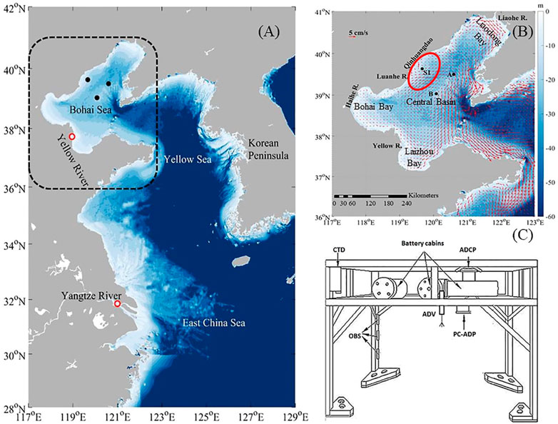
FIGURE 1. (A) Bottom topography of the Bohai Sea, Yellow Sea and East China Sea. (B) Bathymetry of the Bohai Sea (color shading) with the climatological winter depth-averaged current field (arrows). The black dot represents the S1 mooring; the block dots (A,B) represent the locations of the winter and summer wind speed observation buoys; the red circle indicates the exceptionally low SSC area off Qinhuangdao. The velocity data were derived from Liu et al. (2021). (C) Schematic of the seabed base observation platform.
The year-round low SSC and high salinity that dominates the sea area off Qinhuangdao has been mentioned in several studies based on numerical simulation results and remote sensing data, but in situ observations of this area are scarce. Jiang et al. (2004), Wang and Li (2009), Chen et al. (2010), and Bian et al. (2013) conducted numerical simulations of suspended sediments in the Bohai Sea and found a low SSC in the sea area off Qinhuangdao. Wang and Jiang (2008), Cui et al. (2009), Pang and Yu (2013), and Zhao et al. (2022) found that the coastal waters off Qinhuangdao showed the smallest seasonal differences in SSC among those of all Bohai Sea regions, by using ocean color remote sensing data. While the spatial distribution of suspended sediments in the Bohai Sea has been presented in these studies, in-depth research on the underlying dynamic mechanism has yet to be reported, due to the lack of in situ observations.
The vertical distribution of the SSC and its temporal variation are crucial to the dynamical mechanism. Jiang et al. (2020) conducted field observations in the sea area off Qinhuangdao for more than 20 days from February to March 2017, using a bottom-mounted quadropod to obtain the hydrological and sediment parameters at quasi-full water depths, and explored the mechanism of sediment resuspension during a strong wind event in winter. Their research led to the conclusion that, even under the influence of storm winds in the winter, the local weak sediment resuspension causes the formation of the low SSC area off Qinhuangdao.
In East China seas, especially the Bohai Sea, seasonal variations in the SSC is significant since winter and summer monsoons prevail. Yang et al. (2011) studied the seasonal comparison of sediment transport off the Huanghe delta based on observation data and pointed out that the coastal area off the Huanghe delta acts as a sediment sink in summer and converted to be a sediment source in winter in response to the seasonal variation of the East Asian monsoon in this region. Wang et al. (2014) further concluded that strong seasonal variability of suspended sediment distribution in the Bohai Sea was consistent with the monsoon activity and associated wave actions and coastal currents that are varying seasonally. In consideration of strong wind waves causing the seabed sediments to be resuspended and dominating the seasonal variation of the SSC in the Bohai Sea, winter monsoon, especially winter storm and its controlling mechanism have been extensively studied (Wu et al., 2019; Duan et al., 2020b; Wang et al., 2020). However, summer observations and studies are relatively rare. Both winter observations and summer field surveys are necessary to depict the complete dynamic sedimentary processes at the study site.
In this study, a seabed base observation platform was deployed to measure the temperature, salinity, echo intensity, current velocity, and so on in the sea area off Qinhuangdao from 15 August to 29 August 2019. The in-situ observational data from the Bohai Sea near Qinhuangdao in the summer of 2019 and winter of 2017 were compared to explore the seasonal differences in SSC and its dynamical mechanism.
Seabed base observation campaigns were conducted in the Bohai Sea off Qinhuangdao from 15 February to 9 March 2017, and from 15 August to 29 August 2019. The sea area off Qinhuangdao is located in the west coast of the Bohai Sea, with the range of 39.45°N—40.70°N and 119.2°E−120.8°E, and it is a key sea area connecting the Liaodong Bay and the Bohai Bay (Figure 1B). The seabed base observation platform placed at Station S1 both in winter and summer, located at 39°38′N and 119°40′E, was 2.2 m × 2 m × 2 m (length × width × height) in size (Figure 1C), with a suite of instruments installed onboard, including an upward-looking Acoustic Doppler Current Profiler (ADCP), a downward-looking Pulse-Coherent Acoustic Doppler Profiler (PC-ADP), an Acoustic Doppler Velocimeter (ADV), three Optical Backscatter Sensors (OBS), and a Conductivity-Temperature-Depth (CTD).
The two seabed base observation campaigns relied on the same quadropod and instruments. Jiang et al. (2020) provided a detailed description of the instruments deployed at Station S1 in the seabed base observation campaign of 2017. Station S1 information from 2017 to 2019, such as longitude and latitude, water depth, instrument configuration and effective observation period, is shown in Table 1. During the 2019 observations, the upward-looking ADCP contained 19 depth units of 1 m each, with the first unit 3.23 m above the transducer. The observed data, such as the velocity and echo intensity in the upper layer, were obtained from ADCP with a time resolution of 30 min with a valid data range of 5.23–16.23 m from the seabed. The downward-looking PC-ADP was placed 1.25 m from the bottom, with a blind area range of 0.05 m. The velocity and echo intensity of the bottom boundary layer were obtained from the PC-ADP with a time resolution of 30 min and valid data range of 0.045–1.100 m from the bottom. Through ADCP and PC-ADP observations, the velocity and echo intensity of the entire water depth were measured. Additionally, the ADV conducted intermittent sampling at a frequency of 16 Hz for 30 s every 30 min to obtain near bottom high-frequency velocity data. Meanwhile, the three OBSs were placed at different heights on the quadropod and used to collect the turbidity of the bottom boundary layer with a sampling interval of 10 min. Owing to the severe oceanic conditions and aging of the instruments, the OBSs were not working properly. The temperature and salinity near the bottom layer were obtained using the CTD with a time resolution of 10 min.
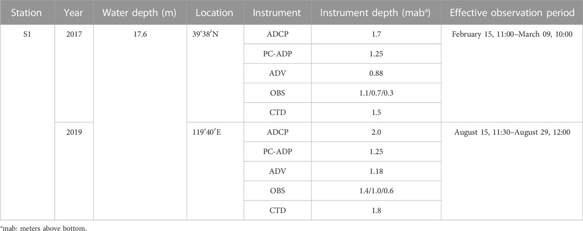
TABLE 1. Comparison of instrument configurations at S1 in the winter of 2017 and summer of 2019.
The SSC was estimated from the correlation between the winter SSC measurements from 2017 and the backscatter intensity. Jiang et al. (2020) used a 1 L water bottle to collect a total of nine water samples from the upper, middle, and lower layers of S1 every 3 h to measure the SSC.
In the winter of 2017, wind speed data were obtained from an offshore buoy located at 39°30′N 120°36′E, as shown at A in Figure 1B. In the summer of 2019, wind speed data were also derived from an offshore buoy, located at 39°02′N 120°05′E (B in Figure 1B).
The Reynolds method was used to calculate the bottom shear stress (
where
The estimation of Reynolds’ stress is done as follows (Li et al., 2018):
The turbulent kinetic energy (TKE) is computed as follows:
where
To obtain the turbulent component, the bandpass filtering method was used to decompose the fluctuating components (Soulsby and Humphery, 1990; Kularatne and Pattiaratchi, 2008; Meirelles et al., 2015; Zhu et al., 2016). By analyzing the power spectrum density of the fluctuating component in the summer of 2019, it was found that the wave periodic signal was not significant, which may be because the wind speed in summer is too small to affect the seabed, so it is not necessary to separate the waves and turbulence. During the winter observation in 2017, the wave frequency was 0.15 hz through power spectrum density analysis, so the turbulent velocity was obtained through a high-pass filter with a cutoff frequency of 0.2 Hz and a low-pass filter with a cutoff frequency of 3.0 Hz.
The wind stress is calculated as follows:
where
The pressure gradient force is calculated as follows:
where
The suspended sediment flux (SSF) is the amount of suspended sediment passing through a specific area (usually a unit area perpendicular to the direction of flow) in a unit time. The average SSF over a tidal cycle can be quantified as follows (Dyer, 1997; Yu et al., 2012; Yu et al., 2014; Pang et al., 2020):
where
Each decomposition term (F1–F7) represents a specific physical process contributing to the SSF (Dyer, 1997; Li and Zhang, 1998; Yu et al., 2012; Pang et al., 2020). The first term (F1) is the non-tidal drift, called the Eulerian flux, and depends on the tidal current intensity comparison, representing the dominant current contribution to the net sediment transport. The second term (F2) is the Stokes drift effect contribution to the net sediment transport. The terms F1 and F2 are related to advection transport and can be combined to form the advection transport terms (known as the Lagrangian flux). The terms F3 to F5 constitute the tidal pumping terms, which are caused by the phase difference between the depth-averaged SSC, the depth-averaged velocity, and the tidal elevation. The terms F6 and F7 result from the vertical circulation effects, and represent the tidally-averaged vertical circulation and the variation in the vertical distribution of the SSC and velocity, respectively.
This decomposition method has been widely used to study sediment flux patterns and maximum turbidity formations in estuaries (de Nijs et al., 2009; Erikson et al., 2013; Ganju et al., 2005; Li and Zhang, 1998; Nowacki et al., 2015; Su and Wang, 1986; Uncles et al., 1985a; Uncles et al., 1985b; Wu et al., 2001; Xiao et al., 2018). Here, the relative importance of different processes are assessed by comparing the values of the decomposition terms.
Figure 2A shows the time series of hourly-averaged wind speeds from 15 February 2017, to 9 March 2017, exhibiting an average value of 6.5 ± 4.0 m/s and a range of 0.3–17.9 m/s; wind speeds greater than 14 m/s were defined as strong wind events (Jiang et al., 2020), with the four strong wind events corresponded to a northerly wind direction. Figure 2C shows the wind speed variations with an hourly mean of 4.5 ± 2.1 m/s and a range of 0.1–11.7 m/s during the observation period from 15 August 2019, to 29 August 2019, with a predominately southerly wind direction. It is clear that the winter wind speed in the sea area off Qinhuangdao is greater than it is in the summer.
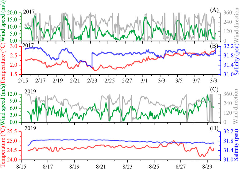
FIGURE 2. Time series of hourly mean wind speed and wind direction: (A) from 10:00 on 15 February 2017 to 10:00 on 9 March 2017; (C) from 11:00 on 15 August 2019 to 12:00 on 29 August 2019. (B) Time series of temperature and salinity with a temporal resolution of 5 min from 10:10 on 15 February 2017 to 10:00 on 10 March 2017. (D) Time series of temperature and salinity with a temporal resolution of 10 min from 11:30 on 15 August 2019 to 12:00 on 29 August 2019.
The sequences of the temperature and salinity near the bottom layer (about 1.5 m above the seabed) from 15 February 2017, to 9 March 2017, are shown in Figure 2B. The salinity and temperature ranged from 31.28 to 32.17 psu and 1.71°C–2.77°C, with mean values of 31.88 ± 0.16 psu and 2.22°C ± 0.29°C, respectively. After each strong wind event, there was a tendency for the salinity near the bottom to decrease, possibly owing to the low salinity seawater input along the coast. The temperature and salinity time series during the August 2019 observation period are shown in Figure 2D. The temperature near the bottom (about 1.8 m above the seabed) spanned a range of 24.16°C–25.02°C with an average value of 24.64°C ± 0.14°C. After 5:00 on 27 August, there was a slight drop in temperature, which may be related to a shift in wind direction from southerly to northerly. Then at 4:00 on 28 August, the temperature dropped further, which may be due to wind speed enhancements. The salinity values (about 1.8 m above the seabed) during the August 2019 observation period were 31.79 ± 0.05 psu, with a range of 31.67–31.86 psu. The winter temperature and salinity variations were larger than those of the summer during the observation periods, which may be a result of the stronger winds transporting the relatively high-temperature, high-salinity water body from the Bohai Strait to S1 in winter.
As shown in Figure 3, regardless of the season, the current at S1 is dominated by irregular semi-diurnal tides, and the current velocity in the middle and upper layer is larger than that in the bottom layer. During the winter 2017 observation period, the maximum and minimum current velocities of the middle and upper layers (measured by ADCP) were 0.73 m/s and 0.10 m/s, respectively, with an average value of 0.20 m/s (Figures 3C, D). The current velocity in the bottom boundary (measured by PC-ADP) ranged from 0 to 0.36 m/s, with an average value of 0.08 m/s (Figures 3B, F). Similarly, the average current velocity (as measured by ADCP) was 0.20 m/s during the summer 2019 observation period, varying from 0.14 to 0.56 m/s (Figures 3C, G). The current velocity in the bottom boundary layer (measured by PC-ADP) varied from 0.07 to 0.28 m/s, with an average value of 0.09 m/s (Figures 3D, H).
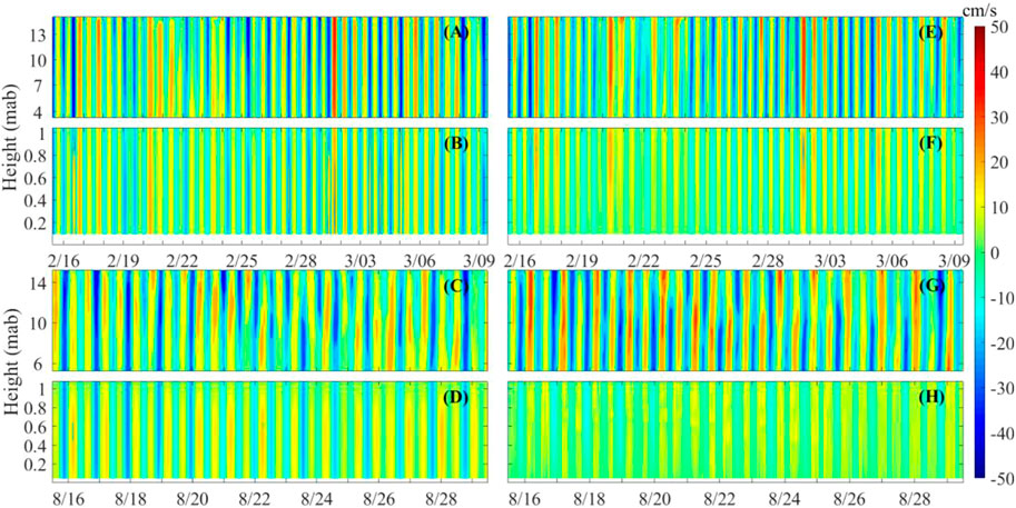
FIGURE 3. Vertical and temporal variability in the current velocity (V component and U component) at S1 collected by the upward-looking ADCP (A,C,E,G) and downward-looking PC-ADP (B,D,F,H), respectively: (A,B,E,F) from 10:00 on 15 February 2017 to 10:20 on 9 March 2017; (C,D,G,H) from 11:30 on 15 August 2019 to 12:00 on 29 August 2019.
The vertical distribution of residual currents time series during the 2017 and 2019 observation periods are shown in Figure 4. The residual currents time series were obtained through a 40 h lowpass filter of the original velocity data to remove the tidal signals.
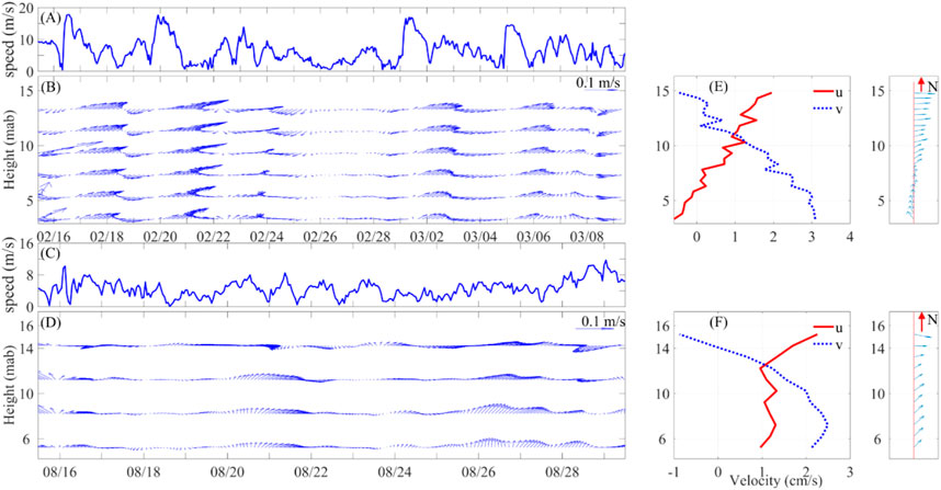
FIGURE 4. Wind speed (A,C), Low-pass filtered (B,D) and temporal averaged (E,F) residual currents observed by the upward-looking ADCP during the winter of 2017 (A,B,E) and summer of 2019 (C,D,F).
Regardless of the observation period, the middle- and upper-layers residual currents were significantly larger than those of the bottom layer, as shown in Figure 4. During the 2017 observation period, the average residual currents of the middle-upper layers and the bottom layers were 5.7 and 3.9 cm/s, respectively (Figure 4B). Residual currents flowed to the northeast during strong wind periods and flowed predominately to the southwest during intermittent periods in the winter of 2017 (Figures 4A, B). Generally, the lower-layer residual current flowed northward while the upper- and middle-layer currents flowed eastward (Figure 4E). However, during the 2019 observation period, the average residual currents of the middle-upper layers and the bottom layer were 3.8 and 1.1 cm/s, respectively (Figure 4D). Generally without the influence of strong wind (Figure 4C), the residual current flowed northeastward.
Jiang et al. (2020) proposed that in the upper and middle water body, the occurrence of high SSC lagged behind the high wind speed by about 10 h. Similarly, approximately 10 h after the onset of a strong wind event, a significant increase in residual current was observed during the 2017 observation period, as shown in Figures 4A, B. The advance and lag correlations between residual currents and wind speeds further indicated that the best correlation was with a 10 h lag. Figure 5 shows the correlations between the wind speeds and residual currents, and the wind speeds and the 10 h lag residual current during the 2017 and 2019 observation periods, respectively. Figures 5A, B show that, during the 2017 observation period, the correlations between the wind speed and residual current were significantly smaller than those between the wind speed and the 10 h lag residual current. This difference was especially noticeable in the layers measured by ADCP. As shown in Figure 5A, the correlations between the wind speed and the residual current were less than 0.1 while those between the wind speed and the 10 h lag residual current were roughly 0.4–0.6.
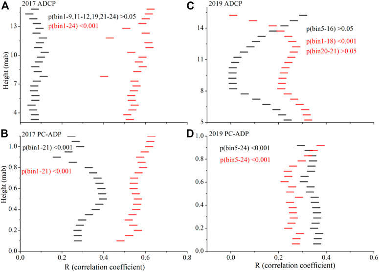
FIGURE 5. Correlations between the wind speed and residual current observed by ADCP (A,C) and PC-ADP (B,D) during the winter of 2017 (A,B) and summer of 2019 (C,D). The short black lines represent the zero-lag correlations and the short red lines represent the correlations when the residual current lags by 10 h.
Figures 5C, D show that, during the 2019 observation period, at the surface layers the correlations between the wind speed and residual current were greater than those between the wind speed and 10 h lag residual current. At the middle layers, the opposite correlations were greater, and two kinds of correlations were similar at the lower and bottom layers. The correlations in the summer were different from those in the winter, which may imply two distinct driving mechanisms. The vertical distribution of correlations displayed that only the surface and bottom friction layers were under the instant influence of summer wind forces; however, summer wind forces were weak, indicating that thermohaline circulation played an important role in the summer residual current (Huang et al., 1999; Liu et al., 2003; Wu et al., 2004; Duan et al., 2020a).
Figures 6, 7 show the winter and summer SSC profiles at full water depth at S1, where ADCP measured in mg/L and PC-ADP in NTU. During the winter 2017 observation period, the average SSC in the upper and middle layers was 35 mg/L, while the average SSC in the bottom layer was 39 NTU. During the summer 2019 observation period, the corresponding average SSC values were 28 mg/L and 29 NTU, respectively. It was clear that the SSC in the sea area off Qinhuangdao was higher in winter than it was in summer, consistently with previous studies (Bian et al., 2013; Pang and Yu, 2013; Zhou et al., 2017). The SSC roughly increased with the water depth increasing. Occasionally, the SSC in the upper layers of the water body was higher than that in the middle layers, which might be due to an increase in bubbles in the upper layers of the water body as strong winds stirred the seawater, or may be related to plankton in the summer.
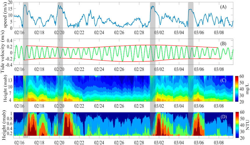
FIGURE 6. Time series of the wind speed (A), vertically averaged tidal current in the v-direction observed by ADCP (B), and SSC calculated via echo intensities measured by ADCP (C) and PC-ADP (D), respectively, during the winter of 2017. The gray shading indicates the strong wind events.

FIGURE 7. Time series of the wind speed (A), vertically averaged tidal current in the v-direction observed by ADCP (B), and SSC calculated via echo intensities measured by ADCP (C) and PC-ADP (D), respectively, during the summer of 2019.
In the four strong wind events during the winter 2017 observation period, a notable phenomenon occurred: many high-concentration bubbles extended from the upper to the middle parts, and even to the lower parts of the water bodies, as shown in Figure 6C. Similarly, during the summer 2019 observation period, after 20 August, the abrupt increase of the SSC in the upper layers of the water body may be related to the bubbles caused by the wind speed increase, as shown in Figure 7C. During the winter, after each strong wind event, the SSC increased sharply, the duration of the high SSC period often exceeded 24 h, and the tidal current only had a secondary effect on the SSC, as shown in Figure 6. During the summer 2019 observation period, no significant sediment resuspension occurred in the bottom boundary layer owing to the absence of strong wind events and, generally, the variation in SSC was consistent with tidal current changes, as shown in Figure 7.
Additionally, Figure 8 shows that the correlation between the SSC in the upper, middle, and lower layers and the SSC in the bottom layer was significantly different during the winter 2017 observation period and the summer 2019 observation period.
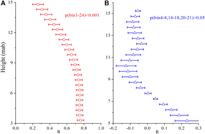
FIGURE 8. Mean (hollow circles/triangles) and standard deviation (error bars) of the correlation coefficients R between the SSC measured by the upward-looking ADCP and downward-looking PC-ADP during the winter of 2017 (A) and summer of 2019 (B).
The vertical distribution of the average correlation coefficients during the 2017 observation period is shown in Figure 8A. The mean value gradually increased with the water depth increasing, and its variation range was approximately 0.26–0.76.
Owing to the occurrence of strong wind events, the wave-induced shear stress at the bottom was greater than the critical bed shear stress of 0.16 Pa, resulting in bottom sediment resuspension (Jiang et al., 2020). With the depth increasing, the distance from the bottom decreased while the influence of bottom sediment resuspension increased. Hence, in the sea area off Qinhuangdao during the winter observation period, the sediment resuspension in the bottom layer played an important role in defining the SSC in the lower, middle, and upper layers.
The vertical distribution of the average correlation coefficients from the summer 2019 observation period is shown in Figure 8B, which varied from −0.13 to 0.23. The correlation coefficients from the 7th to the 21st bin of the ADCP were negative, whereas the values from the 1st to the 6th bin near the bottom boundary layer were positive. Moreover, the values increased gradually with depth from the 6th to the 1st bin. This suggests that in the summer, when no strong wind events occurred in the sea area off Qinhuangdao, the resuspension of seabed sediments had a negligible effect on the SSC in upper and middle layers, but had a certain contribution to the SSC in lower layers.
Overall, the winter SSC variations were significantly correlated with strong wind events, whereas the summer SSC variations were predominately controlled by tides and tidal currents.
The distinctive features on hydrodynamics and sediment dynamics described in results Section are as follows. Firstly, winter residual currents had a 10 h lag to the wind field, especially in such shallow coastal waters (Figures 5A, B). Secondly, the winter SSC variations were significantly correlated with strong wind events (Figures 6A, D), whereas the summer SSC variations were predominately controlled by tides and tidal currents (Figures 7B, D). Thirdly, the SSC in the upper, middle, and lower layers had a close relationship with the SSC in the bottom layer in winter, but not in summer (Figures 8A, B). The formation mechanism of these features will be explored in the following three parts, including the delayed response mechanism of residual current to wind field, the forcing analysis of kinetic factors through Reynolds stress and TKE in the bottom layer, and the impact ability of vertical circulation by suspended sediment flux decomposition.
The 10 h lag response of residual current and SSC to wind field in winter seems to be unreasonable for such shallow Bohai Sea with an average depth of 18 m. This strongly suggested that the residual current was not directly driven by local winds (wind stress). Similar time lag has been reported in Duan et al. (2020b) showing the 3–6 h lag, and Wang et al. (2020) indicating even more than 1 day lag on the deep side of the Bohai Strait. They both concluded that the time lag was most likely controlled by wind-triggered coastal trapped waves (CTWs). At the bay-shelf and estuary-shelf junction, such as the Bohai Strait, CTWs play an important role of water and sediment exchange (Wang et al., 2020). The study site located off the Qinhuangdao, different from the bay-shelf system might have a distinct mechanism. In order to better reveal the mechanism of the wind effect on the Bohai Sea circulation, the daily averaged SSH data from CMEMS and the wind data from ECMWF were applied in this study (Figure 9). And the availability of wind data from ECMWF has been demonstrated by data consistence, compared with measured wind speeds.
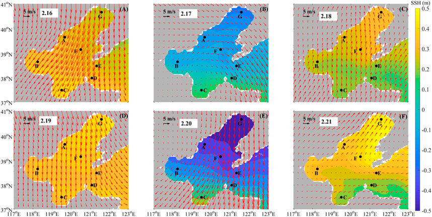
FIGURE 9. Spatial distribution of the 10 m wind field (vectors) and sea surface height (color shading) from February 16 to 21 (A–F), 2017.
Under the influence of East Asian Monsoon, the northerly wind prevails over the entire Bohai Sea and Yellow Sea in winter. Strong wind events could have a significantly impact on the redistribution of regional Sea Surface Height (SSH), and the response of SSH to strong wind events has a certain lag as well as, shown in Figure 9. During the first strong northerly wind event on 16th February, there was no significantly change in SSH (Figure 9A). When the wind relaxed even reversed on 17th February, the SSH in the entire Bohai Sea lowered significantly, with relatively low in the north and high in the south, as shown in Figure 9B. The change in SSH resulted in a north-south pressure gradient and northward compensation current (Hu et al., 2017). Correspondingly, the residual current increased significantly on 17 February, as shown in Figure 4B. On 18th February, the wind was southerly and the wind speed decreased, and the SSH began to rise (Figure 9C). The SSH reached its highest level on 19th February, as shown in Figure 9D, almost the entire SSH was higher than 0.3 m. The first strong northerly-relaxation-reversal-southerly wind round was over. From 19th February, the second similar round began(Figures 9E, F). Due to the stronger northerly wind than the first round, the change in SSH was more intense, as shown in Figure 9E.
Generally, the residual current was driven by winter strong wind using two approaches, direct wind stress and wind-triggered pressure gradient force in the shelf sea. Time series of wind speed and wind direction (Figure 10A), seawater acceleration generated by wind stress in U and V directions (Figure 10B), vertical mean residual current velocity (Figure 10C) at the study site, and seawater acceleration generated by pressure gradient force in V direction at 7 representative points (A-G) (Figure 10D) from 16 February to 21 February were illustrated. The pressure gradient force was calculated using the gradient of SSH (Figure 9). The response of wind stress to wind speed was real-time (in Figures 10A, B), while the response of residual current velocity and pressure gradient force to wind speed was hysteretic with the 10 h lag (Figures 10C, D). Furthermore, pressure gradient force-induced acceleration was larger than the wind stress-induced one. It could be concluded that the 10 h lag of residual current to wind speed was most likely dominated by the pressure gradient force, which generated by wind-driven SSH variations.
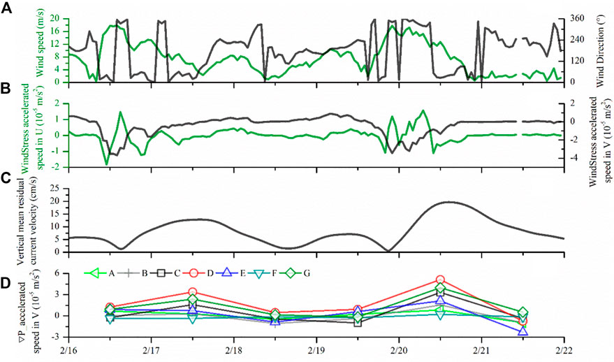
FIGURE 10. Time series of the wind speed and wind direction (A), the wind-induced seawater acceleration in U and V directions (B), the vertical mean residual current speed (C), and seawater acceleration generated by pressure gradient force in V direction at location points A-G (D) from February 16 to 21, 2017. The locations of points A-G are shown in the Figure 11, and the A point is located at the S1 mooring site. Among them, the figure (A–C) are from field observation data, and figure (D) is derived from CMEMS.
The 2017 Reynolds stress calculations using Eq. 4 yielded results close to those obtained by Jiang et al. (2020), who calculated the total bed shear stress, including wave-induced stress, current-induced stress, and wave-current interaction, as shown in Figure 11A. When the bottom shear stress caused by wave is much larger than that caused by current, the wave-current-induced bottom shear stress might be only slightly larger than that caused by wave itself (Yang et al., 2011). Owing to the shallow water depth in the Bohai Sea, the energetic waves could act straightly on the seabed, leading to active coastal erosion and resuspension (Wang et al., 2014; Zhao et al., 2022). In the sea area off Qinhuangdao, similar to other regions of the Bohai Sea, the wave-induced shear stress in winter invariably plays a primary role in sediment resuspension. Energetic waves would enhance the turbulence of sea water, which could be well expressed by Reynolds stress and TKE (shown as Figures 11, 12).
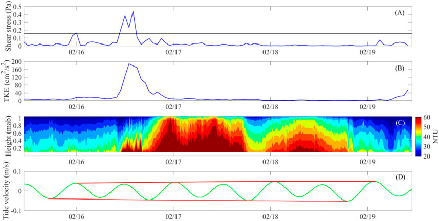
FIGURE 11. Time series of the Reynolds stress (A), TKE (B), SSC vertical profiles measured by the downward-looking PC-ADP (C), and the V component of the tidal current at 0.1 mab (D) from 11:00 on 15 February 2017 to 11:00 on 19 February 2017.
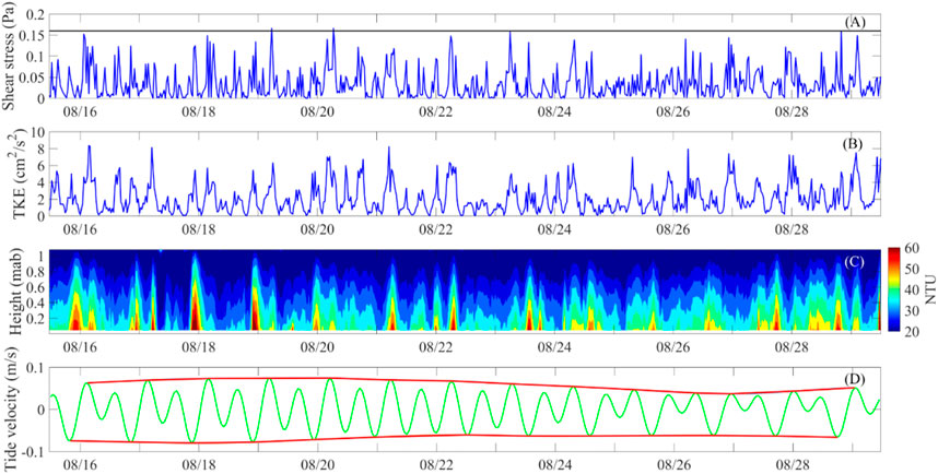
FIGURE 12. Time series of the Reynolds stress (A), TKE (B), SSC vertical profiles measured by the downward-looking PC-ADP (C), and the V component of the tidal current at 0.1 mab (D) during the summer of 2019.
Jiang et al. (2020) evaluated the critical bed shear stress as 0.16 Pa considering the cohesive characteristics of seabed sediments, which was closed to the sand critical shear stress of 0.14 Pa (Wang et al., 2020), indicating that the fraction of sand in the sea area off Qinhuangdao was relatively high. The black line in Figures 11A, 12A represents the value of the critical bed shear stress. At 10:00 on 16 February 2017, the wind speed exceeded 14 m/s, and the Reynolds stress reached its first peak value (0.38 Pa) at 12:00, and reached the maximum value (0.44 Pa) at 14:00, which exceeded by far the critical stress of 0.16 Pa and lower than the maximum shear stress of 0.5 Pa under wave-current interaction during storm buildup phase in the Bohai Strait in winter 2018 (Wang et al., 2020). Similarly, Duan et al. (2020b) discovered that the wave shear stress at the bottom of Bohai Strait was about 0.5 Pa during the winter strong wind event. Acting as the other crucial dynamic parameter, the TKE was increasing significantly, reaching its maximum value (188 cm2/s2) at 13:00 (Figure 11B). MacVean and Lacy (2014) proposed that the TKE generally remained below 50 cm2/s2 under tidal influence alone, but exceed 100 cm2/s2 during the major wind event. Due to high Reynolds stress and TKE, significant sediment resuspension occurred, resulting in a swift increase in SSC, as shown in Figure 11C.
Figure 11D shows the time series of the V component of tidal currents at 0.1 mab, which barely changed before and after the massive sediment resuspension; therefore, in the winter, with strong wind events, the tidal current did not have a major effect on the SSC in the bottom layer. In August 2019, the Reynolds stress was mostly less than the critical bed shear stress of 0.16 Pa, as shown in Figure 12A, and all TKE values were lower than 10 cm2/s2, and less than a 10th of the maximum TKE from winter 2017, as shown in Figure 12B. The weak Reynolds stress and low TKE could not trigger the resuspension of bed sediments, which had little influence on the variation of the SSC. The correlation coefficient between the SSC at 0.1 mab and the TKE was smaller than 0.1, which further demonstrated that the SSC were independent of the wind-induced turbulence.
It can be seen from Figures 12C, D that the increase of high SSC and the change of tidal current velocity in V component at 0.1 mab have obvious tidal periodic signals. More specifically, the period of the SSC varied with the difference of the diurnal inequality pattern (Figures 12C, D), indicated by sectional spectrum analysis. Before 19 August, the significant SSC period was 8 h due to the evident diurnal inequality. From then until 25 August, the significant SSC periods were 6 and 8 h since the semi-diurnal tidal currents were almost equal. After 25 August, the diurnal inequality was more pronounced, so the corresponding SSC had cycles of 8 and 12 h. Since the corresponding Reynolds stress during the summer observation period was mostly lower than the critical stress, the advection transport of tidal currents may be the main reason for the variation of SSC. Ultimately, in the summer, without strong wind events, the tidal currents played a major role on the SSC in the bottom layer.
Eq. 8 was used to calculate the tidally-averaged suspended sediment flux [F, g/(m s)], following the method used by (Dyer, 1997). The U component in the east-west direction and the V component in the north-south direction were calculated, and the positive sediment flux values represented the east or north direction. The results of the horizontal decomposition terms (F1–F5) and vertical circulation effects terms (F6–F7) in 2017 and 2019 are shown in Tables 2, 3, respectively.
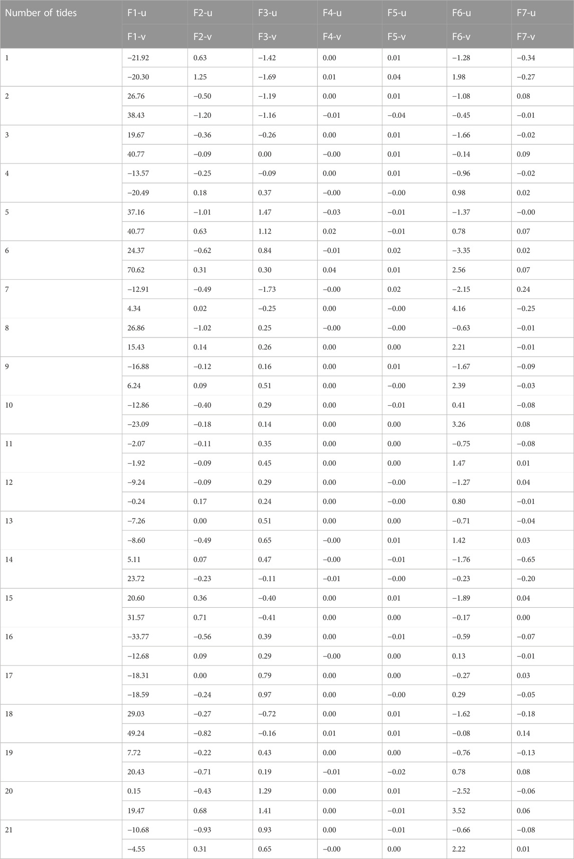
TABLE 2. Tidally averaged suspended sediment flux [F, g/(m s)] and its decomposition terms (F1-F7) at S1 in 2017. Among them, -u is the component of F in the east-west direction, and a positive value indicates east; -v is the component of F in the north-south direction, and a positive value indicates north.

TABLE 3. Tidally averaged suspended sediment flux [F, g/(m s)] and its decomposition terms (F1–F7) at S1 in 2019. Among them, -u is the component of F in the east-west direction, and a positive value indicates east; -v is the component of F in the north-south direction, and a positive value indicates north.
The time series of the decomposition terms (F1+F2, F3+F4+F5, F6+F7) of the tidally-averaged suspended sediment flux (F) in the U and V directions at S1 in 2017 and 2019 are shown in Figure 13.
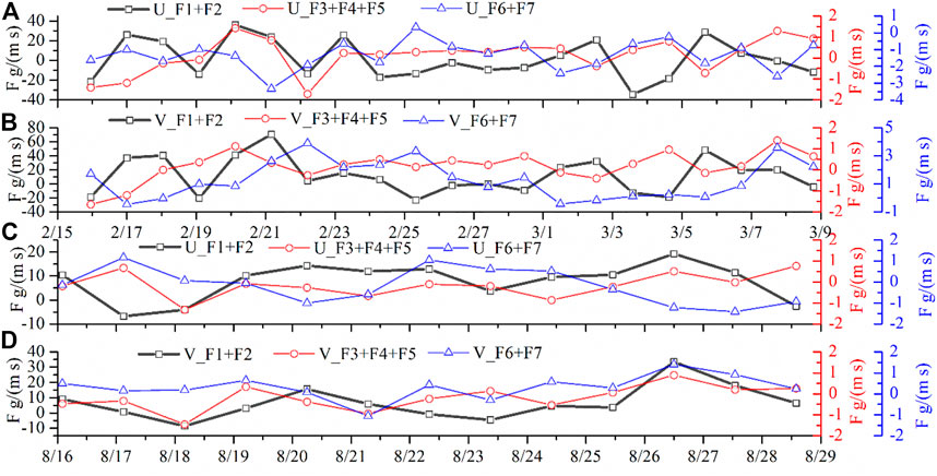
FIGURE 13. Time series of the advection terms (F1+F2), tidal pumping terms (F3+F4+F5), and vertical circulation effect terms (F6+F7) at S1 in the U direction (A,C) and V direction (B,D) during the winter of 2017 (A,B) and summer of 2019 (C,D).
As shown in Figure 13; Tables 2, 3, the main contributor of F in the sea area off Qinhuangdao was its decomposition term F1, indicating that dominant currents played the most important contribution to suspended sediment transport during the two observation periods. Qiao et al. (2010) also proposed that residual currents were key hydrodynamic factors controlling sediment distribution and transport in the Bohai Sea. During the winter and summer observation periods, the average suspended sediment fluxes in the U and V directions were 0.30 ± 19.29 g/(m s) and 13.46 ± 25.34 g/(m s) in 2017, and 7.44 ± 7.16 g/(m s) and 6.81 ± 11.12 g/(m s) in 2019. These fluxes were far smaller than the SSF in the sea area off the Huanghe Delta, where the average SSF in winter were about 8,000 g/(m s) in winter and about 2,700 g/(m s) in summer due to super high SSC (Yang et al., 2011). Additionally, the average SSF during the winter observation period was less than the output of 51.2 g/(m s) through the southern side of the Bohai Strait during intense northerly wind event in the winter of 2018, which was the only pathway for Huanghe-derived sediments transported to the Yellow Sea (Duan et al., 2020b). Whereas during the winter observation period, the average SSF in the V direction was almost in the same order of magnitude as the winter SSF in the southern Yellow Sea, where cross-shelf transportation occurred from the Old Huanghe Delta to the shelf edge (Pang et al., 2020). As shown in Figures 13; Tables 2, 3, the range of variation of the tidally-averaged SSF was larger in winter than that in summer, which was consistent with the seasonal comparison of the SSF at the Huanghe Delta by Yang et al. (2011), and on the south part of the Bohai Sea by Wang et al. (2014).
As shown in Figure 13, the net direction of suspended sediment transport was northeastward in the summer, as it benefited the alongshore transport of river-derived suspended sediment in the south of the Qinhuangdao. Conversely, in winter, the suspended sediment was transported towards the northeast during the strong wind events, then towards the southwest in the intermittent period of strong winds. This back-and-forth transport led to a small net northward sediment flux, which might be the fundamental reason of the low SSC sustaining for the whole winter in the study site. Analogous back-and-forth transport through the Bohai Strait was demonstrated using two bottom-mounted platforms’ observations by Duan et al. (2020b), and reproduced by a high-resolution model in Wang et al. (2020). Those studies and our research have all focused on the typical winter synoptic event, consisting of strong northerly wind, relaxation, reversal, and weak southerly wind.
To quantify the contribution of advection transport terms (F1+F2), tidal pumping terms (F3+F4+F5), and vertical circulation effect terms (F6+F7) to the SSF, the proportion of the absolute value of each term was calculated. During the winter 2017 observation period, the ratios of advection transport terms, tidal pumping terms, and vertical circulation effect terms to SSF in the U direction were 0.84 ± 0.18, 0.05 ± 0.06, and 0.11 ± 0.13, respectively. In the V direction, the corresponding ratios were 0.83 ± 0.19, 0.04 ± 0.04, and 0.13 ± 0.16, respectively. However, during the summer 2019 observation period, the ratios of advection transport, tidal pump, and vertical circulation effect to SSF in the U direction were 0.87 ± 0.01, 0.06 ± 0.07, and 0.07 ± 0.06, respectively. In the V direction, the corresponding ratios were 0.85 ± 0.11, 0.07 ± 0.05, and 0.08 ± 0.07, respectively.
By calculating the proportion of each term in SSF, we proved that the advection transport terms had the largest contribution (80%) to the SSF, regardless of the season. The tidal pumping terms were relatively small, fluctuating between 4% and 7%, which may be caused by the study site being adjacent to an amphidromic point. The proportion of vertical circulation effect terms fluctuated between 7% and 13%, with a ratio greater than 0.1 in the winter and less than 0.1 in the summer, indicating that strong wind events in the winter strengthened the vertical exchange of suspended sediment. Additionally, during the 2017 observation period, the mean values of the sum of the F6 and F7 values were 1.41 ± 0.78 g/(m s) and 1.50 ± 0.23 g/(m s) in the U and the V directions, respectively, which were larger than those of the 2019 observation period (0.73 ± 0.42 g/(m s) and 0.57 ± 0.36 g/(m s), respectively). This further proved that the vertical circulation intensity in the winter was greater than that in the summer. Accordingly, the correlation between the SSC in the upper-middle layers and in the bottom layer in the winter was more evident than it was in the summer (Figure 8).
Through the above discussion, the delayed response of residual current to wind field, the importance of the Reynolds stress and TKE for sediment resuspension, and the impact of vertical circulation on suspended sediment flux might be explained in principle. Driven by the pressure gradient force associated with the wind-induced sea surface height variations, the winter current was closely related to the wind speed with a time lag of 10 h. Different from the strong-wind-dominated winter SSC, summer SSC variations were mainly controlled by tides and tidal currents. Impact of vertical circulation on SSC was twice stronger in winter than summer.
Moreover, the phenomenon of delayed response to strong winds not only occurred in the sea area off Qinhuangdao, but also widely exists in other coastal areas. Münchow and Garvine (1993) displayed that the across-shelf flow component (10 m below the surface) lagged the same along-shore wind for 6 h after analyzing the observation data at the mouth of the Delaware Estuary on the East Coast of the United States. Skagseth et al. (2011) manifested that in the Barents Sea of the Arctic Ocean, the principal component of the residual current empirical orthogonal function (EOF) mode lagged the along-coast wind for about 6 h. Li et al. (2015) pointed out that in the Grand Banks of Newfoundland on the East Coast of Canada with an average depth of only 10 m, the wave peak still lagged the wind speed by 2 h, meanwhile storm-induced surface currents often lagged the wind by several hours. And the high concentration of suspended sediment appeared to lag behind the high wind speed by about 2 h at the Gooses Reef station in Chesapeake Bay on the East Coast of the United States by Xie et al. (2018). In the Bohai Strait adjacent to the study area, the correlation coefficient between the north-south component of sea surface wind and sea level anomaly was 0.82, and the lag time of sea level anomaly to sea surface wind was 15 h (Ding et al., 2019). In addition, if the water depth is too shallow, the delayed response to wind speed is not significant. Since the Chincoteague Bay on the East Coast of the United States had an average depth of 1.4 m, and wind could generate waves promptly, there was little lag between energy input from the wind and its corresponding wave-height response (Nowacki and Ganju, 2018). The lag time of responding the wind field was different depending on factors such as local water depth, wind speed and the angle between wind and sea surface. Different from the pressure gradient force lagging strong winds and dominating the residual current in this study, wind-triggered trapped waves probably modulated the lag phenomenon, e.g., continental trapped waves in Skagseth et al. (2011), coastal trapped waves in Ding et al. (2019), Duan et al. (2020b) and Wang et al. (2020).
Generally speaking, the strong wind-driven stress is large enough to mix the water column, further strengthening the vertical exchange of sediments (Chen and Sanford, 2009; Yang et al., 2011). The contribution of the vertical circulation effect term to the suspended sediment flux in the Qinhuangdao sea area was two times greater in winter than in summer, mainly because there occurred more strong wind events in winter, which was applicable to other shallow coastal waters. Zhou et al. (2021) revealed that strong winds and their induced waves were crucial for the resuspension and transport of sediment in the Yangtze River Estuary in the East China Sea. In the Gulf of Lions of the western Mediterranean Sea, strong sediment transport events occurred during the storms (Palanques et al., 2006). Through the idealized experiments, it was found that the lateral suspended sediment fluxes during strong winds were larger than those during moderate winds, because strong winds led to larger bottom shear stress, stronger lateral flows and weaker stratification in an idealized, partially mixed estuary (Chen et al., 2009).
A seabed base observation platform was deployed in the sea area off Qinhuangdao for 22 days in February 2017 and 14 days in August 2019. In this study, the mooring measurements were used to examine the features of the hydrodynamic environment and SSF at the study site in both winter and summer for better understanding the circulation structure and sediment exchange in the Bohai Sea.
In summer, the seawater had higher temperature, lower salinity (with slight variations), and lower SSC (under low-wind conditions) than in winter. In summer, the residual currents, predominantly flowing northeastward, were relatively small and exhibited little correlation with the wind speed except for the surface and bottom layers. In winter, residual currents flowed to the northeast during strong wind periods and primarily to the southwest during intermittent periods. This back-and-forth current only led to a small net sediment transport, which might be the fundamental reason of the low SSC sustaining in the study site in winter.
During the 2017 observations, the correlations between the wind speed and 10 h lag residual current were the most significant, mostly between ∼0.4 and 0.6. Winter strong winds could drive residual currents through direct wind stress and wind-triggered pressure gradient force, and the action of wind stress real-time responding to wind field was less than the action of pressure gradient force 10 h lag responding to wind field. Thus, the winter residual currents at the study site were dominated by the pressure gradient force generated by wind-driven sea surface height variations, leading to the 10 h lag response to wind speed. In winter, after the occurrence of each strong wind event, the SSC increased sharply and the duration of the high SSC period often exceeded 24 h. On the contrary, SSC variations in summer were consistent with changes in tidal currents.
During strong winter wind periods, large Reynolds stress and high TKE cause a significant sediment resuspension, resulting in a swift increase in SSC in the middle-upper layers of water bodies. In the summer, owing to low wind speeds, weak Reynolds stress, and low TKE, the resuspension of bed sediments was not triggered, resulting in little correlation between the SSC changes in the middle-upper layers and that in the bottom layer. The increase of SSC in summer may be mainly due to the advection transport of tidal current. Specifically, the period of SSC varied with the difference of tidal diurnal inequality patterns. The SSF decomposition showed that the dominant advection played the most important contribution to suspended sediment transport, followed by the vertical circulation, while the tidal pumping contributed the least owing to its adjacency to an amphidromic point, regardless of the season. The flux decomposition further indicated that the impact of the vertical circulation on the sediment flux in winter was two times stronger than that in summer.
The lag time of responding the wind field would vary with local water depth, wind speed, etc. In this study, the delayed response to the wind was mainly due to the pressure gradient force lagging strong winds and dominating the residual current. This explanation could provide a reference for other coastal waters. Strong winds could enhance the vertical suspended sediment flux. The contribution of vertical circulation terms to suspended sediment flux in winter being greater than that in summer might have certain applicability in other monsoon-dominating shelf seas.
The original contributions presented in the study are included in the article/supplementary material, further inquiries can be directed to the corresponding author.
DZ: data analysis, writing original draft. CP: conceptualization, methodology, supervision, validation. ZL: investigation. JJ: investigation.
This work was supported by the Scientific Instrument Developing Project of the Chinese Academy of Sciences (Project No. YJKYYQ20190047), the National Natural Science Foundation of China (Project No. 41576060) and Hebei Science and Technology Project (Grant No. 19273301D).
The authors thank all of the investigators for their help in collecting samples and data during the field survey. I would like to thank the three reviewers for their constructive comments and suggestions, which have improved the contents and clarity of this paper. Thanks to Dr. Xiaomei Yan for helping improve the paper. Thanks to the Chief Editor Valerio Acocella for comments and suggestions, which have greatly improved our work.
The authors declare that the research was conducted in the absence of any commercial or financial relationships that could be construed as a potential conflict of interest.
All claims expressed in this article are solely those of the authors and do not necessarily represent those of their affiliated organizations, or those of the publisher, the editors and the reviewers. Any product that may be evaluated in this article, or claim that may be made by its manufacturer, is not guaranteed or endorsed by the publisher.
Bian, C. W., Jiang, W. S., Greatbatch, R. J., and Ding, H. (2013). The suspended sediment concentration distribution in the Bohai Sea, Yellow Sea and east China sea. J. Ocean. Univ. Chin. 12, 345–354. doi:10.1007/s11802-013-1916-3
Birch, G. F., Eyre, B., and Taylor, S. E. (1999). The distribution of nutrients in bottom sediments of Port Jackson (Sydney Harbour), Australia. Mar. Pollut. Bull. 38, 1247–1251. doi:10.1016/S0025-326x(99)00184-8
Chen, S. N., and Sanford, L. P. (2009). Axial wind effects on stratification and longitudinal salt transport in an idealized, partially mixed estuary. J. Phys. Oceanogr. 39, 1905–1920. doi:10.1175/2009JPO4016.1
Chen, S. N., Sanford, L. P., and Ralston, D. K. (2009). Lateral circulation and sediment transport driven by axial winds in an idealized, partially mixed estuary. J. Geophys. Res. Oceans 114, C12006. doi:10.1029/2008jc005014
Chen, X. L., Lu, J. Z., Cui, T. W., Jiang, W. S., Tian, L. Q., Chen, L. Q., et al. (2010). Coupling remote sensing retrieval with numerical simulation for SPM study-Taking Bohai Sea in China as a case. Int. J. Appl. Earth. Obs. 12, S203–S211. doi:10.1016/j.jag.2009.10.002
Cui, T. W., Zhang, J., Ma, Y., Zhao, W. J., and Sun, L. (2009). The study on the distribution of suspended particulate matter in the Bohai Sea by remote sensing. Acta Oceanol. Sin. 31, 10–18. (in Chinese with English abstract).
de Nijs, M. A. J., Winterwerp, J. C., and Pietrzak, J. D. (2009). On harbour siltation in the fresh-salt water mixing region. Cont. Shelf Res. 29, 175–193. doi:10.1016/j.csr.2008.01.019
Ding, Y., Bao, X. W., Yao, Z. G., Bi, C. C., Wan, K., Bao, M., et al. (2019). Observational and model studies of synoptic current fluctuations in the Bohai Strait on the Chinese continental shelf. Ocean. Dynam 69, 323–351. doi:10.1007/s10236-019-01247-5
Duan, H. Q., Wang, C. H., Liu, Z. Q., Wang, H. J., Wu, X., and Xu, J. P. (2020a). Summer wind gusts modulate transport through a narrow strait, Bohai, China. Estuar. Coast Shelf Sci. 233, 106526. doi:10.1016/J.Ecss.2019.106526
Duan, H. Q., Xu, J. P., Wu, X., Wang, H. L., Liu, Z. Q., and Wang, C. H. (2020b). Periodic oscillation of sediment transport influenced by winter synoptic events, Bohai Strait, China. Water 12, 986. doi:10.3390/w12040986
Dyer, K. R., Christie, M. C., Feates, N., Fennessy, M. J., Pejrup, M., and van der Lee, W. (2000). An investigation into processes influencing the morphodynamics of an intertidal mudflat, the dollard estuary, The Netherlands: I. Hydrodynamics and suspended sediment. Estuar. Coast Shelf Sci. 50, 607–625. doi:10.1006/ecss.1999.0596
Dyer, K. R. (1997). Estuaries-A physical introduction. 2nd ed. Chichester, U.K: John Wiley, 195. doi:10.1017/s0025315400041825
Elias, E. P. L., van der Spek, A. J. F., Wang, Z. B., and de Ronde, J. (2012). Morphodynamic development and sediment budget of the Dutch Wadden Sea over the last century. Neth J. Geosci. 91, 293–310. doi:10.1017/s0016774600000457
Erikson, L. H., Wright, S. A., Elias, E., Hanes, D. M., Schoellhamer, D. H., and Largier, J. (2013). The use of modeling and suspended sediment concentration measurements for quantifying net suspended sediment transport through a large tidally dominated inlet. Mar. Geol. 345, 96–112. doi:10.1016/j.margeo.2013.06.001
Ganju, N. K., Schoellhamer, D. H., and Bergamaschi, B. A. (2005). Suspended sediment fluxes in a tidal wetland: Measurement, controlling factors, and error analysis. Estuaries 28, 812–822. doi:10.1007/Bf02696011
Hu, Z. F., Wang, D. P., He, X. Q., Li, M. T., Wei, J., Pan, D. L., et al. (2017). Episodic surface intrusions in the Yellow Sea during relaxation of northerly winds. J. Geophys. Res. Oceans 122, 6533–6546. doi:10.1002/2017JC012830
Huang, D. J., Su, J. L., and Backhaus, J. O. (1999). Modelling the seasonal thermal stratification and baroclinic circulation in the Bohai Sea. Cont. Shelf Res. 19, 1485–1505. doi:10.1016/S0278-4343(99)00026-6
Jiang, W. S., Pohlmann, T., Sun, J., and Starke, A. (2004). SPM transport in the Bohai Sea: Field experiments and numerical modelling. J. Mar. Syst. 44, 175–188. doi:10.1016/j.jmarsys.2003.09.009
Jiang, M., Pang, C., Liu, Z., and Jiang, J. (2020). Sediment resuspension in winter in an exceptional low suspended sediment concentration area off Qinhuangdao in the Bohai Sea. Estuar. Coast. Shelf Sci. 245, 106859. doi:10.1016/j.ecss.2020.106859
Kularatne, S., and Pattiaratchi, C. (2008). Turbulent kinetic energy and sediment resuspension due to wave groups. Cont. Shelf Res. 28, 726–736. doi:10.1016/j.csr.2007.12.007
Lee, E. M., Bowers, D. G., and Kyte, E. (2009). Remote sensing of temporal and spatial patterns of suspended particle size in the Irish Sea in relation to the Kolmogorov microscale. Cont. Shelf Res. 29, 1213–1225. doi:10.1016/j.csr.2009.01.016
Li, J. F., and Zhang, C. (1998). Sediment resuspension and implications for turbidity maximum in the Changjiang Estuary. Mar. Geol. 148, 117–124. doi:10.1016/S0025-3227(98)00003-6
Li, G. S., Wang, H. L., and Liao, H. P. (2010). Numerical simulation on seasonal transport variations and mechanisms of suspended sediment discharged from the Yellow River to the Bohai Sea. J. Geogr. Sci. 20, 923–937. doi:10.1007/s11442-010-0821-6
Li, M. Z., Wu, Y. S., Prescott, R. H., Tang, C. C. L., and Han, G. Q. (2015). A modeling study of the impact of major storms on waves, surface and near-bed currents on the Grand Banks of Newfoundland. J. Geophys. Res. Oceans 120, 5358–5386. doi:10.1002/2015JC010755
Li, Y., Jia, J. J., Zhu, Q. G., Cheng, P., Gao, S., and Wang, Y. P. (2018). Differentiating the effects of advection and resuspension on suspended sediment concentrations in a turbid estuary. Mar. Geol. 403, 179–190. doi:10.1016/j.margeo.2018.06.001
Liu, G. M., Wang, H., Sun, S., and Han, B. P. (2003). Numerical study on density residual currents of the Bohai sea in summer. Chin. J. Oceanol. Limnol. 21 (2), 106–113.
Liu, X. M., Qiao, L. L., Zhong, Y., Wan, X. Q., Xue, W. J., and Liu, P. (2020a). Pathways of suspended sediments transported from the Yellow River mouth to the Bohai Sea and Yellow Sea. Estuar. Coast. Shelf Sci. 236, 106639. doi:10.1016/J.Ecss.2020.106639
Liu, X. M., Qiao, L. L., Zhong, Y., Xue, W. J., and Liu, P. (2020b). Multi-year winter variations in suspended sediment flux through the Bohai Strait. Remote Sens. 12, 4066. doi:10.3390/Rs12244066
Liu, H. W., Pang, C. G., Yang, D. Z., and Liu, Z. L. (2021). Seasonal variation in material exchange through the Bohai Strait. Cont. Shelf Res. 231, 104599. doi:10.1016/J.Csr.2021.104599
Loisel, H., Mangin, A., Vantrepotte, V., Dessailly, D., Dinh, D. N., Garnesson, P., et al. (2014). Variability of suspended particulate matter concentration in coastal waters under the Mekong's influence from ocean color (MERIS) remote sensing over the last decade. Remote Sens. Environ. 150, 218–230. doi:10.1016/j.rse.2014.05.006
MacVean, L. J., and Lacy, J. R. (2014). Interactions between waves, sediment, and turbulence on a shallow estuarine mudflat. J. Geophys. Res. Oceans 119, 1534–1553. doi:10.1002/2013JC009477
Mao, X. Y., Wang, D. S., Zhang, J. C., Bian, C. W., and Lv, X. Q. (2018). Dynamically constrained interpolation of the sparsely observed suspended sediment concentrations in both space and time: A case study in the Bohai Sea. J. Atmos. Ocean. Technol. 35, 1151–1167. doi:10.1175/Jtech-D-17-0149.1
Meirelles, S., Henriquez, M., Horner-Devine, A. R., Souza, A. J., Pietrzak, J., and Stive, M. (2015). “Bed shear stress on the middle shoreface of the south-holland coast,” in The proceedings of the coastal sediments 2015. doi:10.1142/9789814689977_0210
Münchow, A., and Garvine, R. W. (1993). Buoyancy and wind forcing of a coastal current. J. Mar. Res. 51, 293–322. doi:10.1357/0022240933223747
Muslim, I., and Jones, G. (2003). The seasonal variation of dissolved nutrients, chlorophyll a and suspended sediments at Nelly Bay, Magnetic Island. Magn. Isl. Estuar. Coast Shelf Sci. 57, 445–455. doi:10.1016/S0272-7714(02)00373-6
Nowacki, D. J., and Ganju, N. K. (2018). Storm impacts on hydrodynamics and suspended-sediment fluxes in a microtidal back-barrier estuary. Mar. Geol. 404, 1–14. doi:10.1016/j.margeo.2018.06.016
Nowacki, D. J., Ogston, A. S., Nittrouer, C. A., Fricke, A. T., and Tri, V. P. D. (2015). Sediment dynamics in the lower Mekong River: Transition from tidal river to estuary. J. Geophys. Res. Oceans 120, 6363–6383. doi:10.1002/2015JC010754
Oey, L. Y., Ezer, T., Wang, D. P., Fan, S. J., and Yin, X. Q. (2006). Loop current warming by hurricane wilma. Geophys. Res. Lett. 33, L08613. doi:10.1029/2006gl025873
Palanques, A., de Madron, X. D., Puig, P., Fabres, J., Guillen, J., Calafat, A., et al. (2006). Suspended sediment fluxes and transport processes in the Gulf of Lions submarine canyons. The role of storms and dense water cascading. Mar. Geol. 234, 43–61. doi:10.1016/j.margeo.2006.09.002
Pang, C. G., and Yu, W. (2013). Spatial modes of suspended sediment concentration in surface water in Bohai Sea and their temporal variations. Adv. Water Sci. 24, 722–727. (in Chinese with English abstract).
Pang, C. G., Yuan, D. L., Jiang, M., Chu, F. S., and Li, Y. (2020). Observed cross-shelf suspended sediment flux in the southern Yellow Sea in winter. Mar. Geol. 419, 106067. doi:10.1016/J.Margeo.2019.106067
Qiao, S. Q., Shi, X. F., Zhu, A. M., Liu, Y. G., Bi, N. S., Fang, X. S., et al. (2010). Distribution and transport of suspended sediments off the Yellow River (Huanghe) mouth and the nearby Bohai Sea. Estuar. Coast. Shelf Sci. 86, 337–344. doi:10.1016/j.ecss.2009.07.019
Qiao, L. L., Wang, Y. Z., Li, G. X., Deng, S. G., Liu, Y., and Mu, L. (2011). Distribution of suspended particulate matter in the northern Bohai Bay in summer and its relation with thermocline. Estuar. Coast Shelf Sci. 93, 212–219. doi:10.1016/j.ecss.2010.10.027
Qiao, L. L., Liu, S. D., Xue, W. J., Liu, P., Hu, R. J., Sun, H. F., et al. (2020). Spatiotemporal variations in suspended sediments over the inner shelf of the East China Sea with the effect of oceanic fronts. Estuar. Coast Shelf Sci. 234, 106600. doi:10.1016/J.Ecss.2020.106600
Shi, Z., Xu, J., Huang, X. P., Zhang, X., Jiang, Z. J., Ye, F., et al. (2017). Relationship between nutrients and plankton biomass in the turbidity maximum zone of the Pearl River Estuary. J. Environ. Sci. 57, 72–84. doi:10.1016/j.jes.2016.11.013
Skagseth, Ø., Drinkwater, K. F., and Terrile, E. (2011). Wind- and buoyancy-induced transport of the Norwegian coastal current in the Barents Sea. J. Geophys. Res. Oceans 116, C08007. doi:10.1029/2011jc006996
Soulsby, R. L., and Humphery, J. D. (1990). “Filed Observation of wave-current interaction at the sea bed,” in Water wave kinematics. Editors A. Torum, and O. T. Gudmestad (Dordrecht: Kluwer Academic Publishers), 413–428. doi:10.1007/978-94-009-0531-3_25
Su, J. L., and Wang, K. S. (1986). The suspended sediment balance in changjiang estuary. Estuar. Coast. Shelf Sci. 23, 81–98. doi:10.1016/0272-7714(86)90086-7
Uncles, R. J., Elliott, R. C. A., and Weston, S. A. (1985a). Dispersion of salt and suspended sediment in a partly mixed estuary. Estuaries 8, 256–269. doi:10.2307/1351486
Uncles, R. J., Elliott, R. C. A., and Weston, S. A. (1985b). Observed fluxes of water, salt and suspended sediment in a partly mixed estuary. Estuar. Coast. Shelf Sci. 20, 147–167. doi:10.1016/0272-7714(85)90035-6
Wang, W. J., and Jiang, W. S. (2008). Study on the seasonal variation of the suspended sediment distribution and transportation in the East China Seas based on SeaWiFS data. J. Ocean. Univ. Chin. 7, 385–392. doi:10.1007/s11802-008-0385-6
Wang, H. L., and Li, G. S. (2009). Numerical simulation on seasonal transportation of suspended sediment from Huanghe (Yellow) river to Bohai Sea. Oceanol. Limnol. Sin. 40, 129–137. (in Chinese with English abstract).
Wang, H. J., Bi, N. S., Saito, Y., Wang, Y., Sun, X. X., Zhang, J., et al. (2010). Recent changes in sediment delivery by the Huanghe (Yellow River) to the sea: Causes and environmental implications in its estuary. J. Hydrol. 391, 302–313. doi:10.1016/j.jhydrol.2010.07.030
Wang, H. J., Wang, A. M., Bi, N. H., Zeng, X. M., and Xiao, H. H. (2014). Seasonal distribution of suspended sediment in the Bohai Sea, China. Cont. Shelf Res. 90, 17–32. doi:10.1016/j.csr.2014.03.006
Wang, Z., Qiao, L. L., Wang, Y. F., Liu, C., Tang, X., Zhang, H., et al. (2016). The optimization of fermentation conditions and enzyme properties of Stenotrophomonas maltophilia for protease production. Acta Sedimentol. Sin. 34, 292–299. (in Chinese with English abstract). doi:10.1002/bab.1361
Wang, C. H., Liu, Z. Q., Harris, C. K., Wu, X., Wang, H. J., Bian, C. W., et al. (2020). The impact of winter storms on sediment transport through a narrow strait, Bohai, China. J. Geophys. Res. Oceans 125 (6), 2169–9291. doi:10.1029/2020jc016069
Wei, J. W., Wang, M. H., Jiang, L. D., Yu, X. L., Mikelsons, K., and Shen, F. (2021). Global estimation of suspended particulate matter from satellite ocean color imagery. J. Geophys. Res. Oceans 126, e2021JC017303. doi:10.1029/2021JC017303
Wu, J. X., Shen, H. T., and Xiao, C. Y. (2001). Sediment classification and estimation of suspended sediment fluxes in the Changjiang Estuary, China. Water Resour. Res. 37, 1969–1979. doi:10.1029/2000wr900352
Wu, D. X., Wan, X. Q., Bao, X. W., Mu, L., and Lan, J. (2004). Comparison of summer thermohaline field and circulation structure of the Bohai Sea between 1958 and 2000. Chin. Sci. Bull. 49, 363–369. doi:10.1360/03wd0285
Wu, X., Xu, J. P., Wu, H., Bi, N. S., Bian, C. W., Li, P. H., et al. (2019). Synoptic variations of residual currents in the Huanghe (Yellow River)-derived distal mud patch off the Shandong Peninsula: Implications for long-term sediment transport. Mar. Geol. 417, 106014. doi:10.1016/J.Margeo.2019.106014
Xiao, Y., Wu, Z., Cai, H. Y., and Tang, H. W. (2018). Suspended sediment dynamics in a well-mixed estuary: The role of high suspended sediment concentration (SSC) from the adjacent sea area. Estuar. Coast. Shelf Sci. 209, 191–204. doi:10.1016/j.ecss.2018.05.018
Xie, X. H., Li, M., and Ni, W. F. (2018). Roles of wind-driven currents and surface waves in sediment resuspension and transport during a tropical storm. J. Geophys. Res. Oceans 123, 8638–8654. doi:10.1029/2018JC014104
Yang, Z. S., Ji, Y. J., Bi, N. S., Lei, K., and Wang, H. J. (2011). Sediment transport off the Huanghe (Yellow River) delta and in the adjacent Bohai Sea in winter and seasonal comparison. Estuar. Coast. Shelf Sci. 93, 173–181. doi:10.1016/j.ecss.2010.06.005
Yu, Q., Wang, Y. P., Flemming, B., and Gao, S. (2012). Tide-induced suspended sediment transport: Depth-averaged concentrations and horizontal residual fluxes. Cont. Shelf Res. 34, 53–63. doi:10.1016/j.csr.2011.11.015
Yu, Q., Wang, Y. W., Gao, J. H., Gao, S., and Flemming, B. (2014). Turbidity maximum formation in a well-mixed macrotidal estuary: The role of tidal pumping. J. Geophys. Res. Oceans 119, 7705–7724. doi:10.1002/2014JC010228
Yuan, D. L., Zhu, J. R., Li, C. Y., and Hu, D. X. (2008). Cross-shelf circulation in the Yellow and East China Seas indicated by MODIS satellite observations. J. Mar. Syst. 70, 134–149. doi:10.1016/j.jmarsys.2007.04.002
Zhao, G. B., Jiang, W. S., Wang, T., Chen, S. G., and Bian, C. W. (2022). Decadal variation and regulation mechanisms of the suspended sediment concentration in the Bohai Sea, China. J. Geophys. Res. Oceans 127. doi:10.1029/2021JC017699
Zhou, Z., Zhang, W. L., Jiang, W. S., Wang, X., and Bian, C. W. (2017). Long-term variation of suspended sediment concentration in the Bohai Sea based on retrieved satellite data. Periodical Ocean Univ. China 47, 10–18. (in Chinese with English abstract).
Zhou, Z. Y., Ge, J. Z., van Maren, D. S., Wang, Z. B., Kuai, Y., and Ding, P. X. (2021). Study of sediment transport in a tidal channel-shoal system: Lateral effects and slack-water dynamics. J. Geophys. Res. Oceans 126. doi:10.1029/2020JC016334
Keywords: sedimentary dynamic process, winter and summer observations, residual currents, suspended sediment flux decomposition, sea area off Qinhuangdao, the Bohai Sea
Citation: Zhang D, Pang C, Liu Z and Jiang J (2023) Winter and summer sedimentary dynamic process observations in the sea area off Qinhuangdao in the Bohai Sea, China. Front. Earth Sci. 11:1097033. doi: 10.3389/feart.2023.1097033
Received: 13 November 2022; Accepted: 25 April 2023;
Published: 10 May 2023.
Edited by:
Lawrence H. Tanner, Le Moyne College, United StatesReviewed by:
Li Li, Zhejiang University, ChinaCopyright © 2023 Zhang, Pang, Liu and Jiang. This is an open-access article distributed under the terms of the Creative Commons Attribution License (CC BY). The use, distribution or reproduction in other forums is permitted, provided the original author(s) and the copyright owner(s) are credited and that the original publication in this journal is cited, in accordance with accepted academic practice. No use, distribution or reproduction is permitted which does not comply with these terms.
*Correspondence: Chongguang Pang, Y2hncGFuZ0BxZGlvLmFjLmNu
Disclaimer: All claims expressed in this article are solely those of the authors and do not necessarily represent those of their affiliated organizations, or those of the publisher, the editors and the reviewers. Any product that may be evaluated in this article or claim that may be made by its manufacturer is not guaranteed or endorsed by the publisher.
Research integrity at Frontiers
Learn more about the work of our research integrity team to safeguard the quality of each article we publish.