Lithofacies logging identification for strongly heterogeneous deep-buried reservoirs based on improved Bayesian inversion: The Lower Jurassic sandstone, Central Junggar Basin, China

The strong heterogeneity characteristics of deep-buried clastic low-permeability reservoirs may lead to great risks in hydrocarbon exploration and development, which makes the accurate identification of reservoir lithofacies crucial for improving the obtained exploration results. Due to the very limited core data acquired from deep drilling, lithofacies logging identification has become the most important method for comprehensively obtaining the rock information of deep-buried reservoirs and is a fundamental task for carrying out reservoir characterization and geological modeling. In this study, a machine learning method is introduced to lithofacies logging identification, to explore an accurate lithofacies identification method for deep fluvial-delta sandstone reservoirs with frequent lithofacies changes. Here Sangonghe Formation in the Central Junggar Basin of China is taken as an example. The K-means-based synthetic minority oversampling technique (K-means SMOTE) is employed to solve the problem regarding the imbalanced lithofacies data categories used to calibrate logging data, and a probabilistic calibration method is introduced to correct the likelihood function. To address the situation in which traditional machine learning methods ignore the geological deposition process, we introduce a depositional prior for controlling the vertical spreading process based on a Markov chain and propose an improved Bayesian inversion process for training on the log data to identify lithofacies. The results of a series of experiments show that, compared with the traditional machine learning method, the new method improves the recognition accuracy by 20%, and the predicted petrographic vertical distribution results are consistent with geological constraints. In addition, SMOTE and probabilistic calibration can effectively handle data imbalance problems so that different categories can be adequately learned. Also the introduction of geological prior has a positive impact on the overall distribution, which significantly improves the accuracy and recall rate of the method. According to this comprehensive analysis, the proposed method greatly enhanced the identification of the lithofacies distributions in the Sangonghe Formation. Therefore, this method can provide a tool for logging lithofacies interpretation of deep and strongly heterogeneous clastic reservoirs in fluvial-delta and other depositional environments.

1 Introduction

Lithofacies can build a bridge between the microscopic and mesoscopic characteristics of reservoirs, which in turn provides a basis for macroscale geological studies; thus, lithofacies parameters are important in reservoir modeling and reservoir characterization. Most deep clastic rock reservoirs have more complex compositions and rapid lithofacies changes than conventional reservoirs at shallow depths, and such strong reservoir heterogeneity results in significant risks to hydrocarbon exploration (Bloch et al., 2002; Zhang et al., 2021). The accurate characterization of the lithofacies distributions of such reservoirs is critical to the success of hydrocarbon exploration. Due to the high cost of deep well coring and the safety risks of drilling operations, the available core data and the provided lithofacies distribution information are often very limited. Therefore, logging lithofacies identification is an important method for obtaining lithofacies information from deep reservoirs (Zhou et al., 2016; Liu et al., 2020).

Traditional lithofacies logging identification methods rely on interpretation models such as sandstone classification approaches using T-S charts (Thomas et al., 1977) and logging curve overlays (Lai et al., 2020). In addition, specific parameters (e.g., rock electricity) are introduced to assist in lithofacies identification. These methods have better applications for specific geological problems but often require simplifying the geological properties (Press et al., 2007; Xu, 2013).

In recent years, a large number of scholars have tried to apply data-driven log interpretation methods to lithofacies identification for different regions and types of reservoirs; these approaches are mainly divided into unsupervised learning methods and supervised learning methods. Unsupervised learning methods mainly include factor analysis methods (Asfahani, 2014), principal component analysis (PCA) (Li et al., 2022), cluster analysis methods (Chen and Hiscott, 1999), and Gaussian mixture model methods (Dunham et al., 2020), which focus more on the statistics of the logging response itself. Supervised learning methods are more concerned with the correlations between geological properties and logging responses. These include Bayesian inversion (Qin et al., 2018; Feng, 2021), decision trees (Ren et al., 2022), support vector machines (SU et al., 2020), neural networks (Gu et al., 2019), gradient boosting algorithms (Gu et al., 2021; Al-Mudhafar et al., 2022; Zheng et al., 2022), random forests (Antariksa et al., 2022), and emerging deep learning methods (Song et al., 2020; Liu and Liu, 2022). Among these methods, Bayesian inversion can apply different prior frameworks and likelihood models to avoid inappropriate transitions among different lithofacies in geology and petrophysics (Hammer et al., 2012). Bayesian inversion is an uncertainty inversion method based on Bayesian theory, which not only aims at finding the optimal solution but also evaluates and analyzes the inversion results.

Although previous research work has contributed significantly to the rapid development of lithofacies identification methods from big logging data, some problems are still encountered when applying big data methods to lithofacies classification in strongly heterogeneous reservoirs. The most prominent problem is that the proportions of different lithofacies corresponding to the vertical upward and logging data vary significantly, and this data imbalance problem can have an impact on the model classification (He and Garcia, 2009; Branco et al., 2016). For example, the model learns a priori information about the proportion of samples in the training set, so that the actual prediction will focus on the majority of the samples (which would lead to better accuracy compared to the minority of the samples). Previous authors have generally incorporated a minority of lithofacies when considering this problem, but these minority classes often have more important implications for hydrocarbon reservoir characterization and modeling. For example, mudstones in thick sandstones can act as barriers and baffles for fluid flow. At the same time, high-quality lithofacies tend to be less represented in formations and are susceptible to data imbalance. Notably, these minority lithofacies should not be ignored. Therefore, there is a need to mitigate the data imbalance problem in logging datasets (Hu and Sun, 2020; Kim and Byun, 2020; Zhou et al., 2020).

Another problem is that traditional machine learning methods lack geological constraints, with samples that are independent of each other and draped for point-by-point recognition (Hammer et al., 2012). Therefore, the interpretation results do not match the distribution of the actual stratigraphic conditions, and some geologically unlikely lithofacies sequences may even appear. It has been recognized that more geological constraints should be introduced; more specifically, accurate geological priors should be introduced in the learning process (Larsen et al., 2006). In fact, to address these issues, preliminary explorations involving seismic data bodies have been conducted by researchers to demonstrate that applying Markov chain methods in a Bayesian framework can lead to a priori models that are consistent with the lithofacies distribution of the formation (Kjønsberg et al., 2010; Feng et al., 2018). These research works provide valuable references on how to introduce geological constraints in lithofacies logging identification.

The stronger the heterogeneity, the more blurred the boundary of single-dimensional distinction between lithofacies. It is a complex nonlinear classification issue for lithofacies logging identification in strongly heterogeneous reservoirs, and most of the currently published methods have difficulty achieving accurate prediction of deep heterogeneous reservoir lithofacies. Therefore, the present study addresses a machine learning method for accurately identifying the lithofacies of strongly heterogeneous reservoirs using conventional logging data, taking a deep fluvial-delta reservoir in the Central Junggar Basin as an example. Specific objectives include 1) solving the data imbalance problem regarding the identification of lithofacies in heterogeneous reservoirs due to the relatively disparate lithofacies proportions in such reservoirs; 2) introducing the sedimentary framework using the Markov chain approach to provide geological constraints for predicting the lithofacies distribution; and 3) proposing a Bayesian inversion procedure, that is, applicable to deep strongly heterogeneous reservoirs. Finally, the developed prediction method is applied to the identification of reservoirs of the Sangonghe Formation in the Central Junggar Basin to improve the accuracy of logging prediction for deep strongly heterogeneous reservoirs.

2 Study area

The study area is the Moxizhuang area in the Central Junggar Basin in northwestern China. It is tectonically located between the Zhongguai Bulge, the Dabazon Bulge, and the Mosowan Bulge (Figure 1) (Chen et al., 2005). The Moxizhuang area covers approximately 240 km² and has proven oil reserves of approximately 20.59 million tons. The Lower Jurassic Sangonghe Formation is the most important exploration target zone, with burial depths generally exceeding 4,000 m. Eighteen exploratory wells have been completed in the Moxizhuang area, and a complete sequence of conventional logs has been obtained. In addition, 14 wells in the area have been cored in the Sangonghe Formation. The abundant logging and core data derived from these wells provided information for this study.

FIGURE 1

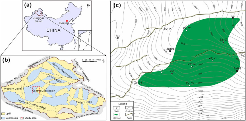
FIGURE 1. Regional tectonic position in the study area. (A) The location of the Junggar Basin. (B) The subdivisions of the Junggar Basin and the location of the Moxizhuang area. (C) The well locations in the Moxizhuang area. The green area shows the oil field.

Drilling data show that the second member (J₁s₂) of the Lower Jurassic Sangonghe Formation is mainly divided into upper and lower subsections according to their lithological characteristics, and the upper submember (J₁s₂^U) is mainly thick-layered mudstone with thin sandstone. The lower submember (J₁s₂^L) is mainly sandstone with some conglomerate. The Jurassic Sangonghe Formation in the Moxizhuang area has been carefully sedimentologically studied by previous researchers and is generally interpreted as a fluvial-deltaic sedimentary system (Zhang et al., 2000). In J₁s₂, with the contraction of the lake basin and strong hydrodynamic conditions, a large-scale sedimentary sand body with braided fluvial delta-meandering fluvial delta transitions is developed in the Moxizhuang area. J₁s₂^L is the frontal of the braided fluvial delta, with distributary sands that are very well developed, longitudinally superimposed sands and less mud deposition. J₁s₂^U is the frontal of the meandering fluvial delta, with an elevated water level and reduced material supply; the upper part has developed mudstone, and distributary channel sands and estuarine bar sands are deposited at the bottom (Cao et al., 2017; Wang et al., 2021).

The sandstone reservoir in J₁s₂ exhibits strong heterogeneous characteristics (see Figure 2), with effective reservoir rocks interacting via tight interlayers as transitions in the distributary channel, interchannel and estuary bar (see Figure 3). Controlled by sedimentary microfacies changes, the lithofacies in this member mainly consist of medium sandstone and fine sandstone, but mudstone and conglomerate are developed with relatively disparate proportions; additionally, there are large physical disparities between different lithofacies, with porosity mainly ranging from 2.0% to 20.0% (averaging 11.9%) and permeability mainly ranging from 0.01 to 500.0 mD (averaging 32.1 mD; these can be generally classified as dense reservoirs). According to its hydrocarbon shows, the sand distribution of a reservoir is discontinuous, whose tight interlayers act as the main barriers; the oil reservoirs have a complex oil-water distribution with frequent alternation of its oil, dry and water zones, which shows that the strong heterogeneity of the reservoir has a significant effect on the hydrocarbon accumulation.

FIGURE 2

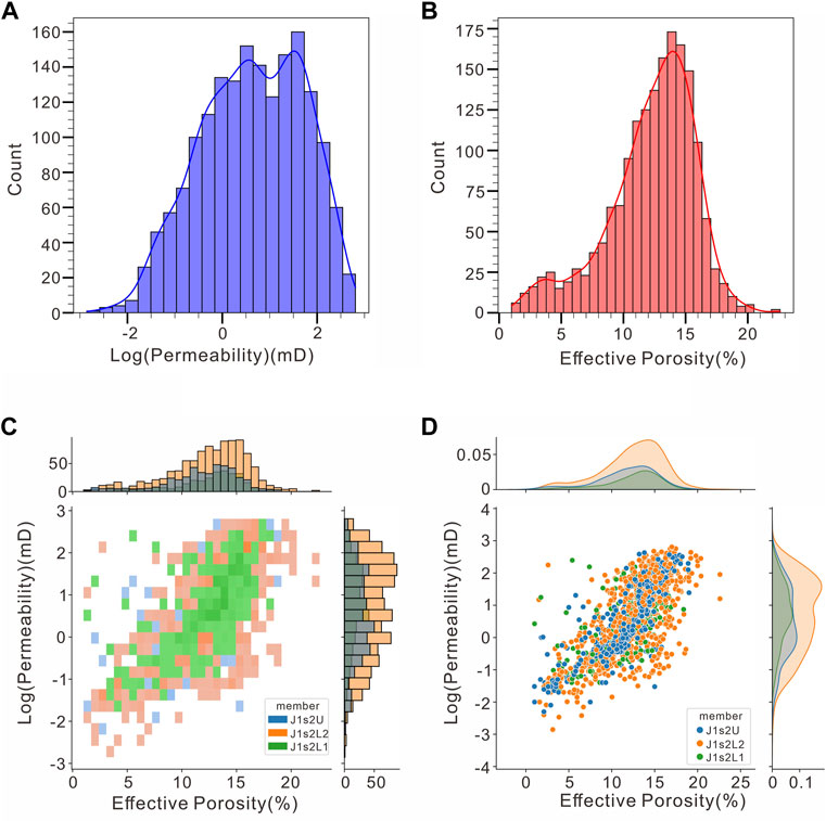
FIGURE 2. Porosity and permeability frequency histograms and joint probability distribution of the second section of t J₁s₂ in the Moxizhuang area. (A) Horizontal permeability frequency histogram. (B) Effective porosity frequency histogram. (C) Joint probability distribution of effective porosity and horizontal permeability (Different colors represent different members). (D) Cross-plot of effective porosity and horizontal permeability (Subplots are kernel density plots).

FIGURE 3

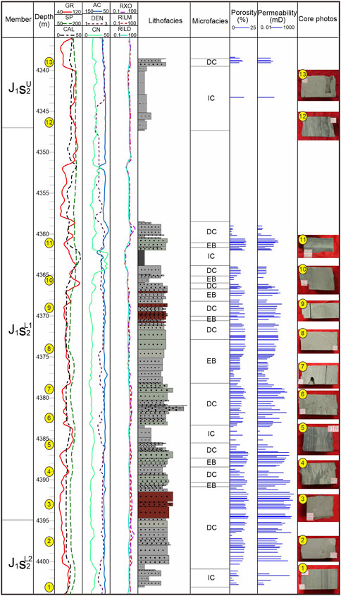
FIGURE 3. Single-well histogram of J₁s₂ in Well Zhuang 103 in the Moxizhuang area (IC in the sedimentary microfacies column represents the interchannel, DC represents the distributary channel, and EB represents the estuary bar).

3 Data and methods

3.1 Data

This study mainly considers the influences of grain size and composition on reservoir quality and classifies lithofacies from the perspective of the feasibility of logging identification based on core observations to provide geological labels for logging identification. According to the grain size standard (Krumbein, 1934; Miall, 1977), the overall grain size of the Sangonghe Formation reservoir is sandy, including very fine sand, fine sand, medium sand, and coarse sand, among which the medium- and fine-grained sandstone types are dominant; small amounts of gravel-bearing sandstone, muddy gravel sandstone, and conglomerate are also present, as shown in Table 1. The classification scheme helps when using logging for lithofacies identification without losing depositional characteristics. For the convenience of visualization, serial numbers are utilized instead of lithofacies.

TABLE 1

TABLE 1. Lithofacies classification comparison table for the Sangonghe Formation in the Moxizhuang area.

The core data categories of Zhuang 7, Zhuang 101, Zhuang 102, Zhuang 105, Zhuang 6, Zhuang 3 and Zheng 11 in the Moxizhuang area are complete, and the logging data of the target section are complete, so the data of these wells are mainly extracted for analysis purposes. Based on the sensitivity analysis and the completeness of the logging series, the nine conventional logging curves gamma ray (GR), spontaneous potential (SP), caliper (CAL), density (DEN), acoustic log(AC), compensated dual-spacing neutron (CN), Latero log 8 (RFOC), deep induction logging resistivity (RILD), and medium induction logging resistivity (RILM) are selected for lithologic classification.

In addition, different periods, logging series, environments and logging equipment can cause differences among logging data, and there is incomplete correspondence between the cores and logging depths due to the time lag of the coring. Therefore, preprocessing and core depth correction are required before processing logging data. In this study, we correct the core depth by the Depth shift function in Techlog and compare the GR curve to generate a depth shift table after stretching and panning the core profile.

3.2 Methodology

3.2.1 Naive Bayes

The Naive Bayesian approach is a supervised learning algorithm based on Bayesian theory, which assumes that the feature parameters are independent of each other (Zhang, 2004). Since the logging data are not strictly independent from each other, they cannot be easily used as direct input data for the classifier. Therefore, in this paper, the original logging data are subjected to singular value decomposition using the principal component analysis (PCA) method (Minka, 2000) and projected into a low-dimensional space with a linear transformation to obtain the uncorrelated variables X{$x_1,x_{2\cdots \cdots },x_n$}.

The mathematical expression of Bayesian theory is as follows:

$P\left(y|x_1,\dots ,x_n\right)=\frac{P\left(y\right)P\left(x_1,\dots x_n|y\right)}{P\left(x_1,\dots ,x_n\right)}(1)$

where $y$ is the category label; $x_1$…… $x_n$ represents the feature parameters; $P\left(y|x_1,\dots ,x_n\right)$ is the conditional probability of a set of observations corresponding to a specific category $y$, which is the posterior distribution; $P\left(y\right)$ is the prior probability of category $y$, which can be obtained from the core observations; and $P\left(x_1,\dots x_n|y\right)$ is the likelihood function.

Since the Naive Bayesian assumption states that the characteristic parameters are independent of each other, $P\left(x_1,\dots ,x_n\right)$ is a constant, and Eq. 1 is equivalent to:

$P\left(y|x_1,\dots ,x_n\right)\propto P\left(y\right){\displaystyle \prod }_{i=1}^{n}P\left(x_i|y\right)(2)$

where ${\displaystyle \prod }_{i=1}^{n}P\left(x_i|y\right)$ is the joint probability that the input variable is X conditional on the category $y$.

For each set of X, the category $\widehat{y}$ that maximizes $P\left(y|x_1,\dots ,x_n\right)$ is selected as the output category when making a decision:

$\widehat{y}={argmax}_{y}P\left(y\right){\displaystyle \prod }_{i=1}^{n}P\left(x_i|y\right)(3)$

From the principle of the Bayesian method, it is known that the key to the method is to obtain the appropriate prior $P\left(y\right)$ and likelihood function $P\left(x_i|y\right)$, which are usually obtained by using the maximum a posteriori probability (MAP) estimation and Markov chain Monte Carlo (MCMC) methods. However, Bayesian inference enables prior adjustment by applying Bayesian rules on different datasets (Dymarski, 2011), so the process can be independent of specific methods.

The assumptions of various likelihood functions differ, and their classifiers also differ. Since each lithofacies has input parameters characterized by a more obvious normal distribution, the Gaussian likelihood function is used in this paper to find the joint distribution. The formula for each characteristic is as follows:

$P\left(x_i|y_k\right)=\frac{1}{\sqrt{2\pi {\sigma }_{y_k,i}^2}}{e}^{-\frac{{\left(x_i-{\mu }_{y_k,i}\right)}^2}{2{\sigma }_{y_k,i}}}(4)$

where ${\mu }_{y_k,i}$ denotes the mean of feature $x_i$ in a sample with category $y_k$ and ${\sigma }_{y_k,i}^2$ denotes the variance of feature $x_i$ in a sample with category $y_k$. The parameters $\left.{\left[\mu \right.}_{y,1\dots n},{\sigma }_{y,1\dots n}^2\right]$ for each category $y$ can be estimated by the maximum likelihood method.

3.2.2 The Markov chain improves the prior probability

Modern geological studies have found that the iterative addition of deterministic relationships such as the rhythms, spirals, and cycles of rock formations and the stochastic relationships formed during deposition often give the resulting stratigraphic sequence a Markov chain property (Weissmann and Fogg, 1999; Elfeki and Dekking, 2001; Eidsvik et al., 2004). This Markov property is reflected in the lithofacies profile, which can provide an accurate estimation of the probability $P\left(y\right)$ of the distribution of different lithofacies within the reservoir inside the work area.

This property is expressed as follows: the conditional distribution for a future moment is only related to the current state if the present state is known, which is:

$\pi \left\{Y\left(t+1\right)=i_{n+1}|Y\left(t\right)=i_n,Y\left(t-1\right)=i_{n-1},Y\left(1\right)=i_1,Y\left(0\right)=i_0\right\}=\pi \left\{Y\left(t+1\right)=j|Y\left(t\right)=i\right\}(5)$

where $\pi$ is the probability, $Y\left(t\right)$ is the state at moment $t$ for the Markov chain, and $i,j$ is the value taken for its state. There is a linear correspondence between time and depth in a formation, so $Y\left(t\right)=Y\left(h\right)$ the above equation, which represents the state at position $h$ on the Markov chain.

Considering that a shallower formation depth corresponds to the later appearance of lithofacies, an upward Markov chain should be established for a single-well lithofacies sequence. Inferring the next position state needs to be realized by a transfer matrix, and the probability $P$ of transferring from state $i$ to $j$ is:

$P\left(i,j\right)=P\left(i\to j\right)=\pi \left\{Y_{t+1}=j\mid Y_t=i\right\}(6)$

The number of transitions in the whole classification process are calculated based on the core data from the bottom up and normalized to estimate the transfer probability so that the upward transfer probability matrix $P$ can be obtained. The random sequence transfer matrix $S$ is obtained according to the lithofacies proportions, and this matrix is used to determine the lower transfer probability of each type of lithofacies; then, the transfer matrix $P$ is modified.

After constructing the Markov transfer matrix $P$, an initial lithofacies distribution probability $\pi \left(0\right)$ is randomly given; then, the probabilities $\pi \left(t\right)=\pi \left(t-1\right)P=\dots =\pi \left(0\right)P^t$ are formed for different states at time $t$. After $n$ iterations over a long time period, $\pi \left(t\right)$ can be obtained for different iterative processes. When $n$ is sufficiently large, $\pi \left(t\right)$ becomes very close to the true lithofacies distribution, and thus the prior probability distribution is determined as:

$P\left(Y=j\right)=\underset{n\to \infty }{\mathit{lim}}{P\left(i,j\right)}^n={\displaystyle \prod }_{t=0}^{t=n}p\left({\pi }_{t+1}\mid {\pi }_t\right)\mid ={\pi }_j,j\in I(7)$

where $i$ and $j$ are lithofacies categories, $n$ is the number of iterations, the state space $I=\left\{0,1,2,\dots \right\}$ represents the total number of lithofacies categories, and ${\pi }_j$ is the probability of lithofacies $j$, which is approximated by iteration.

In addition, when calculating the prior probability $P\left(Y\right)$, it is necessary to consider how the Markov chain consisting of multiple wells calculates the transfer matrix, which should be weighted by depth to obtain the prior probability of the Moxizhuang area. Because the probability represented by $P\left(Y\right)$ is essentially not the frequency of the lithofacies distribution but rather the thickness of various lithofacies distributions in the case of stratigraphic determination, the former is strongly influenced by the sampling interval, and the latter is an inherent property of the formation. Compared with the conventional Bayesian method, the spatial relationships among the lithofacies distributions between different depth points (characterized by the transfer matrix) are considered in this a priori model, which is thus better constraining the spatio-temporal relationships of the sedimentary rocks.

3.2.3 Improving the likelihood function—Based on the synthetic minority oversampling technique and isotonic calibration

When performing parameter estimation for the likelihood function, the model will be biased because the likelihood function does not accurately describe the minority class distribution due to the effect of imbalance in the dataset, while the sample data of the minority class are not sufficiently characterized for the classifier to adequately learn them (Branco et al., 2016). One way to fight this issue is to generate new samples in underrepresented classes, which is also known as oversampling.

The oversampling method used in this paper is the K-means SMOTE (Chawla et al., 2002; Blagus and Lusa, 2013), which uses the K-means algorithm to cluster the input dataset classes and perform SMOTE within clusters with many minority class samples in safe and crucial areas of the input space, thus avoiding noise generation and effectively overcoming imbalances between and within classes (Douzas et al., 2018). K-means SMOTE consists of three steps: clustering, filtering and oversampling, as shown in Figure 4.

FIGURE 4

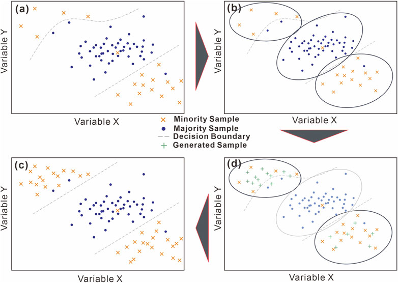
FIGURE 4. The K-means SMOTE oversamples safe areas and combats within-class imbalances (Douzas et al., 2018). (A) Input data. (B) Find k=3 clusters and compute the imbalance ratio (IR). (C) Use SMOTE to oversample clusters with IR>1, generating more samples in sparse clusters. (D). Oversampled data rectify the decision boundary.

In the clustering step, the input space is clustered into $k$ clusters using the K-means clustering method. $k$ is the most important hyperparameter in the K-means method, and finding the right value for k is crucial for the effectiveness of the K-means SMOTE, as it affects the number of minority class clusters found in the filtering step.

The filtering step selects the clusters to be oversampled and determines how many samples are to be generated in each cluster, with the aim of oversampling only the clusters where a few classes dominate while avoiding as much noise as possible and allocating the newly generated samples more to the sparse few-class clusters than to the dense clusters. This can be controlled with the imbalance ratio ($IR$) and sampling weights (${\alpha }_{os}$), as follows:

$IR=\frac{\mathit{majCount}\left(\mathit{c}\right)+\mathit{1}}{\mathit{minCount}\left(c\right)+1}(8)$

where $c$ is the clustering cluster label, $\mathrm{m}\mathrm{a}\mathrm{j}\mathrm{C}\mathrm{o}\mathrm{u}\mathrm{n}\mathrm{t}$ is the majority class sample count for that cluster, $\mathrm{m}\mathrm{i}\mathrm{n}\mathrm{C}\mathrm{o}\mathrm{u}\mathrm{n}\mathrm{t}$ is the minority class sample count for that cluster, and the imbalance ratio ($IR$) is the ratio of $\mathrm{m}\mathrm{a}\mathrm{j}\mathrm{C}\mathrm{o}\mathrm{u}\mathrm{n}\mathrm{t}$ to $\mathrm{m}\mathrm{i}\mathrm{n}\mathrm{C}\mathrm{o}\mathrm{u}\mathrm{n}\mathrm{t}$ for a particular cluster $c$.

${\alpha }_{os}=N_{rm}/N_M(9)$

where $N_{rm}$ is the number of samples in the minority class after resampling, $N_M$ is the number of samples in the majority class after resampling, and ${\alpha }_{os}$ corresponds to the ratio of $N_{rm}$ to $N_M$ after resampling. When performing multivariate classification, a distinction between the majority and minority class is needed.

In the oversampling step, SMOTE is applied in each selected cluster to boost the ratio ${\alpha }_{os}$ between the numbers of minority and majority samples. The SMOTE has the following flow. First, a random minority class observation $x_i$ is selected, and sample $x_{zi}$ is chosen among its k nearest minority class neighbors; a new sample is generated by the following equation:

$x_{new}=x_i+\lambda \times \left(x_{zi}-x_i\right)(10)$

where $\lambda$ is a random weight in (0, 1), and $x_i$ and $x_{zi}$ are the original samples of a minority class in the selected cluster.

In fact, applying oversampling methods may cause some other problems for the resulting model (Dal Pozzolo et al., 2015): variance increases (due to the change in sample size) and posterior distribution warping (due to the effect on the prior probabilities). The first problem can be solved by using averaging strategies to reduce the variance (Wallace et al., 2011), while the second problem requires the calibration of the new prior probabilities and updating the likelihood function. According to the Bayesian principle, the posterior probabilities obtained using partial sample inversions with guaranteed data independence can also be considered as the prior probabilities for reinversion. Therefore, this error can be corrected by calibrating the posterior probabilities of the initial inversion results.

The probabilistic calibration method not only uses the maximum posterior probability for discrimination but also includes a fitted regressor that maps the posterior probability of the classifier output to (0, 1) to obtain the calibration probability; that is, for a given sample of classifier output $f_i$, the calibrator predicts $p\left(y_i=1\mid f_i\right)$ (binary classification). For multiclass classification problems, the one-vs.-rest-classifier strategy is used to handle this, which involves fitting a classifier for each class, that is, fitted to all other classes (Zadrozny and Elkan, 2002). Isotonic regression is a commonly used probabilistic calibration method, that is, a nonparametric regression model approach, which considers that the function space is monotonically increasing (De Leeuw et al., 2010), so given a predicted probability $f_i$, the true probability is denoted as $y_i$:

$y_i=m\left(f_i\right)+{ϵ}_i(11)$

where $m$ denotes the monotonically increasing function, which is also the objective function to be fitted (Jiang et al., 2011), $ϵ$ is constants.

Then, the decision function is modified as follows:

$\widehat{y}={argmax}_{y}P\left(y\right)\times \widehat{m}\left({\displaystyle \prod }_{i=1}^{n}P\left(x_i|y\right)\right)(12)$

where the likelihood function is corrected using the isotonic function $\widehat{m}$:

$\widehat{m}={argmin}_w\sum {\left(y_i-w\left(f_i\right)\right)}^2(13)$

One algorithm that finds a stepwise constant solution for the Isotonic Regression problem is the pair-adjacent violators (PAV) algorithm (Ayer et al., 1955); the above equation can be simplified as:

$f\left(x\right)=minimize{\displaystyle \sum }_i{w}_i{\left(y_i-{\widehat{y}}_i\right)}^2,\mathit{s}\mathit{u}\mathit{b}\mathit{j}\mathit{e}\mathit{c}\mathit{t}\mathit{t}\mathit{o}{\widehat{y}}_i\le {\widehat{y}}_j\mathit{w}\mathit{h}\mathit{e}\mathit{n}\mathit{e}\mathit{v}\mathit{e}\mathit{r}{X}_i\le X_j(14)$

where the weights $w_i$ are strictly positive, the result should be a segmented linear function, and the modified likelihood function can be considered to reflect the distribution of the data features after oversampling.

3.2.4 Workflow

The flow of the whole method for lithofacies classification applications is shown in Figure 5. Through stepwise calibration and validation, the lithofacies information is propagated from the core section to the overburdened logging section, and the final lithofacies derived from different wells are geologically matched. This lithofacies parameter can be used for facies interpretation and reservoir modeling.

FIGURE 5

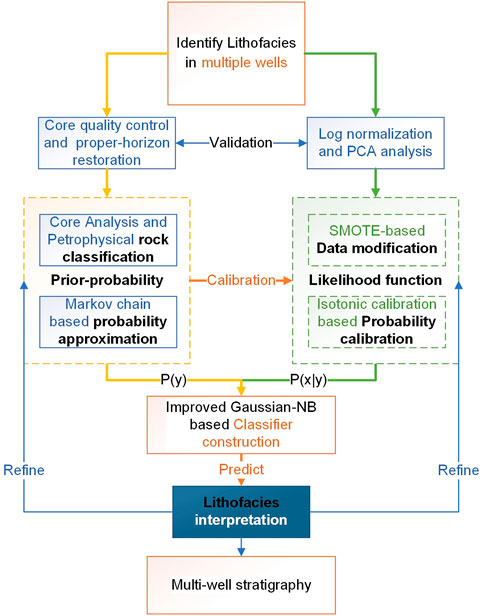
FIGURE 5. Lithofacies classification workflow based on well logs and core data.

3.3 Metrics

In this paper, a confusion (error) matrix (Powers, 2020) is used to evaluate the accuracy of classification. By definition, each column of the confusion (error) matrix represents the predicted category, and its total represents the data predicted to be in that category; each row represents the true attribution category of the data, and its total represents the number of instances in that category. The precision, recall and F1 score can be easily calculated on the basis of the confusion (error) matrix (Powers, 2020). K-fold cross-validation (Allen, 1974) was applied in the calculation to avoid underfitting and overfitting. The method distributes the training set into k smaller sets, and for each of the k “folded sets” the following process is performed: a single subsample is kept as validation data, and the rest of the samples are used for training, repeated the procession k times with each subsample validated once, resulting in a single estimate.

4 Results

4.1 Improving data imbalances

Due to the poor independence of the logging data, PCA conversion is needed, and oversampling is performed on this basis. In this study, the K-means SMOTE is utilized for processing, where the main parameters are IR and ${\alpha }_{os}$, the former controlling the algorithm that discriminates the imbalanced clusters, and the latter controlling the specific number of resampling operations per class. In addition, the clustering step uses the minibatch K-means algorithm, thus reducing the required computational time, and the size of the minibatch (which is a subset of the input data) is 1024. The oversampling step uses the nearest neighbors algorithm to determine the nearest neighbor samples, the number of neighbors set for the algorithm query is 5, and the neighbor distance is calculated by the Euclidean metric.

For the clustering step, the general number of clusters k should be similar to the actual number of categories, as shown in Figure 6. It appears that the clustering center tends to deviate from the clusters when setting k =8, so the number of clusters should be increased to make the clusters converge. Via continuous testing, we found that when the number of clusters was set to 56, the distribution interval of the clusters could be effectively characterized by the clustering center, and the sum of the squares of the distances from the samples to the nearest neighbors (inertia) was minimized.

FIGURE 6

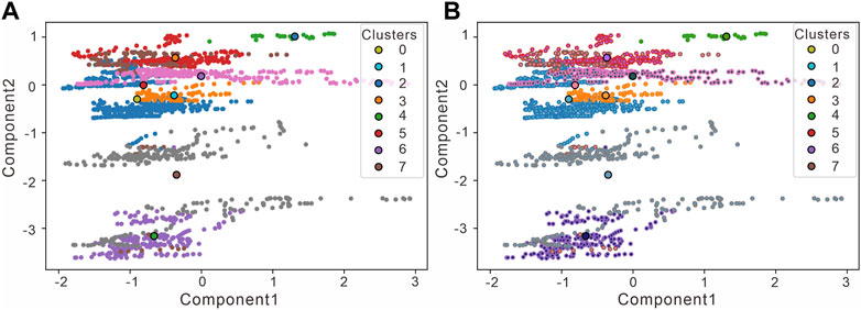
FIGURE 6. The clustering step is performed on the input data (PCA transformed). (A) The distance sum of squares (inertia) from the sample to the nearest neighbor is 6319.79 when setting K = 8, and the number of iterations is 12. (B) The distance sum of squares from the sample to the nearest neighbor is 891.84 when setting K = 56, and the number of iterations is 8.

For the sampling weight ${\alpha }_{os}$, since this is a multiclass study, the target class for resampling is specified as all classes except the majority class, and the ratio is set to guarantee that the numbers of samples in different classes are equal. For the imbalance ratio IR, the cluster selection process is more selective when the imbalance rate threshold is larger, and a higher proportion of minority samples is required to select clusters. However, the proportions of some minority class in this paper are too sparse (less than 5% of the total number of samples), and the common set threshold (generally 1) makes these classes fail to find suitable clusters for oversampling, so the criteria need to be relaxed. Therefore, in this paper, the threshold value is set to 0.25 based on continuous data characteristic testing to allow the selection of clusters with a high majority percentage. Clusters above this threshold are considered unbalanced and need to be oversampled. The number of samples for each lithofacies is determined based on the sampling weights [(0, 640), (1, 630), (2, 687), (4, 0), (3, 93), (5, 669), (6, 666), and (7, 710)].

Resampling was applied to the core data samples from the study area using the above-mentioned parameters and successfully enlarged the core data sample number from 2017 to 6128. The distribution of the newly generated sample is shown in Figure 7. Since the observed variables have high dimensionality, which is not conducive to observation, the feature variables are converted to two-dimensional variables by PCA, with the x-axis as principal component 1 and the y-axis as principal component 2; the cumulative variance contribution rate is 73%. Some of the feature spaces are not distributed with sample points, which may be related to the loss of variance, and principal components 1 and 2 cannot fully cover the variable space; it is also possible that the data points have limited characteristics or that comprehensive data are not collected.

FIGURE 7

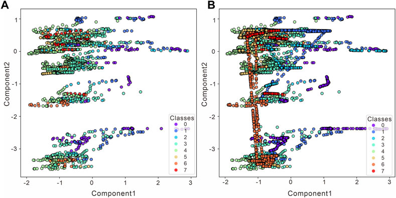
FIGURE 7. Changes in the lithofacies data distribution before and after K-means SMOTE (PCA transformed). (A) Origin data before resampling. (B) Resampling using K-mean SMOTE.

The left figure shows the distribution of the original dataset without conducting oversampling on two-dimensional variables, and the right figure shows the distribution of the data under two-dimensional variables after oversampling. The data distribution is more balanced after processing, while some discrete data points do not increase after filtering, such as 3 (fine sandstone) and 4 (medium sandstone). In addition, 7 (conglomerate) is the sparsest and fullest replenished. However, the data distribution is different from the original data distribution, and some points in the feature space are relatively densely distributed, thus affecting the prior probability when oversampling is performed. Additionally, the algorithm itself has distortion in the probability estimation, which requires probability calibration.

4.2 Introduction of geological priors

In this paper, the transfer matrix is calculated using the equally spaced stratigraphic unit method with a spacing of .125 m, which is consistent with the sampling interval of the logging curve. Based on the longitudinal distribution of the lithofacies obtained from the core observations, the label of each interval point is determined, and the depositional sequence is established after counting the lithofacies data of each well section in the Moxizhuang area; the specific processing flow is shown in Figure 8. In a single well, the numbers of transfers between different lithofacies are counted from bottom to top to form a single-well transfer matrix N. For the whole Moxizhuang area, the representative wells with continuous cores are selected as those with frequently changing lithofacies and complete information. The transfer matrices of these wells are summed up correspondingly according to the depth weighting to obtain the transfer matrix of the Moxizhuang area, forming the transfer matrix P shown in Table 2.

FIGURE 8

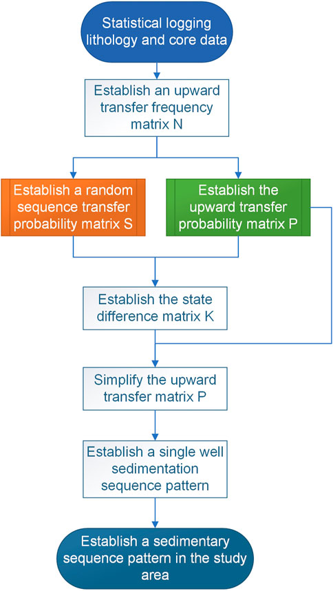
FIGURE 8. Sedimentation modeling process in the Moxizhuang area.

TABLE 2

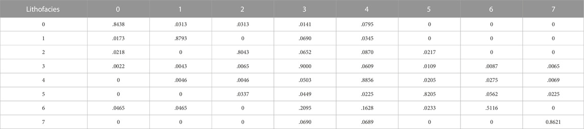
TABLE 2. Transfer matrix obtained from all core observations of the second section of the Sangonghe Formation in the Moxizhuang area.

The characteristics of the transfer matrix are briefly introduced by taking row 1 of the transfer matrix obtained from all core observations of Section 2 of the Sangonghe Formation in the Moxizhuang area in Table 2. In the core observations, lithofacies 5, 6 and 7 are not converted to lithofacies 0 located in the coarse-grained sandstone area (including coarse sandstone, gravel-bearing sandstone, and conglomerate). Above this depth, no mudstone can be developed directly from a sedimentary point of view. In contrast, lithofacies 1, 2, 3, and 4 can undergo conversion to 0 with probabilities of .0313, .0313, .0141, and .0795, respectively.

Based on the construction of the Markov transfer matrix, the average value of each lithofacies obtained statistically from the core observation is set as the initial probability, and the transfer matrix is used for iterative multiplication until a smooth distribution is obtained, which is the prior probability corresponding to the lithofacies distribution. Once the difference between the current matrix and the matrix of the previous iteration is less than the smooth error or the number of iterations reaches 100000, the matrix is accepted as a smooth distribution.

Figure 9 gives an example of the process of using a Markov chain to find the prior probabilities. The probabilities of different lithofacies in the figure tend to stabilize when the number of iterations reaches 80. It can be seen from the color phase diagram of the transfer matrix that the mudstone is relatively stable and not easily transformed into other lithofacies, while the gravel-bearing sandstone and muddy gravel sandstone are easily transformed into other lithofacies; this is also consistent with their geological significance. The mudstone is relatively stable in the sedimentary sequence and is structurally distinct from the other lithofacies, while the gravel-bearing sandstone and muddy gravel sandstone have wide ranges of grain sizes and are more compositionally distinct from the other lithofacies and therefore more easily converted.

FIGURE 9

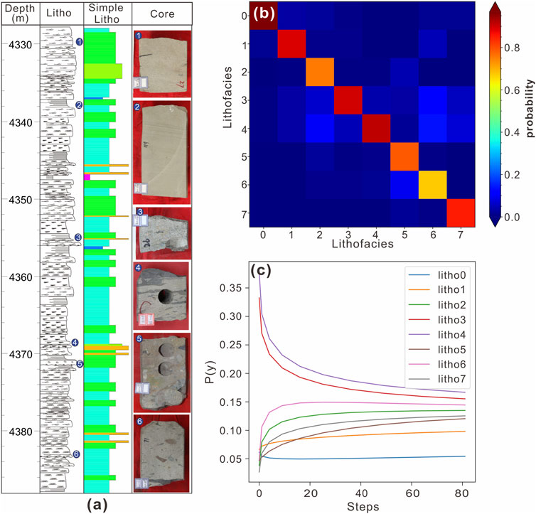
FIGURE 9. The iterative process of obtaining the prior probabilities. (A) The single-well deposition sequence (part of the Zhuang 101 well section is used as an example). Litho refers to lithofacies at the core scale. Simple Litho refers to lithofacies at the welling scale. (B) The color phase diagram of the transfer matrix. (C) The changes in the individual lithofacies probabilities during the iterative process.

The final calculation results show that the prior probability of the lithofacies is .095 (mudstone), .102 (very fine sandstone), .086 (muddy gravel sandstone), .211 (fine sandstone), .231 (medium sandstone), .101 (coarse sandstone), .173 (gravel-bearing sandstone), and 0.087 (conglomerate)). In other words, in Section II of the Sangonghe Formation, fine sandstone, medium sandstone and gravel-bearing sandstone have dominant positions and occur in the formation with a probability of approximately 20%, while other lithofacies are less, generally approximately 10%. To compare the effect of the a priori correction, the prior and likelihood are also calculated in this study according to the MCMC method, which is a common method for calculating such parameters in Bayesian methods, and the two parameters are found approximated together in this process. In fact, the prior probabilities are quite different from those obtained by the MCMC method, which are (.085, .101, .043, .291, .335, .058, .046, and .041), and the distribution probabilities of some lithofacies in the latter are relatively extreme and do not match well with the distribution of reservoir lithofacies in the Moxizhuang area.

4.3 Bayesian inversion and probability calibration

To perform Bayesian inversion, the prior is determined according to the Markov chain, and the likelihood is assumed to be Gaussian distributed, where the mean and variance are estimated according to the maximum likelihood method. The results are shown in Table 3.

TABLE 3

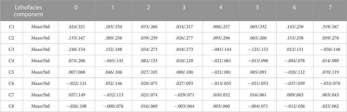
TABLE 3. Statistical table of the characteristic Gaussian parameter (Mean and Std) values for the input data corresponding to different lithofacies in the second section of the Sangonghe Formation in the Moxizhuang area.

Based on this, probability calibration is used to further improve the posterior distribution, and Figure 10 shows the difference between the probabilities predicted by the Naive Bayesian method for lithofacies 4, and the predicted probabilities optimized by two probability calibrations (isotonic regression and sigmoid function calibration) for different probability distribution phases and the true distribution probabilities (some points are shown). As seen from the figure, for different lithofacies, the probabilistic calibration method optimizes the predicted probabilities of the Naive Bayesian method on the basis of the likelihood function. This calibration is particularly evident in lithofacies 2, 3, 4, and 7, which also correspond to the lithofacies with the worst identification results for the Naive Bayesian method. The diagonal line in the figure indicates the case where the predicted probability is exactly the true probability. The orange line in the figure corresponds to the probability, that is, the predicted probability with isotonic regression calibration and thus the closest to the true sample probability. Because the isotonic regression process itself is directly optimized for the log loss, its own training process keeps the predicted probabilities as close to the true labels as possible.

FIGURE 10

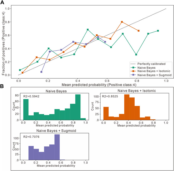
FIGURE 10. Comparison between Naive Bayesian identification and two probabilistic calibration curves for the second section of the Sangonghe Formation in the Moxizhuang area (taking fine sandstone as an example). (A) Calibration plots (reliability curve). It plots the true frequency of the positive label against its predicted probability, for binned predictions. (B) The histogram gives some insight into the behavior of each classifier by showing the number of samples in each predicted probability bin.

A set of improved Bayesian inversion processes is formed based on the above research, from which the confusion (error) matrix results are obtained by training in 7 wells in the work area. The outputs are compared with the original Naive Bayesian classification results, as shown in Figure 11. The left figure shows the results before improvement and the right figure shows the recognition results obtained after the improvement. Compared with that of the classifier before the improvement, the degree of confusion is greatly reduced, especially for classes 3, 4, 5 and 6. On the basis of the confusion (error) matrix, the precision, recall and F1 score values of the recognition results can be obtained, as shown in Table 4, and the recognition accuracy can reach approximately 0.84, which basically meets the requirements of lithofacies identification.

FIGURE 11

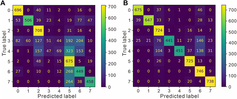
FIGURE 11. Comparison of the confusion (error) matrix before and after improvement. (A) The confusion (error) matrix of the Naive Bayes. (B) The confusion (error) matrix of the improved Bayes.

TABLE 4

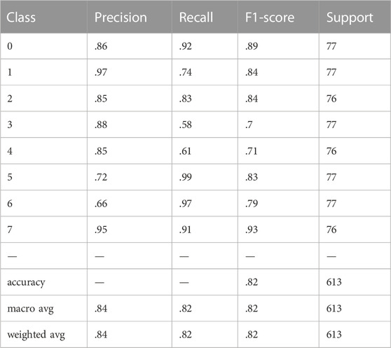
TABLE 4. Improved multiwell data identification results.

5 Discussion

5.1 Performance evaluation

To visually analyze the recognition effects of the Bayesian classifier before and after implementing the improvement described above, evaluate the bias and variance of the model, and test the generalizability of the proposed method, training is performed on 5 wells (Zhuang 7, Zhuang 101, Zhuang 102, Zhuang 105, and Zhuang 6) in the Moxizhuang area. Lithofacies prediction is performed on 2 wells (Zhuang 3 and Zheng 11), which did not participate in the inversion process; the characteristic variables are the conventional logging series.

In this study, learning curves are obtained using cross-validation (Figure 12 and Figure 13) to visualize whether the model is in an overfitted or underfitted state. The ideal learning curve should have a low bias and variance, representing convergence and low error. The horizontal axis of the left graph is the number of training samples, and the vertical axis represents the accuracy rate.

FIGURE 12

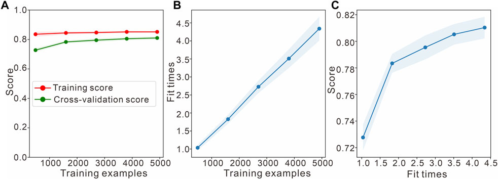
FIGURE 12. Learning curve of the Bayesian classifier for the inversion of J₁s₂. (A) Naive Bayes learning curves. (B) Scalability of the model. (C) Performance of the model. Fit times indicates the convergence time of the model training.

FIGURE 13

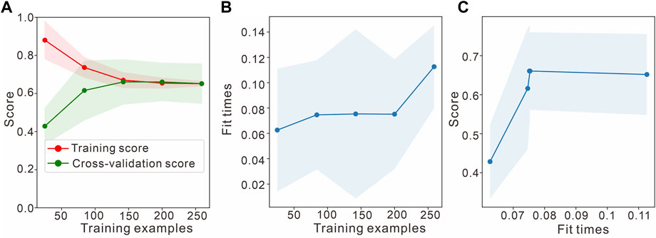
FIGURE 13. Learning curve of the improved Naive Bayesian classifier for the inversion of J₁s₂. (A) Learning curves of improved Bayes. (B) Scalability of the model. (C) Performance of the model.

Figure 12 shows that the accuracies of the Naive Bayesian method for the training and validation sets converge, but the accuracies after convergence are both approximately 0.62, which is much less than the desired accuracy; this can be considered an underfitting issue and requires increasing the complexity of the model, such as by adding features, increasing the number of classifiers, and reducing the interference terms. At this point, adding more data does not work. The middle figure shows the times required for the model to be trained using training datasets of various sizes; the model is relatively fast, which is consistent with the characteristics of Bayesian classifiers. Furthermore, it can be seen from the right figure that the correctness rate achieved in the test set increases slowly as the training time increases, corroborating the previous judgment. Figure 13 shows that the improved Bayesian classification method is able to solve this problem. It sacrifices some of the training time but meets the needs of the task in terms of accuracy. The study focuses on the application of the method to fluvial-delta environments, although its applicability is broader and it can be used to identify lithofacies in other depositional environments as well.

5.2 Fixed systematic errors caused by SMOTE

Oversampling methods can effectively expand the data size to reach the balance state, but most of them increase the samples based on local information. Although a relative equalization is achieved in terms of quantity, the data distribution of the new dataset obtained after oversampling cannot be guaranteed because the overall data distribution is not considered (Lv et al., 2018). In fact, the SMOTE algorithm may not overcome the data distribution problem, which tends to cause distribution marginalization. Since the distribution of a sample determines its optional neighbors, if a sample is located at the edge of the distribution of the sample set, the generated sample will also be located at that edge, thus blurring the boundary between different clusters. Although the fuzziness of the boundary improves the balance of the dataset, it also increases the difficulty of acquiring accurate prediction results (Li et al., 2021). This problem is difficult to characterize with a particular error, but it can be corrected with different methods depending on the impact of the SMOTE algorithm on the prior and likelihood.

For the prior probabilities, the SMOTE algorithm changes the distribution of the training samples of the data, so it is necessary to separate the calculation of the prior probabilities from the calculation of the likelihood function and adjust the prior function based on the presampling data only. Figure 14 shows the improved Bayesian probability spectrum for each lithofacies before and after introducing the prior. The introduction of the geological prior does not improve the single-point discrimination rate much, but the overall probability of each lithofacies distribution is obviously more consistent with the true values after its introduction; moreover, the transition of each lithofacies is not sharp, which yields better interpretation accuracy. And for single-point evaluation, the next step would be to improve the probabilistic calibration methods. The correct identification rate of a single point should be improved by correcting the expected probability of a certain class.

FIGURE 14

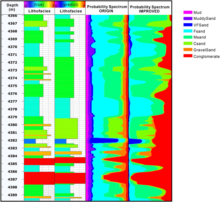
FIGURE 14. Comparison of core tagging probability spectra (taking the Chuang 105 well as an example). ORIGIN means no sampling was performed and the prior and likelihood were calculated using the MCMC method. IMPROCVED represents that Markov chains were used to calculate a priori posterior and to improve data imbalance using the SMOTE method.

In addition, the problem of sample overlap can lead to anomalies in the parameters of the likelihood function and thus the posterior distribution. In contrast, the probability calibration method used in this paper can recalculate the likelihood using the initial inversion results as the prior to improve the probability distribution. Figure 15 shows the changes in the discrimination probabilities of fine and medium sandstone before and after performing probability calibration, with approximately 10% real samples and 90% confused samples. The horizontal axis is sorted according to the predicted probabilities, which shows that the classifier can discriminate the confused samples more accurately after calibration. In fact, the accuracies achieved for all types are higher after the improvement, and those of fine sandstone, medium sandstone, coarse sandstone and gravel-bearing sandstone, which cannot be better identified through the original Bayesian inversion process, are also improved.

FIGURE 15

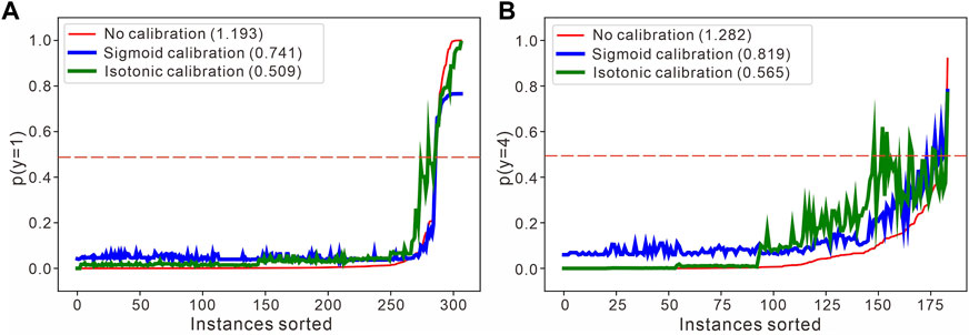
FIGURE 15. Specific discriminatory adjustment of the two-segment probability calibration curve of the Sangonghe Formation. (A)The very fine-grained sandstone probability is taken as an example. (B) The medium-grained sandstone probability is taken as an example. The input samples are sorted according to the discriminatory recognition results as the category probabilities, and the number in the upper left corner of the figure represents the log loss.

6 Conclusion

Lithofacies identification in deep strongly heterogeneous reservoirs is a complex nonlinear classification problem. In this study, we explore solutions to the key problems faced during the process of lithofacies identification when using machine learning methods by taking conventional logging data from the second member of the Sangonghe Formation in the Moxizhuang area as an example, and establish a set of Bayesian inversion prediction processes that are applicable to the lithofacies of strongly heterogeneous reservoirs, taking core data as a constraint. The following conclusions are mainly obtained.

1) Frequent lithofacies changes in deep strongly heterogeneous reservoirs pose a challenge to the traditional point-by-point machine learning-based identification method. The depositional prior construction technique based on Markov chains can better constrain the depositional spreading process of the vertical lithofacies so that the predicted vertical distribution of the lithofacies conforms to geological constraints.

2) Strongly heterogeneous reservoirs exhibit relatively disparate lithofacies proportions, forming a data imbalance problem that causes logging data to fail to fully reflect the characteristics of minority categories. The likelihood function correction method that uses the K-means SMOTE with probabilistic calibration can solve the data imbalance problem of lithofacies identification in strongly heterogeneous reservoirs.

3) A set of improved Bayesian lithofacies evolution process is established and applied to lithofacies identification and prediction for multiple wells in the Moxizhuang area. An application of this approach to the fluvial-deltaic reservoirs of the Sangonghe Formation in the Moxizhuang area shows that the new method improves the recognition accuracy by 20% over that of the traditional machine learning method and can more accurately identify the lithofacies types of deep strongly heterogeneous reservoirs.

The method proposed in this paper can realize pattern recognition for lithofacies logging, but subsequent work is needed to improve the accuracy by using the internal hierarchies of lithofacies, introducing the idea of sedimentation prior into other related algorithms to improve them, and further matching with the automatic logging stratification method to realize modular data recognition. The method can identify the lithofacies for deep and strongly inhomogeneous clastic reservoirs, and provide a reference for future exploration and development.

Data availability statement

The raw data supporting the conclusion of this article will be made available by the authors, without undue reservation.

Author contributions

ZoZ was responsible for the overall programming and writing of the article. LZ was responsible for the correction of the article and the guidance of the overall idea. MC was responsible for the guidance of the machine learning part. YL provided guidance. Other authors gave help with figure revisions and data provision.

Funding

This study is supported by the National Natural Science Foundation of China (42030808, 42102176), and the Strategic Priority Research Program of the Chinese Academy of Sciences (XDA14010202).

Acknowledgments

The study would not have been possible without the support from Sinopec Shengli Oil Company, we thank Shengli Oil Company for permission to publish this work. Acocella V. and several anonymous reviewers are appreciated for their critical comments and insightful suggestions, which significantly improve the quality of this article.

Conflict of interest

The authors ZeZ, ZhZ, and XR were employed by the company Sinopec Shengli Oilfield Company. The author LY was employed by Sinopec Petroleum Exploration and Production Research Institute. The author WY was employed by AspenTech Subsurface Science and Engineering.

The remaining authors declare that the research was conducted in the absence of any commercial or financial relationships that could be construed as a potential conflict of interest.

Publisher’s note

All claims expressed in this article are solely those of the authors and do not necessarily represent those of their affiliated organizations, or those of the publisher, the editors and the reviewers. Any product that may be evaluated in this article, or claim that may be made by its manufacturer, is not guaranteed or endorsed by the publisher.

References

Al-Mudhafar, W. J., Abbas, M. A., and Wood, D. A. (2022). Performance evaluation of boosting machine learning algorithms for lithofacies classification in heterogeneous carbonate reservoirs. Mar. Petroleum Geol. 145, 105886. doi:10.1016/j.marpetgeo.2022.105886

CrossRef Full Text | Google Scholar

Allen, D. M. (1974). The relationship between variable selection and data agumentation and a method for prediction. technometrics 16 (1), 125–127. doi:10.1080/00401706.1974.10489157

CrossRef Full Text | Google Scholar

Antariksa, G., Muammar, R., and Lee, J. (2022). Performance evaluation of machine learning-based classification with rock-physics analysis of geological lithofacies in Tarakan Basin, Indonesia. J. Petroleum Sci. Eng. 208, 109250. doi:10.1016/j.petrol.2021.109250

CrossRef Full Text | Google Scholar

Asfahani, J. (2014). Statistical factor analysis technique for characterizing basalt through interpreting nuclear and electrical well logging data (case study from Southern Syria). Appl. Radiat. Isotopes 84, 33–39. doi:10.1016/j.apradiso.2013.09.019

PubMed Abstract | CrossRef Full Text | Google Scholar

Ayer, M., Brunk, H. D., Ewing, G. M., Reid, W. T., and Silverman, E. (1955). An empirical distribution function for sampling with incomplete information. Ann. Math. statistics 26, 641–647. doi:10.1214/aoms/1177728423

CrossRef Full Text | Google Scholar

Blagus, R., and Lusa, L. (2013). SMOTE for high-dimensional class-imbalanced data. BMC Bioinforma. 14 (1), 106. doi:10.1186/1471-2105-14-106

PubMed Abstract | CrossRef Full Text | Google Scholar

Bloch, S., Lander, R. H., and Bonnell, L. (2002). Anomalously high porosity and permeability in deeply buried sandstone reservoirs: Origin and predictability. AAPG Bull. 86 (2), 301–328. doi:10.1306/61eedabc-173e-11d7-8645000102c1865d

CrossRef Full Text | Google Scholar

Branco, P., Torgo, L., and Ribeiro, R. P. (2016). A Survey of predictive modeling on imbalanced domains. ACM Comput. Surv. 49 (2), 1–50. Article 31. doi:10.1145/2907070

CrossRef Full Text | Google Scholar

Cao, B., Luo, X., Zhang, L., Sui, F., Lin, H., and Lei, Y. (2017). Diagenetic evolution of deep sandstones and multiple-stage oil entrapment: A case study from the lower jurassic Sangonghe Formation in the fukang sag, central Junggar Basin (NW China). J. Petroleum Sci. Eng. 152, 136–155. doi:10.1016/j.petrol.2017.02.019

CrossRef Full Text | Google Scholar

Chawla, N. V., Bowyer, K. W., Hall, L. O., and Kegelmeyer, W. P. (2002). Smote: Synthetic minority over-sampling technique. J. Artif. Intell. Res. 16, 321–357. doi:10.1613/jair.953

CrossRef Full Text | Google Scholar

Chen, C., and Hiscott, R. N. (1999). Statistical analysis of turbidite cycles in submarine fan successions; tests for short-term persistence. J. Sediment. Res. 69 (2), 486–504. doi:10.2110/jsr.69.486

CrossRef Full Text | Google Scholar

Chen, F., Wang, X., and Wang, X. (2005). Prototype and tectonic evolution of the Junggar Basin, northwestern China. Earth Sci. Front. 12 (3), 77. doi:10.3321/j.issn:1005-2321.2005.03.010

CrossRef Full Text | Google Scholar

Dal Pozzolo, A., Caelen, O., and Bontempi, G. (2015). “When is undersampling effective in unbalanced classification tasks?,” in Joint european conference on machine learning and knowledge discovery in databases.

CrossRef Full Text | Google Scholar

De Leeuw, J., Hornik, K., and Mair, P. (2010). Isotone optimization in R: Pool-adjacent-violators algorithm (PAVA) and active set methods. J. Stat. Softw. 32, 1–24. doi:10.18637/jss.v032.i05

CrossRef Full Text | Google Scholar

Douzas, G., Bacao, F., and Last, F. (2018). Improving imbalanced learning through a heuristic oversampling method based on k-means and SMOTE. Inf. Sci. 465, 1–20. doi:10.1016/j.ins.2018.06.056

CrossRef Full Text | Google Scholar

Dunham, M. W., Malcolm, A., and Welford, J. K. (2020). Improved well log classification using semisupervised Gaussian mixture models and a new hyper-parameter selection strategy. Comput. Geosciences 140, 104501. doi:10.1016/j.cageo.2020.104501

CrossRef Full Text | Google Scholar

Dymarski, P. (2011). Hidden Markov models: Theory and applications. Hamburg, Germany: BoD–Books on Demand.

Google Scholar

Eidsvik, J., Mukerji, T., and Switzer, P. (2004). Estimation of geological attributes from a well log: An application of hidden Markov chains. Math. Geol. 36 (3), 379–397. doi:10.1023/b:matg.0000028443.75501.d9

CrossRef Full Text | Google Scholar

Elfeki, A., and Dekking, M. (2001). A Markov chain model for subsurface characterization: Theory and applications. Math. Geol. 33 (5), 569–589. doi:10.1023/a:1011044812133

CrossRef Full Text | Google Scholar

Feng, R., Luthi, S. M., Gisolf, D., and Angerer, E. (2018). Reservoir lithology classification based on seismic inversion results by Hidden Markov Models: Applying prior geological information. Mar. Petroleum Geol. 93, 218–229. doi:10.1016/j.marpetgeo.2018.03.004

CrossRef Full Text | Google Scholar

Feng, R. (2021). Uncertainty analysis in well log classification by Bayesian long short-term memory networks. J. Petroleum Sci. Eng. 205, 108816. doi:10.1016/j.petrol.2021.108816

CrossRef Full Text | Google Scholar

Gu, Y., Bao, Z., Song, X., Patil, S., and Ling, K. (2019). Complex lithology prediction using probabilistic neural network improved by continuous restricted Boltzmann machine and particle swarm optimization. J. Petroleum Sci. Eng. 179, 966–978. doi:10.1016/j.petrol.2019.05.032

CrossRef Full Text | Google Scholar

Gu, Y., Zhang, D., Lin, Y., Ruan, J., and Bao, Z. (2021). Data-driven lithology prediction for tight sandstone reservoirs based on new ensemble learning of conventional logs: A demonstration of a yanchang member, ordos basin. J. Petroleum Sci. Eng. 207, 109292. doi:10.1016/j.petrol.2021.109292

CrossRef Full Text | Google Scholar

Hammer, H., Kolbjørnsen, O., Tjelmeland, H., and Buland, A. (2012). Lithology and fluid prediction from prestack seismic data using a Bayesian model with Markov process prior. Geophys. Prospect. 60 (3), 500–515. doi:10.1111/j.1365-2478.2011.01012.x

CrossRef Full Text | Google Scholar

He, H., and Garcia, E. A. (2009). Learning from imbalanced data. IEEE Trans. Knowl. data Eng. 21 (9), 1263–1284. doi:10.1109/tkde.2008.239

CrossRef Full Text | Google Scholar

Hu, C., and Sun, B. (2020). “Multitask learning for petrophysical attribute prediction using convolutional neural network and imbalance dataset,” in Proceeding of the SEG International Exposition and Annual Meeting, Virtual, October 2020.

CrossRef Full Text | Google Scholar

Jiang, X., Osl, M., Kim, J., and Ohno-Machado, L. (2011). Smooth isotonic regression: A new method to calibrate predictive models. AMIA Summits Transl. Sci. Proc. 2011, 16.

PubMed Abstract | Google Scholar

Kim, D., and Byun, J. (2020). “Data augmentation using CycleGAN for overcoming the imbalance problem in petrophysical facies classification,” in SEG technical Program expanded abstracts 2020, 2310–2314. doi:10.1190/segam2020-3427510.1

CrossRef Full Text | Google Scholar

Kjønsberg, H., Hauge, R., Kolbjørnsen, O., and Buland, A. (2010). Bayesian Monte Carlo method for seismic predrill prospect assessment. Geophysics 75 (2), O9–O19. doi:10.1190/1.3339678

CrossRef Full Text | Google Scholar

Krumbein, W. C. (1934). Size frequency distributions of sediments. J. Sediment. Res. 4 (2), 65–77. doi:10.1306/d4268eb9-2b26-11d7-8648000102c1865d

CrossRef Full Text | Google Scholar

Lai, J., Fan, X., Liu, B., Pang, X., Zhu, S., Xie, W., et al. (2020). Qualitative and quantitative prediction of diagenetic facies via well logs. Mar. Petroleum Geol. 120, 104486. doi:10.1016/j.marpetgeo.2020.104486

CrossRef Full Text | Google Scholar

Larsen, A. L., Ulvmoen, M., Omre, H., and Buland, A. (2006). Bayesian lithology/fluid prediction and simulation on the basis of a Markov-chain prior model. Geophysics 71 (5), R69–R78. doi:10.1190/1.2245469

CrossRef Full Text | Google Scholar

Li, D. Z., Liu, J. X., and Liu, J. (2021). NNI-SMOTE-XGBoost: A novel small sample analysis method for properties prediction of polymer materials. Macromol. Theory Simulations 30 (5), 2100010. ARTN 2100010. doi:10.1002/mats.202100010

CrossRef Full Text | Google Scholar

Li, Z., Zhang, L., Yuan, W., Chen, X., Zhang, L., and Li, M. (2022). Logging identification for diagenetic facies of tight sandstone reservoirs: A case study in the lower jurassic ahe formation, kuqa depression of tarim basin. Mar. Petroleum Geol. 139, 105601. doi:10.1016/j.marpetgeo.2022.105601

CrossRef Full Text | Google Scholar

Liu, J. J., and Liu, J. C. (2022). Integrating deep learning and logging data analytics for lithofacies classification and 3D modeling of tight sandstone reservoirs. Geosci. Front. 13 (1), 101311. doi:10.1016/j.gsf.2021.101311

CrossRef Full Text | Google Scholar

Liu, J., Liu, Z., Xiao, K., Huang, Y., and Jin, W. (2020). Characterization of favorable lithofacies in tight sandstone reservoirs and its significance for gas exploration and exploitation: A case study of the 2nd member of triassic xujiahe Formation in the xinchang area, sichuan basin. Petroleum Explor. Dev. 47 (6), 1194–1205. doi:10.1016/S1876-3804(20)60129-5

CrossRef Full Text | Google Scholar

Lv, D., Ma, Z., Yang, S., Li, X., Ma, Z., and Jiang, F. (2018). The application of SMOTE algorithm for unbalanced data. Proceedings of the 2018 International Conference on Artificial Intelligence and Virtual Reality. November 2018. 10–13.

CrossRef Full Text | Google Scholar

Miall, A. D. (1977). Lithofacies types and vertical profile models in braided river deposits: A summary.

Google Scholar

Minka, T. (2000). “Automatic choice of dimensionality for PCA,” in Advances in neural information processing systems, 13.

Google Scholar

Powers, D. M. (2020). Evaluation: From precision, recall and F-measure to ROC, informedness, markedness and correlation. arXiv [Preprint] 2010, 16061. Available at: https://arxiv.org/abs/2010.16061.

Google Scholar

Press, W., Teukolsky, S., Vetterling, W., and Flannery, B. (2007). “Gaussian mixture models and k-means clustering,” in Numerical recipes. The art of scientific computing, 3rd ed. (Cambridge University Press), 843–846.

Google Scholar

Qin, R., Pan, H., Zhao, P., Deng, C., Peng, L., Liu, Y., et al. (2018). Petrophysical parameters prediction and uncertainty analysis in tight sandstone reservoirs using Bayesian inversion method. J. Nat. Gas Sci. Eng. 55, 431–443. doi:10.1016/j.jngse.2018.04.031

CrossRef Full Text | Google Scholar

Ren, Q., zhang, H., Zhang, D., Zhao, X., Yan, L., and Rui, J. (2022). A novel hybrid method of lithology identification based on k-means++ algorithm and fuzzy decision tree. J. Petroleum Sci. Eng. 208, 109681. doi:10.1016/j.petrol.2021.109681

CrossRef Full Text | Google Scholar

Song, S., Hou, J., Dou, L., Song, Z., and Sun, S. (2020). Geologist-level wireline log shape identification with recurrent neural networks. Comput. Geosciences 134, 104313. doi:10.1016/j.cageo.2019.104313

CrossRef Full Text | Google Scholar

Su, F., Ma, L., Luo, R.-z., and Ni, Y. (2020). Research and application of logging lithology identification based on improve multi-class twin support vector machine. Prog. Geophys. 35 (1), 174–180. doi:10.1016/j.jappgeo.2019.103929

CrossRef Full Text | Google Scholar

Thomas, E., Ec, T., and Ra, H. (1977). Log derived shale distribution in sandstone and its effect upon porosity, water saturation and permeability.

Google Scholar

Wallace, B. C., Small, K., Brodley, C. E., and Trikalinos, T. A. (2011). Class imbalance, redux. Proceeding of the 2011 IEEE 11th international conference on data mining. December 2011. IEEE. Vancouver, BC, Canada.

CrossRef Full Text | Google Scholar

Wang, J., Xu, S., Ren, X., Chi, X., Shu, P., Liu, X., et al. (2021). Diageneses and controlling factors of Jurassic Sangonghe Formation reservoirs on the west side of the hinterland of Junggar Basin. Acta Pet. Sin. 42 (3), 319–331. Available at: http://www.syxb-cps.com.cn. doi:10.7623/syxb202103005

CrossRef Full Text | Google Scholar

Weissmann, G. S., and Fogg, G. E. (1999). Multi-scale alluvial fan heterogeneity modeled with transition probability geostatistics in a sequence stratigraphic framework. J. Hydrology 226 (1), 48–65. doi:10.1016/S0022-1694(99)00160-2

CrossRef Full Text | Google Scholar

Xu, C. (2013). Reservoir description with well-log-based and core-calibrated petrophysical rock classification. Austin, TX, United States: The University of Texas at Austin.

Google Scholar

Zadrozny, B., and Elkan, C. (2002). Transforming classifier scores into accurate multiclass probability estimates Proceedings of the eighth ACM SIGKDD international conference on Knowledge discovery and data mining, January 2002, Edmonton, Alberta, Canada. doi:10.1145/775047.775151

CrossRef Full Text | Google Scholar

Zhang, H., Dessimoz, J., Beyer, T. A., Krampert, M., Williams, L. T., Werner, S., et al. (2004). Fibroblast growth factor receptor 1-IIIb is dispensable for skin morphogenesis and wound healing. AA 1 (2), 3–11. doi:10.1078/0171-9335-00355

PubMed Abstract | CrossRef Full Text | Google Scholar

Zhang, M., Zhu, X., and Zhang, Q. (2000). Jurassic sedimentary system of east Junggar Basin and its hydrocarbon significance. Oil Gas. Geol. 21 (3), 272–278. doi:10.3321/j.issn:0253-9985.2000.03.019

CrossRef Full Text | Google Scholar

Zhang, L. K., Luo, X. R., Ye, M. Z., Zhang, B. S., Wei, H. X., Cao, B. F., et al. (2021). Small-scale diagenetic heterogeneity effects on reservoir quality of deep sandstones: A case study from the lower jurassic ahe formation, eastern kuqa depression. Geofluids 2021, 1–25. doi:10.1155/2021/6626652

CrossRef Full Text | Google Scholar

Zheng, D., Hou, M., Chen, A., Zhong, H., Qi, Z., Ren, Q., et al. (2022). Application of machine learning in the identification of fluvial-lacustrine lithofacies from well logs: A case study from sichuan basin, China. J. Petroleum Sci. Eng. 215, 110610. doi:10.1016/j.petrol.2022.110610

CrossRef Full Text | Google Scholar

Zhou, Z., Wang, G., Ran, Y., Lai, J., Cui, Y., and Zhao, X. (2016). A logging identification method of tight oil reservoir lithology and lithofacies: A case from Chang7 member of triassic yanchang Formation in heshui area, ordos basin, NW China. Petroleum Explor. Dev. 43 (1), 65–73. doi:10.1016/S1876-3804(16)30007-6

CrossRef Full Text | Google Scholar

Zhou, K., Zhang, J., Ren, Y., Huang, Z., and Zhao, L. (2020). A gradient boosting decision tree algorithm combining synthetic minority oversampling technique for lithology identification. Geophysics 85 (4), WA147–WA158. doi:10.1190/geo2019-0429.1

CrossRef Full Text | Google Scholar