 Lingling Liu
 Gang Cheng
 Jie Yang1
- 1School of Surveying and Land Information Engineering, Henan Polytechnic University, Jiaozuo, China
- 2Mineral Resources Exploration Center of Henan Geological Bureau, Zhengzhou, China
Fine-scale population map plays an essential role in numerous fields, including resource allocation, urban planning, disaster prevention and response. Point of Interest (POI) data is widely used for population spatialization, but the types of POI are ignored. Since different types of POI data have different impacts on population distribution, this paper used typed POI data and other multi-source data to map population distributions at fine scales. At the township level, three random forest models were used to generate the population maps of 150 m, 300 m, and 500 m in 2020, enabling the downscaling of county-level population distribution to the grid level. The main influencing factors of population distribution were extracted and analyzed based on the feature importance output from the model. Zhengzhou city was used as a case for study. The experiments show the results of population spatialization for all three scales in this study have better fitting accuracy than that of the GPWv4 and LandScan datasets. The coefficient of determination (
1 Introduction
Demographic data reveal entire population counts in entire administrative units, ignoring the detailed characteristics of population distribution within the units (Wang et al., 2018; Xiong et al., 2019), making it difficult to accurately understand the actual population distribution within an administrative unit or across administrative units. Meanwhile, the demand for high-resolution population distribution data is growing. Population spatialization is to use demographic data, administrative boundaries, and suitable ancillary data to dis-aggregate demographic data in administrative districts to regular grids of a certain size through certain modeling methods (Bai et al., 2013; Dong et al., 2016), so as to present information on the spatial distribution of population. Fine grid population distribution can reproduce the population geographic distribution of the objective world, solve the problem of disconnection between population statistics and the spatial characteristics of the regions they belong to (Fu et al., 2014), and provide basic data support for the coupling analysis of population data with natural resources and socio-economic data. Fine-scale population distribution also helps to solve the problems of urban planning, resource allocation, disaster prevention and response, public health, etc (Li et al., 2018; Wang et al., 2020).
With the development of remote sensing and Geographic Information System (GIS) technology, the supporting methods and data of population spatialization are constantly changing and enriching. In terms of population simulation methods, population density models (Clark, 1951; Jiang et al., 2002) and spatial interpolation methods (Martin, 1996; Mennis, 2003) were used in the early days, which evolved to the use of statistical regression models, including geographically weighted regression (GWR), spatial regression models (Spatial Lag Model, SLM and Spatial Error Model, SEM), and multiple linear regression (MLR) (Lo, 2008; Chun et al., 2018; Yang and Chen, 2019), and gradually evolved to the application of machine learning models (He et al., 2020; Li and Liu, 2021) and deep learning models (Zhao et al., 2020; Cheng et al., 2021). Most of the early population spatialization research is based on a certain kind of data, and now it has developed into the fusion of multi-source geospatial data. Based on the assumption that the same land type carries the same population density (Bai et al., 2013; Bakillah et al., 2014; Dong et al., 2016), Land use/cover data are the most widely used data in population spatialization. In fact, due to many factors affecting population distribution, the assumption is not always correct. Nighttime light can reflect socioeconomic activities and human activities and has a strong correlation with residential areas (Guo et al., 2021). However, there is always low accuracy and underperformance in areas with low brightness when using nighttime light data alone for population spatialization (Xiao and Yang, 2019). Therefore, land cover/use data and nighttime light data are often used together in population spatialization studies (Briggs et al., 2007; Zeng et al., 2011; Hu et al., 2018; Xiong et al., 2019), to make up for the shortage of single data. There are many publicly available nighttime light data, such as DMSP/OLS, NPP/VIIRS, and Luojia1-01 data, among which Luojia1-01 data has the highest spatial resolution (approximately 130 m) (Ou et al., 2019), which is more favorable for fine-scale population fitting (Zou et al., 2020; Sun et al., 2021; Wang and Zhang, 2021).
In the era of big data, with the rapid development and availability of social sensing data (e.g., check-in data on social media, POI data, mobile phone data, etc.), new opportunities have become available for examining fine-scale populations. POI data is a kind of big data generated with Internet maps, such as Baidu Map, AutoNavi Map, and OpenStreetMap (OSM), and can be easily obtained through Application Programming Interface (API) (Zhang et al., 2021). POI data includes information on almost all kinds of facilities and places closely related to the production and life of urban residents and is characterized by large quantity, easy access, fast update, and rich information (Yao et al., 2017; Sun et al., 2021; Zeng et al., 2021). Many scholars have used POI data to map population distribution. Chun et al. (2018) who proposed a method for gridding population distribution based on POI data using quadtree spatial indexing. Zou et al. (2020) who proposed a method to fuse nighttime light and POI data by multiplying POI kernel density data with Luojia1-01 nighttime light data processed by logarithmic transformation, and then normalizing the result to 0∼255 after squaring, which provides a new method for processing population spatialization data. Ye et al. (2019) who weighted the 20 types of POI density layers to combine into one density layer and calculated the distance to the nearest POI to obtain a raster layer in the same way, and then two raster layers were involved in modeling. POI data can represent lots of geographic entities with various types, such as schools, hospitals, restaurants, shopping malls, transportation facilities, and enterprises. Different types of POI represent different human activities within and surrounding them, and subsequently have different levels of correlation with population distribution (Bakillah et al., 2014; Ye et al., 2019). For example, living facilities often appear around residential areas. The more they are, the denser the local population is. However, the impact of different types of POIs on the population simulation has not been paid enough attention to and is often even ignored. Thereby, further research is needed to study how to use typed POI data to obtain a fine-grained population distribution.
In this paper, typed POI data coupled with Luojia1-01 nighttime light data, land cover data, DEM data, and road network data were used to get fine-scale population distributions, and Zhengzhou city was set as a case study. Three random forest models were established to generate the population maps with spatial resolutions of 150 m, 300 m, and 500 m in 2020, respectively. The types of POIs with significant roles were extracted and analyzed by feature importance. In addition, the role of typed POIs in population spatialization was further illustrated by comparing the precision and population maps of the three sets of experiments conducted around POIs.
2 Materials and methods
2.1 Study area
Zhengzhou, the capital city of Henan Province, is located at
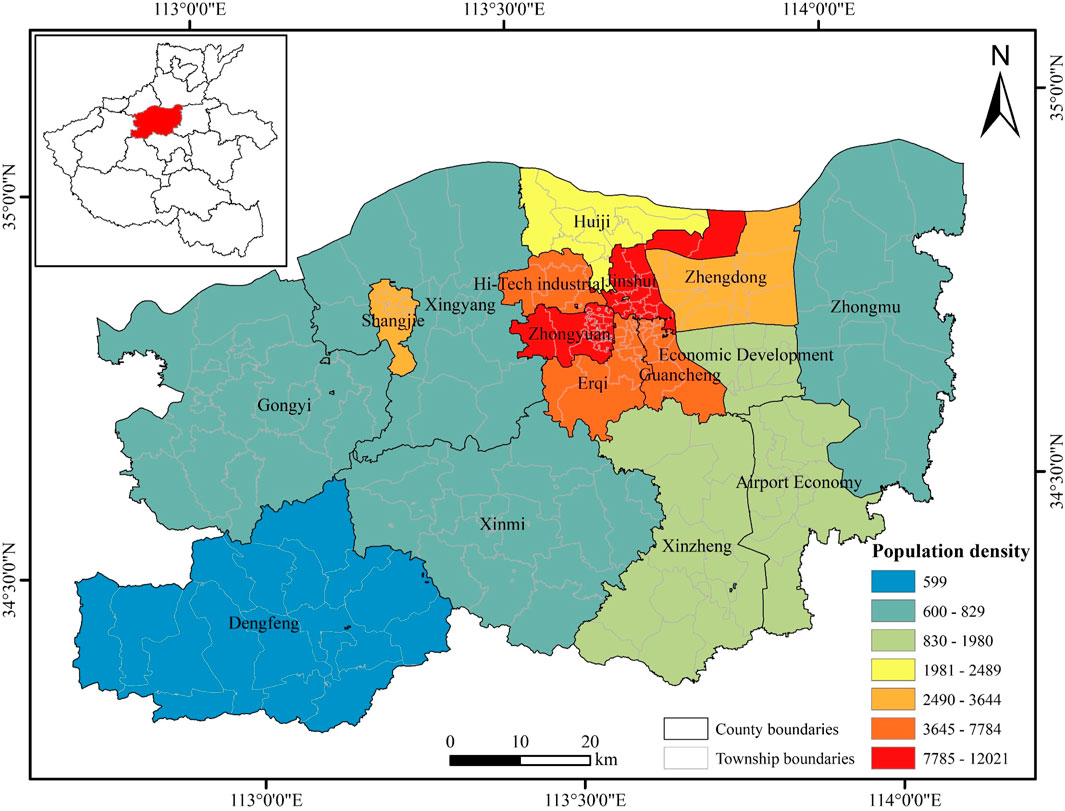
FIGURE 1. Study area in Henan, China, and county-level population density data.
2.2 Data sources
Choosing the appropriate model is the key to population spatialization, while the auxiliary data with good quality and high spatial-temporal consistency is an important factor to improve the accuracy of the population model. The spatial distribution of population is the result of the joint action of natural environmental factors and socio-economic factors in the region. Considering the above two factors, the details of the data sources used in this study are shown in Table 1.
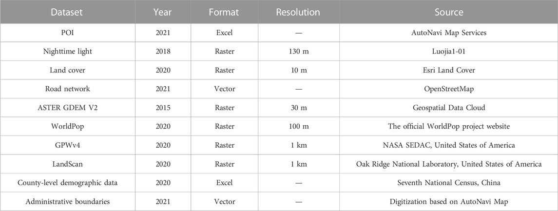
TABLE 1. List of data sources used in this study.
The distribution of the multi-source data in the study is illustrated in Figure 2. It can be seen that Luojia1-01 nighttime light data can clearly distinguish the structure and scope of the city, and the roads. The topography of Zhengzhou is high in the southwest and low in the northeast. Xingyang City, Shangdi District, Gongyi City, Dengfeng City, and Xinmi City are classified as the western region, while other districts and counties are classified as the eastern region. There are many high mountains and hills in the west, with the built area accounting for 32.93% of its total area, and the trees and scrubs/shrubs accounting for 23.16%. The eastern area is flat, with the built area accounting for 48.98% of its total area, and the trees and scrubs/shrubs accounting for 3.18%. Meanwhile, the road network density is high (4,520.95
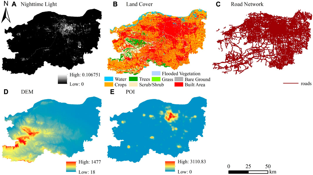
FIGURE 2. The distribution of the multi-source data in the study.
2.3 Data processing
(1) Population data. Gridded Population of the World (GPW) (https://sedac.ciesin.columbia.edu/) proportionally allocated total population to grid cells based on the assumption that population is distributed evenly over administrative units (Tian et al., 2005). LandScan (https://landscan.ornl.gov/) relied on ancillary data to spatially weighted population density within a given administrative unit (Stevens et al., 2015). These two datasets were chosen as validation data for accuracy assessment. WorldPop (https://www.worldpop.org/) used county-level census data for population redistribution and provided gridded population datasets with high accuracy at the finest spatial resolution (i.e., 100 m) in China (Stevens et al., 2015; Ye et al., 2019). Census work is conducted every 10 years in China. Township-level demographic data for the Seventh National Census data (China, 2020) in Zhengzhou are unavailable because they have not been released by government departments. Meanwhile, the data from the Sixth National Census (China, 2010) is too outdated, and after a decade of development, both the city’s administrative boundaries and population have changed considerably. The county-level population value was extracted from WorldPop data (mainland China dataset), and then the WorldPop data were linearly corrected based on the seventh county-level census data. Then, the township-level population was counted from the corrected WorldPop data by zoning statistics as township-level statistical population data, and then the population density of each township was calculated.
(2) Administrative boundary data. The 2020 district codes published by the China National Bureau of Statistics (http://www.stats.gov.cn/tjsj/tjbz/) and Baidu search were used to access information on the adjustment and renaming of townships (streets) and counties (districts) in Zhengzhou. Then, administrative boundary data were processed to match them with the seventh census data.
(3) POI data. Through API, POI data were obtained from the AutoNavi Map Services (https://lbs.amap.com/), one of the most commonly used navigation map services in China. Each POI contains information such as name, type, latitude and longitude, address, etc. There are 23 types of POI in total, which are consistent with the classification standards of the AutoNavi Map (https://lbs.amap.com/api/webservice/download). The POI data were filtered and checked, and 596,330 effective POI records were obtained. Kernel density estimation (KDE), with a bandwidth set as 2000 m, was adopted to convert each type of discrete POI point data to continued and smooth density surfaces in ArcGIS software. The density surfaces were presented as raster data at 150 m, 300 m, and 500 m resolutions for each type of POI, respectively.
(4) Nighttime light data. The data were downloaded free from the Luojia1-01 website (http://59.175.109.173:8888). The data were subjected to radiance calibration and were resampled to 150 m, 300 m, and 500 m by bilinear interpolation. The radiance calibration formula is as follows:
where L is the radiation correction value after absolute radiation calibration, the unit is
(5) Land cover data. Land cover data was download from Esri website (https://livingatlas.arcgis.com/landcover/), which was produced based on 10 m Sentinel-2 image and depth learning method. There are a total of eight categories of land cover in Zhengzhou: water, trees, grass, flooded vegetation, crops, scrub/shrub, built area, and bare ground. With the tabulate area tool of ArcGIS, the township-level values of various land cover areas were counted, and then the proportion of various land cover areas (the area index) was calculated. Similarly, the grid-level area indices were obtained.
(6) DEM data. The ASTER GDEM V2 data were downloaded from the Geospatial Data Cloud (http://www.gscloud.cn/search). The surface analysis tool was used to perform slope and aspect analysis to obtain the slope and aspect raster layers in ArcGIS. Then, the mean elevation, mean slope, and mean aspect of each township cell and grid cell were counted.
(7) Road network data. The roads were derived from the OpenStreetMap (https://www.openstreetmap.org/, last accessed: 23 July 2021), the biggest volunteer geographic information platform in the world. The length of the roads in each township cell and grid cell was counted, and then the road density (
The data processing in this paper was carried out in ArcGIS (ESRI, Inc., Redlands, CA, United States of America) software. The coordinates systems were unified to the Alberts Conical Equal Area Projection, and the boundary range of all data was matched with the administrative boundaries. The vector data of administrative boundaries and grids were overlaid with other multi-source data to obtain the township-level value and grid-level value of each feature by the zoning statistics method. Due to the differences in units and evaluation criteria, the township-level value and grid-level value of each feature were normalized. For convenience, the types of features and their codes are shown in Table 2.
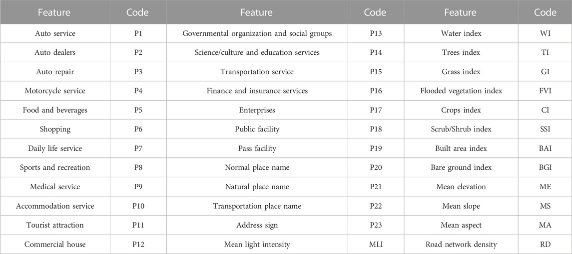
TABLE 2. Types of features and their codes in this study.
2.4 Methods
The flowchart of the population spatialization in the study is shown in Figure 3. It is divided into four parts.
(1) Data processing: Mosaicking, clipping, extraction by mask, reprojection, and resampling, etc. were performed on the acquired multi-source data.
(2) Feature extraction: The township-level value and grid-level value of each feature were obtained by methods such as zoning statistics method.
(3) Population mapping: Township-level feature values were used as independent variables and the township-level population density was used as the dependent variable, and both were input to the random forest model for training. Then, the grid-level feature values were input into the trained model to predict the population density of the grid cells. Then, the prediction layer of the grid was used as the weighting layer to disaggregate the census data into the grid to generate three-scale gridded population maps.
(4) Accuracy assessment: At the township level, the accuracy of three population maps was evaluated using statistical population data and validated against two publicly available population datasets, GPWv4 and LandScan.
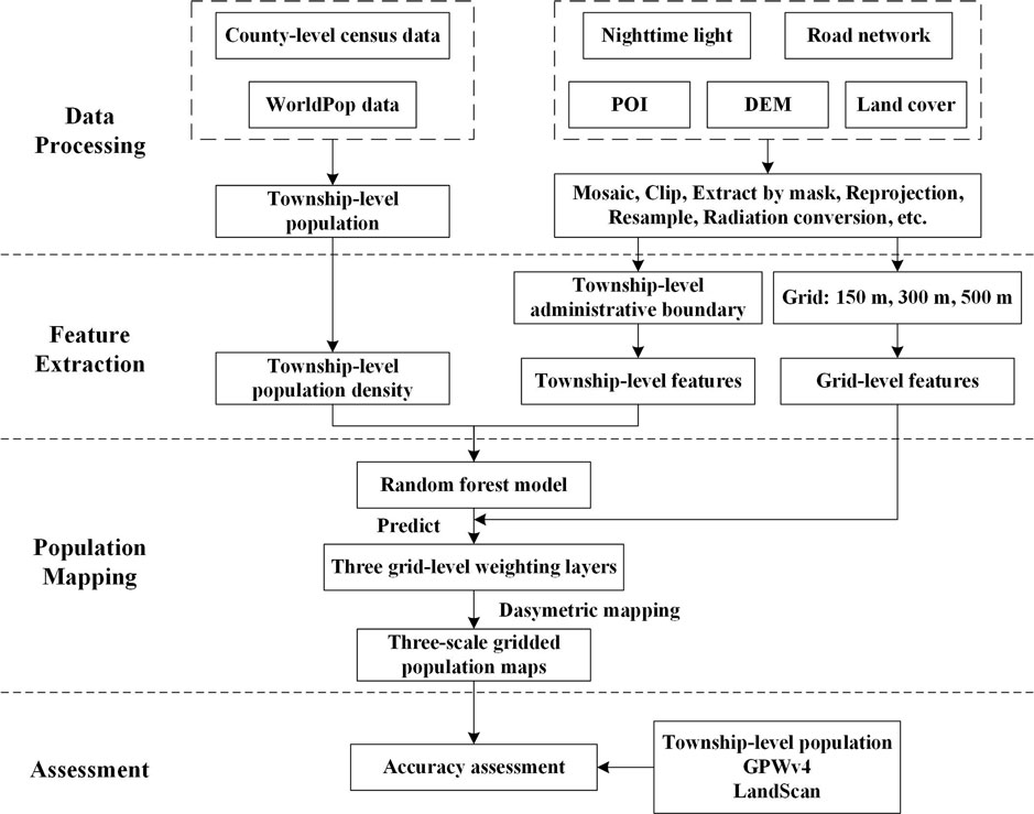
FIGURE 3. Flowchart of the population spatialization in the study.
2.4.1 Establishing random forest models
The random forest (RF) algorithm is an ensemble learning method composed of multiple independent decision trees. Taking advantage of the bootstrap resampling method, each tree in the random forest is trained by a random subset of training data, and the prediction results of all the trees are integrated as the output (Zhao et al., 2020). The random forest algorithm has the advantages of not needing to consider the multi-collinearity problem, avoiding the overfitting problem, having a high tolerance for outliers and noise, and being suitable for processing high-dimensional feature data (Chen and Zhao, 2020). The principle of random forest algorithm is as follows.
(1) There is a dataset
(2) Building a Classification and Regression Tree (CART). The features of the samples are used as nodes. When constructing the decision tree, how to select the segmentation variables (selected features) and segmentation points (segmentation that divides the feature space into two) is measured by the impurity of the nodes after segmentation. The mean square error (MSE) is used as a function to measure the impurity of nodes in the regression tree. The mean of the decreased impurity of each feature in all decision trees is used as a measure of the importance of the feature, which is called Mean Decrease Impurity. The impurity of this node is the weighted sum
where
The factors affecting population distribution can be divided into two categories: natural environmental factors and socio-economic factors. The natural environmental factors included mean elevation, mean slope, mean aspect, and 8 types of area indices; and the socio-economic factors included mean light intensity and road network density and 23 types of POI average kernel density, with a total of 36 features. The population density of 200 townships in Zhengzhou was used as the dependent variable, and the township-level normalized data for each feature were taken as the independent variables (feature matrix). The scikit-learn library was used in VSCode (Visual Studio Code) software based on Python to construct random forest models to fit the relationship between the population density and various types of features. Considering the problem that the raster resolution corresponds to the grid scale, three random forest models were constructed to realize the population map with three scales.
When training the random forest model, it is necessary to adjust the parameters of the model to make the model perform optimally on the given dataset. The performance of the model is evaluated by averaging the correct rate of ten-fold cross-validation method. The specific method is to divide the entire dataset into ten subsets and select one subset as the test set in turn and the remaining nine subsets as the training set. Then, this process is executed ten times until all subsets have been used once as the test sample. In this way, all samples are used as training set and test set, and each sample is verified once, which can well evaluate the generalization ability of the model. After adjusting the model parameters based on the above principles, the optimal parameters of the random forest models corresponding to the three grids are shown in Table 3 below. The random_state of all models was set to 10, and other parameters except the following three parameters remained a default. The term random_state controls both the randomness of the bootstrapping of the samples used when building trees. When random_state is fixed, the random forest generates a fixed set of trees, but each tree is still inconsistent. The term n_estimators represents the number of base estimators. Theoretically, the larger the n_estimators, the better the model effect and the longer the training time, but after it reaches a certain value, the accuracy of the model will reach a near steady state. The term max_depth represents the maximum depth of the tree, and branches that exceed the maximum depth will be pruned. The term max_features represents the number of features considered when limiting branching, and features that exceed the limit will be discarded. If the model is overfitting, the prediction results become poor. The depth of the tree is controlled by limiting the values of max_depth and max_features, which in turn prevents overfitting.
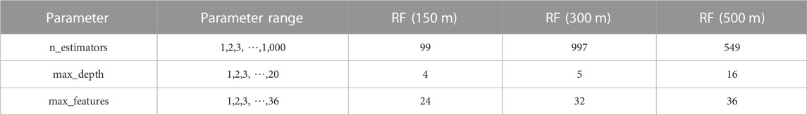
TABLE 3. Optimal values of parameters for three random forest models.
The dataset for constructing each decision tree is obtained by sampling with replacement. Some samples may appear multiple times in the same dataset, and some samples may not be sampled once. the samples that are not sampled are called out-of-bag data (OOB), accounting for about one-third of the training samples. A random forest model with optimal parameters was established by tuning the parameters. The complete data set was input into the model for training, and the out-of-bag data were used as the test set to test the accuracy of the model. The trained model was applied to the grids to predict the population density of each grid. Then the gridded population density layer was employed as a weighting layer for population redistribution.
2.4.2 Dasymetric mapping
Dasymetric mapping is a technique whereby ancillary data is employed to guide the redistribution of population data at a finer level of resolution (Chun et al., 2018; Bakillah et al., 2014; Briggs et al., 2007; Mennis, 2009). The idea is to use the auxiliary data to generate weight layers and use the weight layers to redistribute the census data (Sinha et al., 2019). In this study, the water body was regarded as unpopulated. At the same time, according to the characteristics of land cover in Zhengzhou City, there were large areas of trees and shrubs in the western alpine hills, so the grids containing only two types of land cover, trees and shrubs, were also regarded as unpopulated. The grid-level population density was used as the weighting layer to disaggregate the census data into the grid using Formula 3, as follows:
Where
In China, population and boundary data for villages and communities (a finer level than township) are unavailable due to the confidentiality of data, making it difficult to use more granular population data for accuracy assessment. Therefore, this paper selected county-level demographic data for population redistribution and conducted accuracy assessment at the township level.
2.4.3 Assessment method
The simulated population of all grids within each township cell was counted using the zoning statistics method, and the error between the township-level simulated population data and the township-level demographic data was calculated. The indicators of accuracy assessment are the mean absolute error (MAE), the root mean square error (RMSE), the relative error (RE), the mean relative error (MRE), and the coefficient of determination (
Where
3 Results
3.1 Population spatialization
After predicting the value of the grid cells by the trained random forest model, the value of the grid cells containing only three land cover types, water, trees, and shrubs, was assigned to 0, and then the population was corrected at the county level.
Figure 4 shows the three-scale gridded population distribution maps in Zhengzhou, which are recorded as 150PD, 300PD and 500PD respectively. The population distribution at three scales was well expressed, and the simulation of the 150PD dataset was more detailed. The three gridded population maps showed the same pattern of population distribution. The population distribution of Zhengzhou City showed the pattern of “one large core, multiple small core points”. Meanwhile, when compared with the nighttime light and POI maps (Figure 2), it showed that the high population area matches the locations of high brightness and high POI density. The population distribution in the central city was shown as “one large core.” There were 6,836,412 simulated population in the central city, with a population density of approximately 5,491 persons/
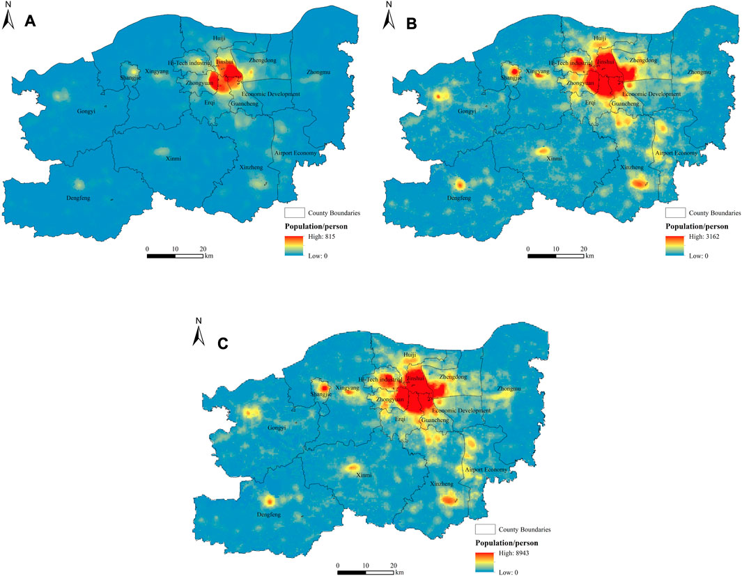
FIGURE 4. The three-scale gridded population distribution maps (datasets) in Zhengzhou: (A) population distribution map at the 150 m level (150PD); (B) population distribution map at the 300 m level (300PD); (C) population distribution map at the 500 m level (500PD).
Gongyi City, Dengfeng City, Shangjie District, Xingyang City, Xinmi City, and Zhongmu County all had a small core point of population distribution, with main population concentrated in their county seat. The population of Xinzheng was mainly distributed in the northern and southeastern parts of the city, the northern part of which was bordered by the central city and was densely populated by the radiation of the central city. The population of the Airport Economic Zone was distributed in a belt from north to south, with the construction of an urban integrated service area with a denser population in the north, Xinzheng International Airport as the core in the center, and a manufacturing cluster in the south. The land cover type of the core point area with concentrated population distribution is mainly built area with strong economic activities and sound infrastructure.
3.2 Accuracy assessment
Considering the availability and operability of the data, the GPWv4 and LandScan in 2020 were chosen for comparison at the township level. The errors were calculated according to the above Formulas 4, 5, 7. Table 4 shows the accuracy assessment indicators based on the MAE, RMSE, and MRE in five datasets at the township level. The MAE was 13,942.04 for 150PD, 14,185.81 for 300PD, 14,299.12 for 500PD, 29,290.96 for GPWv4, and 28,080.42 for LandScan, with RMSE values of 18,807.78, 18,954.64, 19,327.38, 41,927.81, and 40,498.94 attained, respectively. The MAE and RMSE of the three population datasets in this study were significantly lower than those of the GPWv4 and LandScan datasets. When compared with the MRE of LandScan (45.69%), there was a little greater error (53.19%) for the 500PD dataset and there were smaller ones for the 150PD and 300PD datasets (42.24% and 45.33%), and all four were smaller than the GPWv4 dataset (57.78%). The results show that the error of population simulation was smaller in this study, the degree of deviation was smaller between the simulated population and the statistical population, and the overall simulation error was slightly lower. And as the grid scale decreased, the error decreased, indicating that grid scales had different effects on the representation of the population.
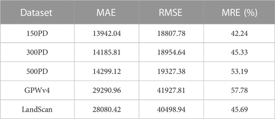
TABLE 4. Comparison of accuracy assessment in five population datasets.
The simulated population within each township was summed and linearly fitted with the statistical population at the township level. Figure 5 shows the correlations between the simulated population and the statistical population in 200 townships. Each point stands for the value of the simulated and corresponding statistical population at the township level. It can be seen that the data points of the 150PD, 300PD, and 500PD datasets were more concentrated near the regression line than GPWv4 and LandScan datasets. Moreover, when compared with the
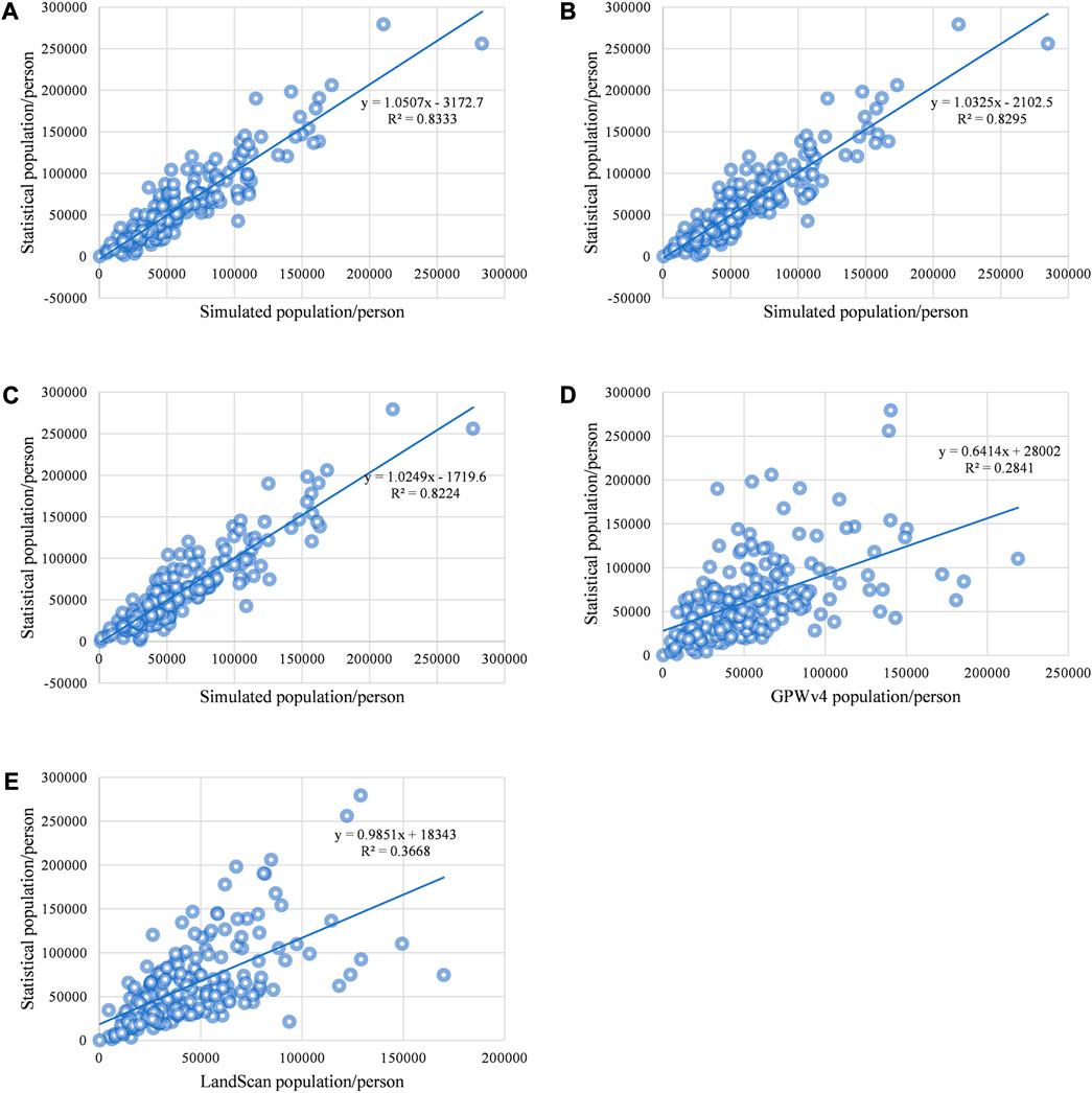
FIGURE 5. Comparison of the correlations between the simulated population and the statistical population in 200 townships: (A) 150PD dataset; (B) 300PD dataset; (C) 500PD dataset; (D) GPWv4; (E) LandScan.
The RE was calculated according to Formula 6 at the township level. The RE was divided into five ranges, and the number of townships with different error ranges was counted (Figure 6). The five ranges are severely underestimated (SUE;

FIGURE 6. The number of townships with different error ranges based on relative error.
To intuitively understand the distribution of relative errors geographically, the relative error distribution map at the township level derived from the 150PD dataset is shown (Figure 7). The underestimation error of population simulation reached a minimum of −0.56, but the overestimation error was larger in some townships, mainly in Jianshan Scenic Area Management Committee (Region a, RE was 12.43), Xinzhong Township (Region b, RE was 7.18), Liuhe Township (Region c, RE was 3.15), and Guzhishan National Forest Park Management Committee (Region d, RE was 2.89). These four townships are located in the western mountainous area of Zhengzhou City, and their land cover types are mainly trees and shrubs, accounting for 59.14% of the total area of the four townships; the built area only accounts for 26.90%. However, the built area of the central city accounts for 71.65% of its total area. The POI density is 278.14 points/
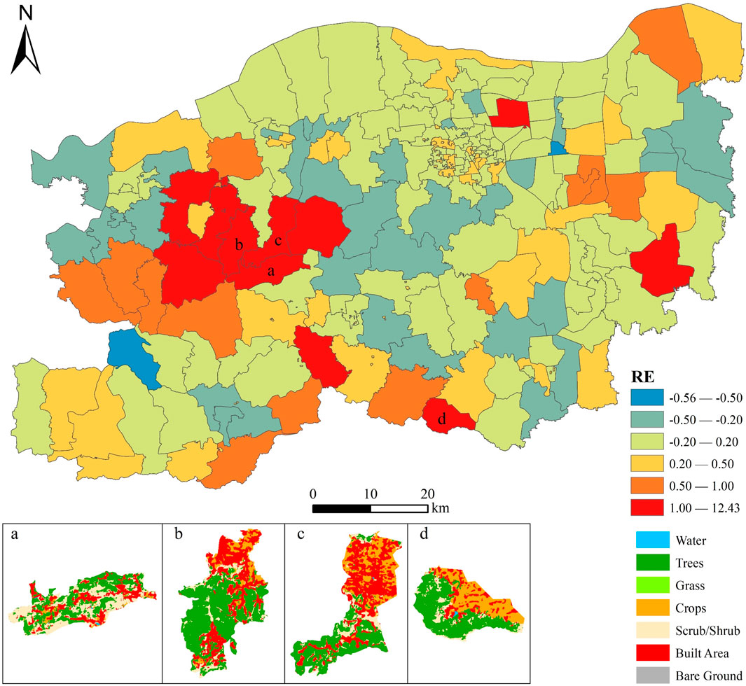
FIGURE 7. Relative error distribution at the township level (150PD dataset). (A-D) indicate regions, echoed in the figure.
3.3 Feature importance analysis
The Feature Importance Index (FII) output from the random forest model was used to evaluate the degree of influence of each feature on the population simulation. Figure 8 shows the ranking of FII from the output of the random forest model corresponding to the 150 m scale. The higher the value of the FII, the greater the influence of the feature. The total value of all the FII is 1. The top ten features were displayed in the red box. It can be seen that the top ten features were all derived from POI data. The spatial distribution of the top ten POI-related features is shown in Figure 9. These ten types of POI-related features had a similar spatial distribution pattern to the population, showing “high in the central city and multiple cores in the periphery.” There was high POI density and high population density in the central city.
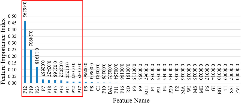
FIGURE 8. The ranking of feature importance index (FII).
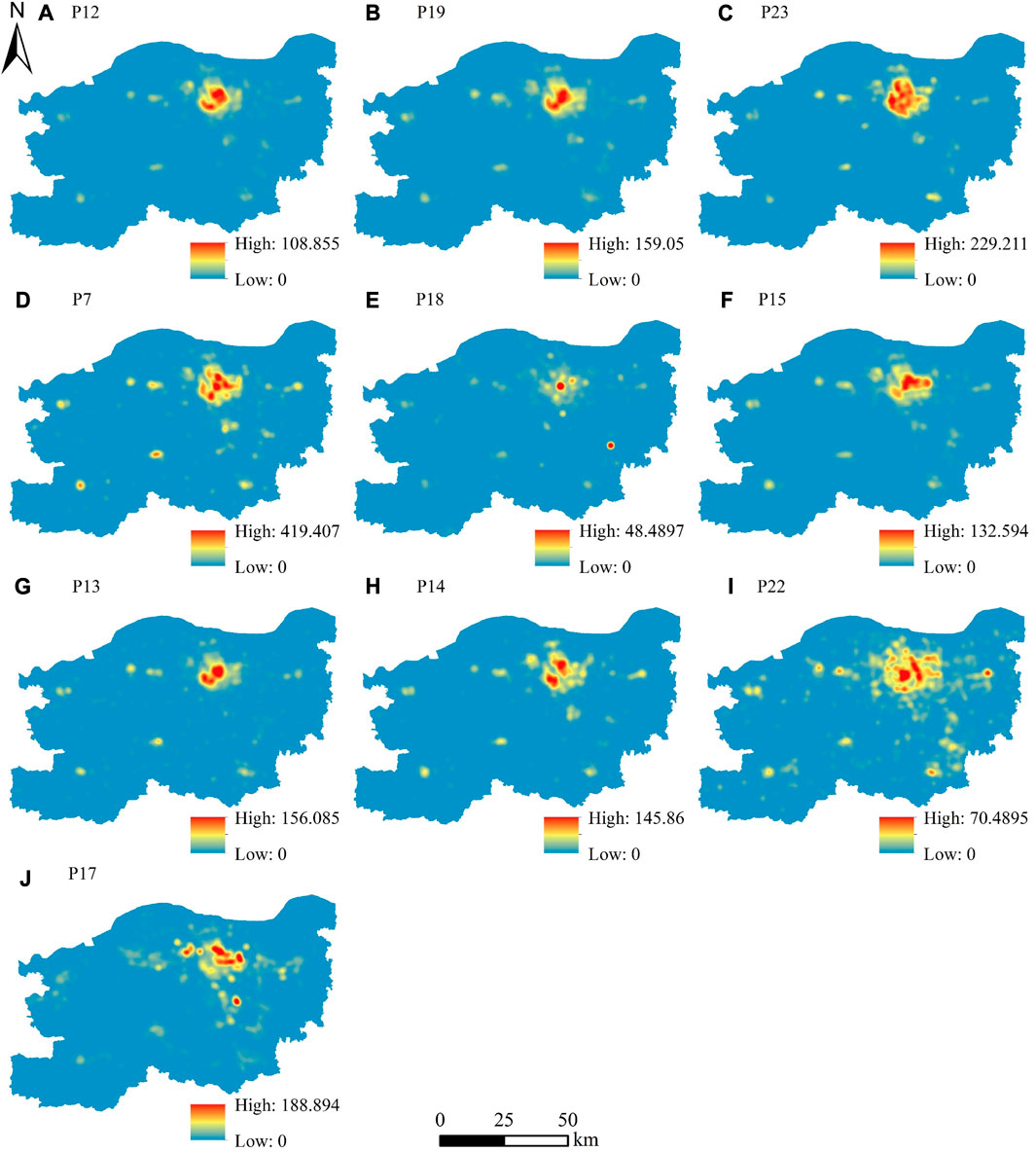
FIGURE 9. The spatial distribution of the top ten POI-related features.
The total FII of the top ten POI-related features was 0.96049, while the total FII of all POI-related features was 0.98907, indicating that POI-related features contributed significantly to the population simulation compared to other features. Commercial House (P12, 0.46592) had a much higher FII than other features. Commercial House (P12, 0.46592) contains the information of building and residential area; Pass Facility (P19, 0.24935) contains the information of the gates of buildings and street houses; Address Sign (P23, 0.11918) contains the information of building number. These three features reflected the building and residence information and ranked in the top three. Meanwhile, the sum of the FII of these three features was 0.83445, which indicates that the features related to residence information had greater contributions to the population simulation. Daily Life Service (P7, 0.02687), Public Facility (P18, 0.02427), Transportation Service (P15, 0.02168), Science/Culture and Education Services (P14, 0.01220), and Medical Service (P9, 0.00093) are part of infrastructure construction. The FIIs of these five infrastructure constructions ranked 4th, 5th, 6th, 8th, and 20th, respectively, which can be concluded that infrastructure construction was more correlated with population distribution. The density of POI for infrastructure construction was 73.58 points/
Topographic features include mean aspect (MA, 0.00036), mean slope (MS, 0.00035), and mean elevation (ME, 0.00030), which were ranked 27th, 29th, and 30th, respectively, in terms of FII. The topography of Zhengzhou is high in the southwest and low in the northeast, but the FIIs of topographic features are ranked low. The influence of topographic features is more pronounced at the provincial level and above, while less at the municipal level (Dong et al., 2016). Population distribution is closely related to land. While population distribution is affected by land cover types, human activities are also changing land cover types. In Zhengzhou, crops cover 42.02% of the total area, and built areas cover 39.94% of the total area. Among the features extracted from land cover data, the crops index (CI, 0.00383) and the built area index (BAI, 0.00275) had a greater impact on population simulation. The accuracy of population spatialization results based on nighttime lighting data is higher in densely populated urban areas, while the fit is poor for rural areas with low population density (Zeng et al., 2011; Wang and Zhang, 2021). The mean light intensity (MLI, 0.00067) could reflect the distribution characteristics of the population to some extent, but it was not expressive enough for the population distribution. The results indicate that the POI-related features contribute more to the population simulation compared to other features, which can cause the FIIs of other features to rank lower with smaller values.
4 Discussion
To understand the role of POI data on population spatialization, two groups of supplementary experiments (groups A and B) were done to generate two 150 m-level population maps for comparison with the 150PD dataset (group C) already generated in Figure 4A. In the case of retaining 13 features other than POI-related, group A is without POI-related features; group B is combining all POI data without considering the types of POI and calculating the average kernel density of POI as a feature; group C is considering 23 types of POI features. The experiment went well. Table 5 shows the comparison of the accuracy assessment indicators in the three groups of experiments. From A to C, the
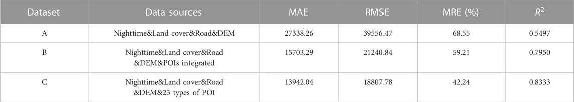
TABLE 5. Comparison of accuracy assessment indicators in the three groups of experiments.
Four regions in the three groups of gridded population maps were selected for comparative analysis (Figure 10): Region a with high population density and clustered distribution, region b with medium population density and small nucleation point distribution, region c with low population density and scattered population distribution, and region d with more concentrated population distribution along the valley. Meanwhile, the accuracy of the population spatialization results in this study was verified by combining Landsat-8 images. As can be seen from Figure 10, group A could simulate the geomorphic contours of population distribution, but could not reflect the density of population distribution in detail. After adding POI-related features (B and C), in regions a and b, the population distribution changed gradually from more to less from urban center to urban edge, and the simulated population in the grid increased, which reduced the underestimation of urban population; In region c, the population distribution did not change much because in rural areas with low population density and scattered distribution, the number of various types of POIs is small, while even the recorded POI data are incomplete; In region d, the population distribution expanded. The asymptotic distribution of the population in group C could be better represented compared to group B. From the above analysis, it can be concluded that adding POI-related features can not only simulate the geomorphic contour of population distribution but also can more reflect the spatial heterogeneity of population distribution, which can greatly enhance the change of population distribution and reduce the underestimation of the population in urban areas.

FIGURE 10. Regional comparison of three 150 m-level gridded population maps. (A-D) indicate the codes for each of the three groups of experiments.
Although the introduction of POI can greatly improve the accuracy of population spatialization, as a typical volunteer geographic information (VGI) data, more POI data are collected in urban areas than in rural areas, and many POI data in rural areas are unrecorded; this is beneficial for population simulation in urban areas and less useful for population simulation in rural areas (Neis and Zielstra, 2014; Ma et al., 2015; Zhao et al., 2020). The main factor describing the distribution of the population in rural areas is land cover data. In addition, there are some POIs for public facilities, accommodations, and restaurants in unpopulated landscapes, which bring errors to the population simulation. From the above analysis of FII, it was shown that POI features related to residence information play a larger role in population simulation. Humans inhabit the buildings. The building footprint data are used as a unit to simulate the population distribution, which will improve the accuracy of simulation and the level of detail of the simulated population distribution. The use of building footprint data for population spatialization will require more research in future studies, considering information on the location, profile, floor level, and usage of buildings, however detailed building footprint data are not readily available.
5 Conclusion
In this study, POI, LuoJia1-01 nighttime light, land cover, road network, and DEM data were selected as the factors that describe the population distribution. Random forest models were constructed to simulate the population distribution at three scales of 150 m, 300 m, and 500 m in Zhengzhou in 2020. The accuracy of the three population datasets of this study was assessed at the township level and compared and evaluated with the GPWv4 and LandScan datasets. The degree of contribution of each type of feature to the population simulation was analyzed based on the FII of the random forest model. Experimental analysis was then conducted around the POI data to explore the role of POI data and its types on the spatialization of the population. The main conclusions are as follows.
(1) The results of population spatialization in this study were in line with the actual situation of population distribution in Zhengzhou. The population distribution showed the pattern of “one large core, multiple small core points”, forming cores that break through the administrative boundaries and show a trend different from the distribution of administrative regions. The population density was high in the central city and low in the surrounding area.
(2) Compared with the GPWv4 and LandScan datasets, the simulation accuracy and performance of the three datasets in this study were better. And the smaller the scale of the grid, the higher the accuracy of population spatialization, with an accuracy ranking of 150PD > 300PD > 500PD > LandScan > GPWv4.
(3) POI data were proven to be important factors indicating population distribution, and those related to residence information had greater contributions to population spatialization. Meanwhile, the introduction of POI can greatly improve the accuracy of population spatialization and reduce the underestimation of the urban population, and typed POI data were more favorable for population spatialization.
Although the effect of population spatialization in this study is good, there are still some limitations. 1) The same random forest model was used for the entire study area in each experiment, which resulted in large overestimation errors for some townships in the mountainous areas of western Zhengzhou. In future studies, zonal modeling will be carried out to reduce the errors caused by large differences in regional conditions. To further improve the simulation accuracy of population distribution, the integration of other factors with finer scales, such as building footprint data, could also be considered. 2) The Sixth Census data is too outdated, and township-level population data from the Seventh Census has not been published. Therefore, township-level population data were obtained by correcting WorldPop dataset and then counting it. This data has a certain deviation from the actual township-level census data, which has a certain impact on the accuracy of the simulation results. After the release of the township-level population data of the Seventh National Census, this data can be used for the research of population spatialization to make the accuracy assessment more reliable.
Data availability statement
The original contributions presented in the study are included in the article/supplementary material, further inquiries can be directed to the corresponding author.
Author contributions
GC and LL contributed to the conception and design of the study. LL, JY, and YC completed the data collection and processing as well as the experimental content. GC, LL, JY, and YC contributed to original draft preparation. GC and LL contributed to review and editing of the manuscript. All authors contributed to the article and approved the submitted version.
Funding
This research was funded by the Fundamental Research Funds for the Universities of Henan Province (NSFRF180329); the MOE (Ministry of Education in China) Project of Humanities and Social Sciences (15YJCZH018); Science and Technology Project of Henan Province (162102210063).
Acknowledgments
We would like to thank the reviewers for contributing to improve this manuscript, as well as the editors for their kind suggestions and professional support.
Conflict of interest
The authors declare that the research was conducted in the absence of any commercial or financial relationships that could be construed as a potential conflict of interest.
Publisher’s note
All claims expressed in this article are solely those of the authors and do not necessarily represent those of their affiliated organizations, or those of the publisher, the editors and the reviewers. Any product that may be evaluated in this article, or claim that may be made by its manufacturer, is not guaranteed or endorsed by the publisher.
References
Bai, Z. Q., Wang, J. L., and Yang, F. (2013). Research progress in spatialization of population data. Prog. Geogr. 32 (11), 1692–1702. doi:10.11820/dlkxjz.2013.11.012
Bakillah, M., Liang, S., Mobasheri, A., Arsanjani, J. J., and Zipf, A. (2014). Fine-resolution population mapping using openstreetmap points-of-interest. Int. J. Geogr. Inf. Sci. 28 (9), 1940–1963. doi:10.1080/13658816.2014.909045
Briggs, D. J., Gulliver, J., Fecht, D., and Vienneau, D. M. (2007). Dasymetric modelling of small-area population distribution using land cover and light emissions data. Remote Sens. Environ. 108 (4), 451–466. doi:10.1016/j.rse.2006.11.020
Chen, F. L., and Zhao, G. W. (2020). Fine-scale simulation of population distribution based on zoning strategy and machine learning. Sci. Surv. Mapp. 45 (9), 165–173. doi:10.16251/j.cnki.1009-2307.2020.09.025
Cheng, L. X., Wang, L. Z., Feng, R. Y., and Yan, J. N. (2021). Remote sensing and social sensing data fusion for fine-resolution population mapping with a multimodel neural network. IEEE J. Sel. Top. Appl. Earth Observations Remote Sens. 14, 5973–5987. doi:10.1109/JSTARS.2021.3086139
Chun, J., Zhang, X. C., Huang, J. F., and Zhang, P. C. (2018). A gridding method of redistributing population based on POIs. Geogr. Geo-Information Sci. 34 (04), 83–89+124+2. doi:10.3969/j.issn.1672-0504.2018.04.013
Clark, C. (1951). Urban population densities. J. R. Stat. Soc. Ser. A(General) 114 (4), 490–496. doi:10.2307/2981088
Dong, N., Yang, X. H., and Cai, H. Y. (2016). Research progress and perspective on the spatialization of population data. J. Geo-information Sci. 18 (10), 1295–1304. doi:10.3724/SP.J.1047.2016.01295
Fu, J. Y., Jiang, D., and Huang, Y. H. (2014). A dataset of population distribution on a kilometer grid in China. Acta Geogr. Sin. 69 (S1), 41–44. doi:10.3974/geodb.2014.01.06.v1
Guo, B., Bian, Y., Zhang, D. M., Su, Y., Wang, X. X., Zhang, B., et al. (2021). Estimating socio-economic parameters via machine learning methods using luojia1-01 nighttime light remotely sensed images at multiple scales of China in 2018. IEEE Access 9, 34352–34365. doi:10.1109/ACCESS.2021.3059865
He, M., Xu, Y. M., and Li, N. (2020). Population spatialization in Beijing city based on machine learning and multisource remote sensing data. Remote Sens. 12 (12), 1910. doi:10.3390/rs12121910
Hu, Y. F., Zhao, G. H., and Zhang, Q. L. (2018). Spatial distribution of population data based on nighttime light and LUC data in the Sichuan-Chongqing Region. J. Geo-information Sci. 20 (1), 68–78. doi:10.12082/dqxxkx.2018.170224
Jiang, D., Yang, X. H., Wang, N. B., and Liu, H. H. (2002). Study on spatial distribution of population based on remote sensing and GIS. Prog. Geogr. 17 (5), 734–738.
Li, K. N., Chen, Y. H., and Li, Y. (2018). The random forest-based method of fine-resolution population spatialization by using the international space station nighttime photography and social sensing data. Remote Sens. 10 (10), 1650. doi:10.3390/rs10101650
Li, Y. X., and Liu, M. H. (2021). Spatialization of population based on Xgboost with multi-source data. IOP Conf. Ser. Earth Environ. 783, 012083–12125. doi:10.1088/1755-1315/783/1/012083
Lo, C. P. (2008). Population estimation using geographically weighted regression. GIScience Remote Sens. 45 (2), 131–148. doi:10.2747/1548-1603.45.2.131
Ma, D., Sandberg, M., and Jiang, B. (2015). Characterizing the heterogeneity of the OpenStreetMap data and community. ISPRS Int. J. Geo-Information 4 (2), 535–550. doi:10.3390/ijgi4020535
Martin, D. (1996). An assessment of surface and zonal models of population. Int. J. Geogr. Inf. Syst. 10 (8), 973–989. doi:10.1080/02693799608902120
Mennis, J. (2009). Dasymetric mapping for estimating population in small areas. Geogr. Compass 3 (2), 727–745. doi:10.1111/j.1749-8198.2009.00220.x
Mennis, J. (2003). Generating surface models of population using dasymetric mapping. Prof. Geogr. 55 (1), 31–42. doi:10.1111/0033-0124.10042
Neis, P., and Zielstra, D. (2014). Recent developments and future trends in volunteered geographic information research: The case of OpenStreetMap. Future Internet 6 (1), 76–106. doi:10.3390/fi6010076
Ou, J. P., Liu, X. P., Liu, P. H., and Liu, X. J. (2019). Evaluation of luojia1-01 nighttime light imagery for impervious surface detection: A comparison with NPP-VIIRS nighttime light data. Int. J. Appl. Earth Observation Geoinformation 81, 1–12. doi:10.1016/j.jag.2019.04.017
Sinha, P., Gaughan, A. E., Stevens, F. R., Nieves, J. J., Sorichetta, A., and Tatem, A. J. (2019). Assessing the spatial sensitivity of a random forest model: Application in gridded population modeling. Comput. Environ. Urban Syst. 75, 132–145. doi:10.1016/j.compenvurbsys.2019.01.006
Stevens, F. R., Gaughan, A. E., Linard, C., and Tatem, A. J. (2015). Disaggregating census data for population mapping using random forests with remotely-sensed and ancillary data. PLoS ONE 10 (2), e0107042. doi:10.1371/journal.pone.0107042
Sun, L., Wang, J., and Chang, S. P. (2021). Population spatial distribution based on luojia 1-01 nighttime light image: A case study of beijing. Chin. Geogr. Sci. 31 (6), 966–978. doi:10.1007/s11769-021-1240-6
Tian, Y. Z., Yue, T. X., Zhu, L. F., and Clinton, N. (2005). Modeling population density using land cover data. Ecol. Model. 189 (1-2), 72–88. doi:10.1016/j.ecolmodel.2005.03.012
Wang, L. T., Wang, S. X., Zhou, Y., Liu, W. L., Hou, Y. F., Zhu, J. F., et al. (2018). Mapping population density in China between 1990 and 2010 using remote sensing. Remote Sens. Environ. 210, 269–281. doi:10.1016/j.rse.2018.03.007
Wang, L. Y., Fan, H., and Wang, Y. K. (2020). Improving population mapping using Luojia 1-01 nighttime light image and location-based social media data. Sci. Total Environ. 730, 139148. doi:10.1016/j.scitotenv.2020.139148
Wang, M. L., and Zhang, H. S. (2021). Research on population spatialization based on luojia-1 nighttime light data. Geospatial Inf. 19 (09), 53–56+7. doi:10.3969/j.issn.1672-4623.2021.09.013
Xiao, D. S., and Yang, S. (2019). A review of population spatial distribution based on nighttime light data. Remote Sens. Land Resour. 31 (03), 10–19. doi:10.6046/gtzyyg.2019.03.02
Xiong, J. N., Li, K., Cheng, W. M., Ye, C. C., and Zhang, H. (2019). A method of population spatialization considering parametric spatial stationarity: Case study of the southwestern area of China. ISPRS Int. J. Geo-Information 8 (11), 495. doi:10.3390/ijgi8110495
Yang, X. R., and Chen, N. (2019). Spatialization of population data for fujian Province based on multi-source data. J. Guizhou Univ. Nat. Sci. 36 (02), 79–84+95. doi:10.15958/j.cnki.gdxbzrb.2019.02.16
Yao, Y., Liu, X. P., Li, X., Zhang, J. B., Liang, Z. T., Mai, K., et al. (2017). Mapping fine-scale population distributions at the building level by integrating multisource geospatial big data. Int. J. Geogr. Inf. Syst. 31 (6), 1–25. doi:10.1080/13658816.2017.1290252
Ye, T. T., Zhao, N. Z., Yang, X. C., Quyang, Z. T., Liu, X. P., Chen, Q., et al. (2019). Improved population mapping for China using remotely sensed and points-of-interest data within a random forests model. Sci. total Environ. 658, 936–946. doi:10.1016/j.scitotenv.2018.12.276
Zeng, C. H., Zhou, Y., Wang, S. X., Yan, F. L., and Zhao, Q. (2011). Population spatialization in China based on night-time imagery and land use data. Int. J. Remote Sens. 32 (24), 9599–9620. doi:10.1080/01431161.2011.569581
Zeng, W. J., Zhong, Y. D., Li, D. L., and Deng, J. Y. (2021). Classification of recreation opportunity spectrum using night lights for evidence of humans and POI data for social setting. Sustainability 13 (14), 7782. doi:10.3390/su13147782
Zhang, J. Q., Shi, W. B., and Xiu, C. L. (2021). Urban research using points of interest data in China. Sci. Geogr. Sin. 41 (1), 140–148. doi:10.13249/j.cnki.sgs.2021.01.015
Zhao, S., Liu, Y. X., Zhang, R., and Fu, B. J. (2020). China’s population spatialization based on three machine learning models. J. Clean. Prod. 256, 120644. doi:10.1016/j.jclepro.2020.120644
Keywords: population spatialization, random forest model, typed poi data, luojia1-01 nighttime light, multi-source
Citation: Liu L, Cheng G, Yang J and Cheng Y (2023) Population spatialization in Zhengzhou city based on multi-source data and random forest model. Front. Earth Sci. 11:1092664. doi: 10.3389/feart.2023.1092664
Received: 08 November 2022; Accepted: 25 July 2023;
Published: 03 August 2023.
Edited by:
Juergen Pilz, University of Klagenfurt, AustriaReviewed by:
Vikas Kamal, EHS Guru Sustainable Solutions Private Limited, IndiaChigozie Edson Utazi, University of Southampton, United Kingdom
Copyright © 2023 Liu, Cheng, Yang and Cheng. This is an open-access article distributed under the terms of the Creative Commons Attribution License (CC BY). The use, distribution or reproduction in other forums is permitted, provided the original author(s) and the copyright owner(s) are credited and that the original publication in this journal is cited, in accordance with accepted academic practice. No use, distribution or reproduction is permitted which does not comply with these terms.
*Correspondence: Gang Cheng, Y2hlbmdnYW5nMTIxOEAxNjMuY29t