An algorithm for correction of atmospheric scattering dilution effects in volcanic gas emission measurements using skylight differential optical absorption spectroscopy

Differential Optical Absorption Spectroscopy (DOAS) is commonly used to measure gas emissions from volcanoes. DOAS instruments measure the absorption of solar ultraviolet (UV) radiation scattered in the atmosphere by sulfur dioxide (SO₂) and other trace gases contained in volcanic plumes. The standard spectral retrieval methods assume that all measured light comes from behind the plume and has passed through the plume along a straight line. However, a fraction of the light that reaches the instrument may have been scattered beneath the plume and thus has passed around it. Since this component does not contain the absorption signatures of gases in the plume, it effectively “dilutes” the measurements and causes underestimation of the gas abundance in the plume. This dilution effect is small for clean-air conditions and short distances between instrument and plume. However, plume measurements made at long distance and/or in conditions with significant atmospheric aerosol, haze, or clouds may be severely affected. Thus, light dilution is regarded as a major error source in DOAS measurements of volcanic degassing. Several attempts have been made to model the phenomena and the physical mechanisms are today relatively well understood. However, these models require knowledge of the local atmospheric aerosol composition and distribution, parameters that are almost always unknown. Thus, a practical algorithm to quantitatively correct for the dilution effect is still lacking. Here, we propose such an algorithm focused specifically on SO₂ measurements. The method relies on the fact that light absorption becomes non-linear for high SO₂ loads, and that strong and weak SO₂ absorption bands are unequally affected by the diluting signal. These differences can be used to identify when dilution is occurring. Moreover, if we assume that the spectral radiance of the diluting light is identical to the spectrum of light measured away from the plume, a measured clean air spectrum can be used to represent the dilution component. A correction can then be implemented by iteratively subtracting fractions of this clean air spectrum from the measured spectrum until the respective absorption signals on strong and weak SO₂ absorption bands are consistent with a single overhead SO₂ abundance. In this manner, we can quantify the magnitude of light dilution in each individual measurement spectrum as well as obtaining a dilution-corrected value for the SO₂ column density along the line of sight of the instrument. This paper first presents the theory behind the method, then discusses validation experiments using a radiative transfer model, as well as applications to field data obtained under different measurement conditions at three different locations; Fagradalsfjall located on the Reykjanaes peninsula in south Island, Manam located off the northeast coast of mainland Papua New Guinea and Holuhraun located in the inland of north east Island.

1 Introduction

Volcanic plumes are common occurrences at active volcanoes around the world. These plumes contain volatile species exsolved from magma rising from depth. The chemical signature of volcanic plumes depends on magma chemistry, the interaction of rising volatiles with rocks and water, and potentially condensation and re-evaporation from hydrothermal systems. Plumes may contain gases and aerosols, with the latter consisting of cloud droplets, ash, and secondary aerosols from the oxidation of volcanogenic gas species. The gas phase of high-temperature volcanic plumes predominantly consists of water vapor (H₂O), carbon dioxide (CO₂), and sulfur dioxide (SO₂), with lesser amounts of hydrogen sulfide (H₂S), hydrogen halides (HCl, HF, HBr), and a variety of minor trace components including hydrogen, helium, reduced carbon species, and metals/metalloids (Giggenbach 1996; Gerlach 2004; Oppenheimer et al., 2014). Tracking changes in the emission rate and composition of gas emissions can provide crucial information on volcanic processes occurring at depth and provide input into eruption forecasts (e.g., Aiuppa et al., 2007, 2021; Burton et al., 2007; de Moor et al., 2016a, 2016b; Kunrat et al., 2022). Furthermore, volcanic plumes can be transported long distances from their sources, causing impact on air quality, air traffic, fumigation of soils and water bodies, health, and infrastructure. Therefore, routine monitoring of volcanic plumes has become one of the key components of modern volcanic and atmospheric surveillance (Sparks et al., 2012; Kern et al., 2022).

The most commonly measured gas species in volcanic plumes is SO₂. This is because this species is a marker of magmatic activity, the background concentration in air is usually of a few parts per billion (ppb), and measurement is facilitated by passive remote sensing techniques sensitive to the strong light absorption of SO₂ in the near ultraviolet wavelengths. Since the 1970s, correlation spectroscopy (COSPEC) has been used to measure SO₂ remotely from ground by analysis of the absorption of diffused solar light at discrete narrow wavelength bands in the 305–330 nm spectral range (Moffat and Millán, 1971). This technique has been gradually replaced by differential optical absorption spectroscopy (DOAS), which instead analyses the absorption features of a continuous spectrum in the same range (Galle et al., 2003). The technique is now used at dozens of volcanoes for routine monitoring with stationary scanning DOAS systems, or by traversing under the plume with zenith-looking DOAS instruments (Edmonds et al., 2003; Johansson et al., 2008; Galle et al., 2010; Platt et al., 2015; Arellano et al., 2021).

The DOAS method is based on absorption spectroscopy and uses the UV-light from the Sun, scattered within the atmosphere as it travels to the instrument. The conventional application of the method assumes that all the measured light comes from above the plume and has passed through the plume in route to the instrument. The last scattering event of the measured light occurs above the plume and, from there, crosses the plume along the instrument’s line of sight. However, a fraction of the light that reaches the instrument may come from atmospheric scattering without first passing through the plume. This light causes a “dilution” of the amount of gas measured. In clean-air conditions and with short distance between the instrument and the plume, this dilution effect is small, but if conditions get hazier, and/or the distance to the plume increases, this effect may become severe. Thus, as elevated plumes or opaque atmospheres are common on many volcanoes, this effect is regarded as a major error source in volcanic SO₂ emission monitoring using UV spectroscopy (Millán, 1980; Mori et al., 2006; Kern et al., 2010).

Already in the COSPEC era it was recognized that this atmospheric scattering could severely affect the measurements of gas emissions from volcanoes and industrial sources (Millán, 1980). Now that the mini-DOAS systems are commonly applied to quantify volcanic gas emissions, this problem has received increased attention (Mori et al., 2006; Kern et al., 2010), and the error in typical emission rate measurements due to atmospheric scattering is today estimated to be 10%–100% depending on geometric and meteorological conditions. Several attempts have been made to model the phenomena (Kern et al., 2012), and the physical mechanisms are now relatively well understood. However, applying such models to retrieve volcanic emission rates requires knowledge of the local aerosol composition and distribution, both inside the plume and in the background atmosphere, parameters that are rarely known with the required accuracy. Thus, practical algorithms to quantitatively correct for the effect are needed. We here propose one such algorithm.

Mori and collaborators recognized that when DOAS measurements of SO₂ in volcanic plumes were made over longer distances, atmospheric scattering between the instrument and the plume caused underestimation in the derived SO₂ columns and that this dilution was stronger at shorter wavelengths and at higher SO₂ columns (Mori et al., 2006). They suggested that evaluating SO₂ columns in different wavelength bands in the region 303–320 nm could be used to qualitatively detect if there is significant underestimation in the DOAS measurements due to atmospheric scattering. Fickel and Delgado Granados also conclude that different wavelength bands yield different column densities, and suggested using evaluation in longer wavelength bands, when possible, to minimize but not eliminate the dilution effect (Fickel and Delgado Granados, 2017). Varnam et al. (2020) suggested a method for quantitative correction of the atmospheric scattering dilution based on evaluation in two different wavelength bands in the range 306–322 nm. They use synthetically modelled spectra (Esse et al., 2020), with varying SO₂ column and atmospheric scattering dilution. These spectra were then evaluated in the two wavelength bands and the results were used to build a look-up table. The results from evaluating measured plume spectra in the same two wavelength bands were then compared with the corresponding data in the look-up table, providing a dilution factor that facilitates a quantitative correction of the measured plume spectra.

The approach to quantify the scattering effect described here is based on taking advantage of the non-linearity of the Beer-Lambert law for absorption, as well as the difference in light intensity in the plume spectrum caused by SO₂ broadband absorption, combined with the assumption that the spectral distribution of the light scattered below the plume is similar to the spectral distribution of the light scattered without the plume. The method is applicable when multiple scattering inside the plume can be neglected (low amounts of ash and other aerosols). The method is more robust when the measured gas columns are high enough to cause significant non-linearity and broadband intensity reduction in the absorption spectra studied.

2 Experimental details

The basic mini-DOAS system consists of a pointing telescope fiber-coupled to a spectrograph. The narrow field of view telescope gathers ultraviolet light from the Sun, scattered from aerosols and molecules in the atmosphere. Light is transferred from the telescope to the spectrometer by an optical fiber. The spectra are digitalized and logged on a computer for analysis using DOAS (Platt and Stutz, 2008). In this way, the slant column density of various gases in the viewing direction of the telescope is derived (Galle et al., 2003). Two different setups are commonly used, the MobileDOAS and the ScanningDOAS.

In the MobileDOAS setup measurements are made from a mobile platform. The telescope is pointing towards zenith while traversing under the plume at the same time as the position of the platform is logged by a GPS. In this way the total number of SO₂ molecules in a cross-section of the plume may be derived, and after multiplication with the wind speed at plume height the emission in kg s^-1 is obtained.

In the ScanningDOAS setup the telescope is motorized to automatically scan the field of view of the instrument over 180°. In a typical measurement the instrument is located under the plume, and scans are made, from horizon to horizon, in a plane perpendicular to the wind-direction. Thus, automatic unattended measurements of the SO₂ emission with 5–10 min time resolution can be made. This is the concept used in the NOVAC network (Galle et al., 2010).

In this paper we focus on the MobileDOAS application. In the MobileDOAS application measurements of sky and plume are made in the same zenith direction, while in the ScanDOAS application the plume spectra are taken in varying directions different from the clean air sky spectrum which may complicate the use of the here suggested algorithm.

A correct unit to use for column measurement of a gas is molec/cm². In our case, volcanic gas emissions, this means numbers of the order 10¹⁶–10¹⁹. In connection with COSPEC measurements a more practical unit, ppm m, was introduced and has become widely used in the volcano gas community, yielding results in the order 10–10,000 ppm m. It should be noted, however, that the instruments measure mass units not mixing ratio. Nevertheless, we define 1 ppm m as 2.5∙10¹⁵ molec/cm² (its true value for STP) and for clarity use this unit throughout this paper. Thus, to convert any data in this paper expressed in ppm m to mass units one should simply multiply with 2.5∙10¹⁵, without any correction for pressure or temperature.

3 Methods

3.1 Qualitative description

The conventional DOAS method applied in routine remote sensing of volcanic SO₂ assumes that all the measured light has been last scattered into the field of view above the plume and has passed in a straight line through the plume. In practice, however, a fraction of the light that reaches the instrument originates from atmospheric scattering on molecules and aerosols below the plume and thus has not passed through the plume. This causes a “dilution” of the slant column retrieved by the DOAS method.

We define the following:

• Sky spectrum: a spectrum of the skylight that has not passed through the plume. This can be measured in a location with plume free zenith view.

• Plume spectrum: a spectrum of the skylight that has passed through the volcanic plume but not undergone dilution afterwards. Not directly measurable.

• Dilution spectrum: a spectrum of skylight that is scattered into the field-of-view of the measurement device from the atmosphere below the plume and has thus never passed through the plume. Not directly measurable.

• Measured spectrum: the spectrum as observed by the instrument while aimed at the volcanic plume, hence the combined plume and dilution spectrum.

• Dilution factor k: the fraction of the sky spectrum, that is obtained after iterative subtraction of fractions of the sky spectrum (normalized as described in Section 3.2) from the measured spectrum.

Figure 1 shows a theoretical SO₂ transmittance spectrum covering the region commonly used in DOAS evaluations, with the three narrow evaluation intervals used in this paper highlighted (305–310, 310–315, and 315–320 nm). When a certain fraction of the measured light has not passed through the plume, it will dilute the measured spectrum and act to reduce the measured absorption. If we assume that the spectral shape of this diluting light is identical to that of the sky spectrum, then the different absorption bands will be diluted with the same fraction. However, if the absorption is strong enough that the absorption features in the shorter wavelength bands, which have the strongest absorption, do not respond linearly to the dilution, then this dilution of the measured spectrum will change the differential absorptions more in the shorter wavelength bands compared to the longer wavelength bands where the absorption is weaker. Hence, performing a DOAS evaluation of the different bands highlighted above will give different SO₂ column in each band (Fickel and Delgado Granados, 2017).

FIGURE 1

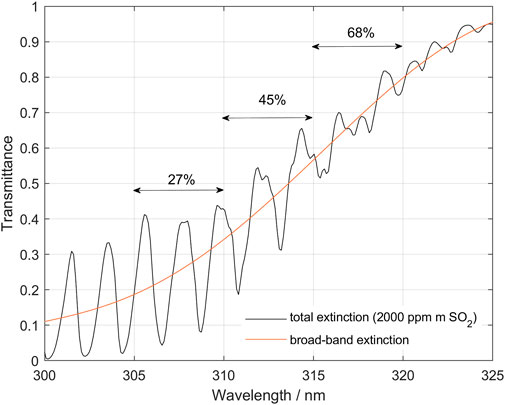
FIGURE 1. Theoretical transmittance spectrum for light passing through 2,000 ppm m SO₂. Notice that SO₂ broadband absorption is unequal for the three wavelength bands: 305–310, 310–315 and 315–320, which causes different dilution effects. Here it can be seen that due to the broad-band absorption in SO₂ the actual average intensity in the plume at the three wavelength bands used is only 27%, 45% and 68% respectively of the plume intensity without SO₂.

Also, the SO₂ broadband absorption contributes to this imbalance because although the different bands have equal absolute dilution, expressed as the ratio of the dilution to the sky spectrum, the effective intensity of light coming from the plume is different in the different bands and thus the relative dilution, with respect to the measured spectrum, will differ. Figure 1 shows the absorbance spectrum of 2,000 ppm m SO₂. Here it can be seen that due to the broadband absorption in SO₂ the actual intensity in the plume at the three wavelength bands used is only 27, 45, and 68%, respectively, of the plume intensity without SO₂. Thus, a dilution factor of 0.1 (10% of the normalized sky spectrum contribution to the measured spectrum), will effectively result in a dilution of the differential SO₂ absorption corresponding to about 37, 22, and 15% in the respective wavelength bands. Note that if there is no dilution then this difference in intensity between the evaluation bands caused by the broadband SO₂ absorption is not a problem as it is taken care of by the DOAS evaluation procedure. However, when dilution is present, this difference in intensity contribution from the plume results in a different effective dilution between the bands. In the following we refer to this effect as an “imbalance” in the absorption and make use of this effect to indicate presence of “below-the-plume” scattering and quantitatively correct for its diluting effect. As will be discussed further later in this paper, some other wavelength dependent processes, like plume aerosol extinction and atmospheric ozone concentration, may also contribute to the “imbalance” when dilution is present.

The method presented here relies on the assumption that the fraction of diluting light, i.e., the ratio of the light scattered below the plume, the dilution spectrum, to the spectrum of light scattered above the plume, the sky spectrum, is constant within a narrow spectral interval. By narrow we mean a band not wider than 10 nm.

The method is applied as follows: first, we perform conventional DOAS evaluations on two adjacent or slightly overlapping bands encompassing an interval at least 5 nm and not larger than 10 nm wide (e.g., 305–310 and 310–315 nm) to derive the apparent columns of SO₂ in the two bands, using a measured spectrum outside of the plume as the background. If there is dilution below the plume and the actual SO₂ column is sufficiently high, then the two retrieved columns will differ with the column retrieved at the stronger absorption band being lower than that from the weaker absorption band and both being lower than the true column. Notice that the spectral fit obtained at both bands may still look good (no significant systematics in the fit residual) because the effect of dilution on the spectral shape in such narrow spectral intervals is often not evident. If a difference in columns is found between the two bands, we proceed to iteratively subtract a constant fraction of the sky spectrum from the measured spectrum until a fraction is found where the evaluated columns in the two bands coincide. To obtain a quantifiable parameter for the dilution, the sky spectrum used in the iterative subtraction is normalized to become of equal intensity to the measured spectrum at 350 nm, which is chosen to be close to the SO₂ absorption region but not significantly affected even by strong absorptions of SO₂. Hereby we quantitatively obtain the amount of spectral dilution (the dilution factor k, see above) as well as a corrected value for the column. The process is described in more detail and with illustrations in Figures 2, 3.

FIGURE 2

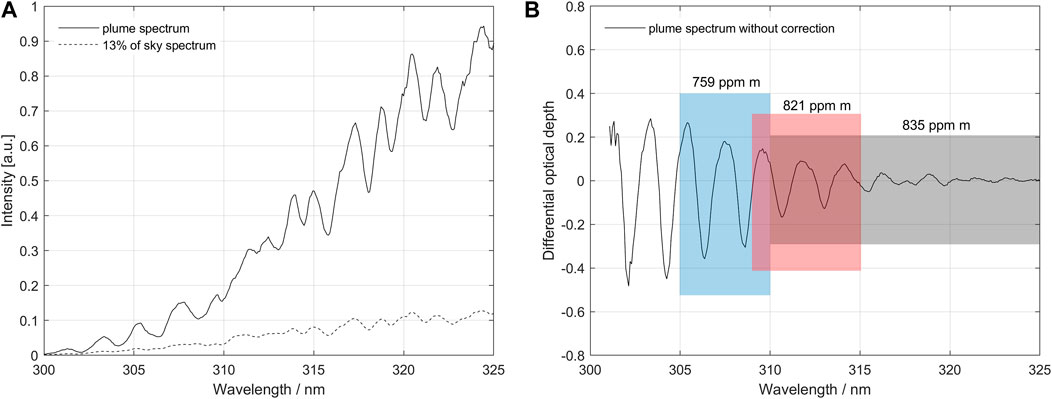
FIGURE 2. (A) Example of a measurement affected by dilution taken on a traverse on 18 March 2013 at Turrialba volcano, Costa Rica. The measured plume spectrum contains an unknown fraction of scattered sunlight from below the plume, the dilution spectrum. The picture also shows a dilution spectrum scaled in intensity to be 13% of the sky spectrum at 350 nm. (B) Differential absorption optical depth spectrum derived from the original spectra. The standard evaluation using DOAS in the fit-region of 310–325 nm gives a slant column density (SCD) of 835 ppm m. Evaluations in fit-regions 1 (305–310 nm) and 2 (309–315 nm) give 759 and 821 ppm m, respectively. This imbalance is caused by below-the-plume-scattering, in combination with the logarithmic dependence of the Beer-Lambert law, and intensity variation in the plume spectrum caused by SO₂ broadband absorption.

FIGURE 3

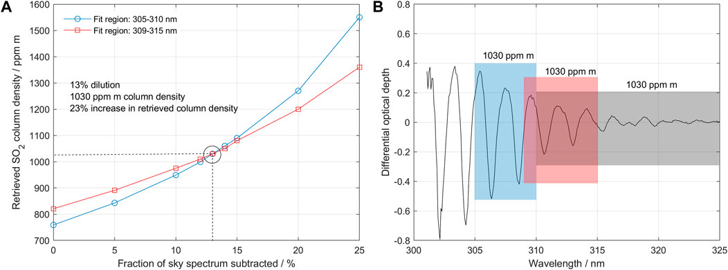
FIGURE 3. (A) Retrieved SCDs using fit regions 1 and 2 as a function of the amount of scattered light that has been subtracted from the original measured spectrum. A subtraction of 13% scattered light yields equal values in both fit regions of 1,030 ppm m. This is defined as a dilution factor of 0.13. (B) Differential absorption optical depth spectrum after subtraction of 13% scattered light. Now all fit regions yield the same SCD value of 1,030 ppm m. After applying the scattering correction algorithm, the slant column is increased by 23% from 835 (standard evaluation) to 1,030 ppm m.

3.2 Formalization

In the following we formalize the method. For the sake of clarity, we assume that any instrumental effect that may be present in the plume and sky spectra, such as dark current, offset spectra, or possible changes in the instrumental line function or wavelength calibration, have been corrected.

We can represent the algorithm mathematically in the following way: the measured spectrum, ${\mathrm{I}}_{\mathrm{m}}\left(\lambda \right)$ is expressed as the sum of the plume spectrum, ${\mathrm{I}}_{\mathrm{p}}\left(\lambda \right)$, and the dilution spectrum, ${\mathrm{I}}_{\mathrm{d}}\left(\lambda \right)$:

${\mathrm{I}}_{\mathrm{m}}\left(\lambda \right)={\mathrm{I}}_{\mathrm{p}}\left(\lambda \right)+{\mathrm{I}}_{\mathrm{d}}\left(\lambda \right)(1)$

It is convenient to relate the measured spectrum to the sky spectrum. Both may be measured under different conditions, for instance at different elevation angles or under unequal background scattering conditions. This results in intensities that may vary even in spectral intervals where absorption by the plume is expected to be negligible. We can start by defining a ‘scaled sky spectrum’ as the product of the sky spectrum by a factor equal to the ratio of the intensities of the measured and sky spectrum at a wavelength with negligible SO₂ absorption. We choose the intensities averaged over 5 nm at 350 nm for this scaling:

${\mathrm{I}}_{\mathrm{S}}^{\prime }\left(\lambda \right)={\mathrm{I}}_{\mathrm{s}}\left(\lambda \right)\left[\frac{{\mathrm{I}}_{\mathrm{m}}\left(350nm\right)}{{\mathrm{I}}_{\mathrm{s}}\left(350nm\right)}\right](2)$

The scaling is not problematic because it is equivalent to allowing a free scaling between the measured spectrum and the sky spectrum in the standard DOAS formalism.

The dilution spectrum is assumed to be proportional to the scaled sky spectrum ${\mathrm{I}}_{\mathrm{s}}\left(\lambda \right)$ within a narrow wavelength interval:

${\mathrm{I}}_{\mathrm{d}}\left(\lambda \right)=\mathrm{k}{\mathrm{I}}_{\mathrm{S}}^{\prime }\left(\lambda \right)(3)$

With the constant $\mathrm{k}$ > 0 defined as the dilution factor.

The plume spectrum must then correspond to the complementary fraction $\left(1-k\right)$ of the scaled sky spectrum multiplied by a Beer-Lambert law term with a relative optical depth $\mathrm{\tau }\left(\lambda \right)$ between the plume and scaled sky spectra. This relative optical depth not only contains the effect of absorption by SO₂ in the plume but also the effect of all other processes that make both spectra different, namely: difference in O₃ absorption, difference in elastic and inelastic (Ring effect) molecular scattering, or difference in extinction due to aerosols.

${\mathrm{I}}_{\mathrm{p}}\left(\lambda \right)=\left(1-k\right){\mathrm{I}}_{\mathrm{S}}^{\prime }{\left(\lambda \right)\mathrm{e}}^{-\mathrm{\tau }\left(\lambda \right)}(4)$

The meaning of the complementary factor $\left(1-k\right)$ is to normalize the transmittance of the measured spectrum with respect to the scaled sky spectrum. We do this by noting that in the limit of zero relative optical depth the measured and scaled sky spectrum must be equal.

Then follows that the measured spectrum is equal to:

${\mathrm{I}}_{\mathrm{m}}\left(\lambda \right)={\mathrm{I}}_{\mathrm{S}}^{\prime }\left(\lambda \right)\left[\left(1-k\right){\mathrm{e}}^{-\mathrm{\tau }\left(\lambda \right)}+\mathrm{k}\right](5)$

The method we propose iteratively subtracts a fraction of the normalized sky spectrum ${\mathrm{I}}_{\mathrm{s}}^{\prime }\left(\lambda \right)$ from the measured spectrum ${\mathrm{I}}_{\mathrm{m}}\left(\lambda \right)$, normalizes the new transmittance spectrum to compensate for the subtracted term, and applies the DOAS retrieval on two adjacent wavelength intervals. In each iteration, we find a set of fit parameters that minimize the difference between the logarithms of the modelled and measured spectra. These parameters are the coefficients of a polynomial that represents broadband structures of the relative optical depth (between scaled sky and measured spectra), and the relative column densities of atmospheric gases or pseudo-absorbers (O₃, Ring-effect) with absorption features in the interval of evaluation, as well as an apparent column density of SO₂, ${\mathrm{S}}_{\mathrm{i}}$.

Let us use the notation ${\mathrm{R}}_{\mathrm{i},\Delta \mathrm{\lambda }}\left({\mathrm{I}}_{\mathrm{m}}\left(\lambda \right)\right)\to {\mathrm{S}}_{\mathrm{i},\Delta \mathrm{\lambda }}$ to represent the retrieval of an apparent column density ${\mathrm{S}}_{\mathrm{i}}$ at a spectral interval $\Delta \mathrm{\lambda }$ applied to the spectrum ${\mathrm{I}}_{\mathrm{m}}\left(\lambda \right)$. We apply the retrieval in two adjacent narrow spectral intervals on modified spectra formed by subtracting a fraction of the scaled sky spectrum from the measured spectrum, followed by re-normalization:

${\mathrm{R}}_{\mathrm{i},\Delta \mathrm{\lambda }}\left(\frac{{\mathrm{I}}_{\mathrm{m}}\left(\lambda \right)-{\mathrm{x}}_{\mathrm{i}}{\mathrm{I}}_{\mathrm{s}}^{\prime }\left(\lambda \right)}{1-{\mathrm{x}}_{\mathrm{i}}}\right)\to {\mathrm{S}}_{\mathrm{i},\Delta \mathrm{\lambda }}(6)$

This iteration is applied until we find the constant fraction ${\mathrm{x}}_{\mathrm{i}}$ that would make the retrieved columns ${\mathrm{S}}_{\mathrm{i}}$ at the two adjacent spectral intervals equal. In other words, we vary x_i until ${\mathrm{S}}_{\mathrm{i},\Delta \mathrm{\lambda }1}={\mathrm{S}}_{\mathrm{i},\Delta \mathrm{\lambda }2}$. We can see from equations [1–5] that this occurs when ${\mathrm{x}}_{\mathrm{i}}=\mathrm{k}$, i.e., when we subtract from the measured radiance the component that was added by scattering of radiation not passing through the plume. In this way, we find not only the true column $\mathrm{S}$, but also the dilution factor $\mathrm{k}$, assumed to be constant along the two wavelength intervals used in the analysis.

3.3 Further considerations

Depending on the available amount of UV-light and actual SO₂ column strength, different wavelength intervals can be chosen for the evaluation. The idea is to select two wavelength intervals $\Delta \mathrm{\lambda }1$ and $\Delta \mathrm{\lambda }2$, wide enough to facilitate a good DOAS evaluation (∼5 nm), located close enough to encounter a similar dilution effect from atmospheric scattering, while still having a distinct difference in absorption cross-section. In addition, the absorption cross-section should be large enough so that at least one of the included absorption bands encounters non-linearity due to the Beer-Lambert law, given the actual SO₂ columns. Ideally, the intervals would also be differently affected by broadband SO₂ absorption. These conditions imply that different pairs may be optimal under different conditions; optically weak plumes need to be measured at short wavelengths to obtain enough non-linearity effects in the absorption, while optically thicker plumes, may need to be measured at longer wavelengths and thus weaker absorption as the stronger absorption bands may be saturated.

For the method to be able to determine a corrected column and dilution factor it is necessary that the difference between the columns derived using the two different bands can be clearly distinguished so that a well-defined cross-over point can be established. Thus, the true column and dilution must be high enough that the Beer-Lambert law non-linearity or SO₂ broad-band absorption cause a difference between the columns in the bands used that overcomes the noise level. This is illustrated in Figure 4, which shows how the columns derived in the three evaluation bands: 305–310, 310–315, and 315–320 nm are affected by dilution, for SO₂ columns of 500, 1,000 and 2000 ppm m, respectively. These plots are based on theoretical data. In a real case a difference between the columns of 5–10 ppm m is needed to overcome the noise level.

FIGURE 4

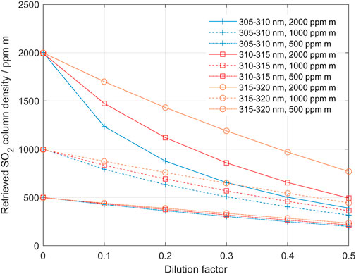
FIGURE 4. The underestimation of derived SO₂ column as a function of dilution, when using the different evaluation bands; 305–310 nm (blue), 310–315 nm (red) and 315–320 (orange) for SO₂ columns of 500, 1,000 and 2,000 ppm m, respectively. By following a pair of evaluated columns from high to low dilution the behavior of the iterative process in the dilution correction algorithm can be studied (see, for example Figure 3 above and Figure 11 below).

For SO₂ columns below 500 ppm m, the columns derived from the two lower bands, 305–310/310–315, respond almost linearly to increased dilution and the method will not converge and thus will fail to quantify the dilution. However, the dilution is still there and affects the column data linearly (15% dilution gives approximately 15% lower SO₂ column). For SO₂ columns higher than about 600 ppm m the difference between the two lower bands, at 10% dilution, is more than 10 ppm m and thus this pair can be used for evaluation of the dilution. In the same way, for SO₂ columns higher than about 800 ppm m also the higher pair 310–315/315–320 gives an imbalance response enough for evaluation at 10% dilution. At the other end, for SO₂ columns higher than 5,000 ppm m, saturation effects due to the limited spectral resolution start to cause problems for the lower pair. The longer-wavelengths pair is for the same reason limited to about 8,000 ppm m. Thus, for low to moderate SO₂ columns (600–2,000 ppm m) the lower pair is preferred due to its higher sensitivity, provided that the UV light level is high enough at 305 nm to overcome the noise level. For medium to high SO₂ columns (1,000–5,000 ppm m) the higher pair may instead be used, especially when the UV level at 305–310 nm is too low for accurate measurements. Of course, it is not possible to know the actual column before the correction, therefore evaluation at three bands may be necessary to explore the range of variation before choosing the pair of wavelength intervals that would maximize the quality of the retrieval based on the considerations given above.

In the examples and discussion above we assumed a dilution of 10%. With less dilution even higher true SO₂ columns are needed to give a reliable detection. This is also illustrated in Figure 4. The band with weakest absorption (315–320 nm) drops almost linearly with increasing dilution, while the band with the strongest absorption drops off faster than linearly initially and then drops more linearly, almost in parallel to the weak band. This is because with increasing dilution, the apparent column gets smaller and smaller and eventually the stronger absorption bands also become linear. By following the two curves belonging to a specific true SO₂ column from high to low dilution, one can simulate how the dilution correction method works. Notably, in the case of strong dilution (for example 50%) and strong true SO₂ column (for example, 2,000 ppm m), the apparent columns in the two stronger absorption bands initially diverge when dilution is decreased and then, as dilution continues to decrease, the lines of retrieved columns at the two bands start to converge. Thus, the iterative correction algorithm must allow for both convergence and divergence until the retrieved values are close enough and the column obtained at the weaker band is not lower than that obtained at the stronger band.

It is also interesting to note that, although the two processes of non-linearity and broad-band absorption both act to enhance the imbalance described above, the two processes in a way counterbalance each other. Figure 5 shows how the apparent SO₂ column, evaluated in the evaluation window 309–314 nm, varies with true SO₂ column for different dilution factors.

FIGURE 5

FIGURE 5. The apparent SO₂ column, evaluated in the evaluation band 309–314 nm, as a function of true SO₂ column, for different dilution factors.

For a given dilution constant, the effect of dilution due to broad-band SO₂ absorption becomes stronger and stronger with increasing SO₂ column density at the same time as the monotonous increase in apparent column due to non-linearity gets smaller and smaller. This results in a turnover making the apparent column decrease with increasing true SO₂ column. As a consequence, for a given evaluation band and dilution factor there is a maximum column that can be obtained in a DOAS evaluation. This effect has been pointed out by others (Mori et al., 2006; Varnam et al., 2020) and constitutes a limitation in standard DOAS evaluations as well as in some existing schemes for dilution correction. However, this is not a limitation for our method, as we just keep iterating until we reach the convergence point.

Besides the effect of dilution, conditions where light with dramatically different SO₂ column are superimposed in a single spectrum may also cause such an imbalance. This can occur when spectra containing different columns are co-added into a single spectrum, or if the field-of-view of the receiving optics cover a wider angle than represented by typical variations in total column in the plume, e.g., when a single spectrum contains light from both strong and weak columns. A typical example of this situation is when measurements are made at the beginning and end of a traverse where dramatic changes in column occur over short traverse distances. These effects can, to some extent, be avoided by using a narrow field-of-view and high sampling rate, and by excluding data from the traverse edges in the scattering correction dilution estimate.

Other processes resulting in similar effects are straylight in the spectrometer and scattering within the plume itself. The amount of straylight in the spectrometer depends on type of spectrometer as well as its condition and can to some extent be reduced by filtering out light with wavelengths outside the studied wavelength region. Moreover, the impact that straylight has on the imbalance can be checked by performing a measurement with a gas cell using a clean air background, with high enough gas column in the cell to reveal imbalance in the extinction law, with a nominal column value of 1,000 ppm m or more. If an imbalance in the absorption is detected in this cell measurement, straylight is likely to be present.

Eliminating effects of scattering within the plume is more difficult. One approach to study the impact of scattering within the plume on the spectral imbalance used in our method is modelling. The results from a study using the radiative transfer model McArtim (Deutschmann et al., 2011) is shown in the chapter 5.1 below. This modelling study indicates that the method presented here may give somewhat reduced column densities, especially for the case of a non-condensing plume above an opaque atmosphere. Plumes with high aerosol optical depths tend to offset this effect producing higher columns, probably due to multiple scattering.

A crucial condition in the method is that the clean air spectrum used in the iterative subtraction, and the true dilution spectrum caused by scattering below the plume, have similar shape over the two wavelength intervals used in the analysis. If this condition is not fulfilled, then the “crossover point” between the bands in the iterative process will be wrong. This problem is minimized by using two narrow wavelength bands located close to each other and to perform the sky and plume measurements close in time. Special care should be taken when cloud conditions differ significantly between sky and plume measurements. One way to check this is to compare the slope of the spectra in the actual wavelength interval, after dividing sky spectra taken before and after the plume traverse. Ozone has strong broadband absorption in the spectral regions suggested here and a difference in ozone between the sky spectrum and the plume spectrum may have an impact on the imbalance between the two evaluation bands. However, the impact of ozone is dominated by its stratospheric slant column density (O₃SCD), which is determined by the solar zenith angle (SZA, Eq. 6). Thus, if the sky spectrum is taken close in time to the plume spectrum, or if measurements are made close to noon, then the impact of ozone is negligible. If these conditions are not fulfilled, then the effect of ozone may still be eliminated by evaluating the relative ozone slant column density before and after passing the plume in the traverse. Using GPS data, time, and location, one can then derive the SZA related to each of these measurements and calculate the ozone vertical column density (O₃VCD) for the time of the traverse. Knowing the O₃VCD one can then use the GPS data of each spectrum to derive the O₃SCD of each spectrum and use the known absolute ozone absorption cross-sections to eliminate the effect of the difference in O₃SCD between the sky spectrum and the plume spectrum (including the dilution spectrum).

If we denote:

${{\mathrm{O}}_3\mathrm{S}\mathrm{C}\mathrm{D}}_{\mathrm{s}\mathrm{k}\mathrm{y}}$ ozone slant column density in sky spectrum

${{\mathrm{O}}_3\mathrm{S}\mathrm{C}\mathrm{D}}_{\mathrm{p}\mathrm{l}\mathrm{u}\mathrm{m}\mathrm{e}}$ ozone slant column density in plume spectrum

${\mathrm{O}}_3\mathrm{V}\mathrm{C}\mathrm{D}$ ozone vertical column density (common to sky and plume)

$\mathrm{S}\mathrm{Z}\mathrm{A}$ solar zenith angle (different for sky and plume)

${\mathrm{O}}_3\mathrm{V}\mathrm{C}\mathrm{D}=\frac{{{\mathrm{O}}_3\mathrm{S}\mathrm{C}\mathrm{D}}_{\mathrm{p}\mathrm{l}\mathrm{u}\mathrm{m}\mathrm{e}}-{{\mathrm{O}}_3\mathrm{S}\mathrm{C}\mathrm{D}}_{\mathrm{s}\mathrm{k}\mathrm{y}}}{\frac{1}{\cos {\mathrm{S}\mathrm{Z}\mathrm{A}}_{\mathrm{p}\mathrm{l}\mathrm{u}\mathrm{m}\mathrm{e}}}-\frac{1}{\cos {\mathrm{S}\mathrm{Z}\mathrm{A}}_{\mathrm{s}\mathrm{k}\mathrm{y}}}}(\mathrm{6a})$

3.4 Software

The method described above has been implemented in software, ScatteringCorrection, written in C++ and the initialization parameters are further described in the Supplementary Annex to this article. The software reads measured spectra saved in the extended standard (*.std) format, e.g., used by the MobileDOAS software (Johansson, 2009) and, for each measured spectrum, performs DOAS evaluations in two aforementioned narrow wavelength intervals and in one wider wavelength interval. If the SO₂ column in the wide wavelength interval exceeds a user-defined limit (approx. 500 ppm m), determined from when the non-linearity of the Beer-Lambert law begins, and there is a difference in SO₂ column between the two short wavelength intervals, then the software will attempt to perform a dilution correction of the measurement as described above.

The software performs a search for the optimal dilution factor k by attempting to minimize the difference between the evaluated SO₂ columns in the bands of longer and shorter wavelengths λ₁ and λ₂. ${\mathrm{S}}_{\mathrm{i},\Delta \mathrm{\lambda }1}$ < ${\mathrm{S}}_{\mathrm{i},\Delta \mathrm{\lambda }2}$ implies the applied dilution factor k is too small, while ${\mathrm{S}}_{\mathrm{i},\Delta \mathrm{\lambda }1}$ > ${\mathrm{S}}_{\mathrm{i},\Delta \mathrm{\lambda }2}$ implies k is too large. This fact is used to determine the direction of the search in each step of the iteration in which k is varied. Notice, however, that if the search has stepped too far beyond the optimum dilution factor k, the above relationship may fail. This fact must be accounted for in the search, most easily by also verifying that the DOAS fit is valid, e.g., by requiring a maximum permissible standard deviation in the fit residual. In our implementation, the search begins by attempting to determine the upper bound for k by stepping up k in relatively large steps until ${\mathrm{S}}_{\mathrm{I},\Delta \mathrm{\lambda }1}$ > ${\mathrm{S}}_{\mathrm{i},\Delta \mathrm{\lambda }2}$. During this stepping up of k, the software also determines the largest lower bound on the dilution factor, as the largest k_i, which yielded ${\mathrm{S}}_{\mathrm{i},\Delta \mathrm{\lambda }1}$ < ${\mathrm{S}}_{\mathrm{i},\Delta \mathrm{\lambda }2}$. The second phase of the search is to determine the optimum dilution factor k between the upper and lower bounds. In the case of valid DOAS fits for both the lower and upper bounds, this is done using a linear interpolation between the two as this method has been found to be the fastest. In the case of an invalid fit on either bound, which typically occurs when the upper bound has stepped too far, a binary search is applied instead.

4 Results

4.1 Modelling

To improve our understanding on how different parameters like plume height, SO₂ concentration, and aerosol burden in and below volcanic plumes influence our light dilution correction, we applied the method to spectra simulated with the radiative transfer model McArtim (Deutschmann et al., 2011). The model can be used to simulate UV/vis spectra expected in a wide range of user-defined atmospheric and plume conditions, and thus allows us to test the ability to derive accurate SO₂ SCDs using our scattering correction technique. For the purposes of this study, the spectra produced by the model were adapted to standard DOAS std format and then analyzed using the developed ScatteringCorrection program (see details in Supplementary Annex).

We study three scenarios: 1) a clean Rayleigh atmosphere and a plume with zero aerosol optical depth (clean atmosphere/clean plume); 2) the same plume but in an opaque atmosphere where a 1 km thick layer with aerosol optical depth of 0.2 is placed at ground level (opaque atmosphere/clean plume); and 3) an opaque plume with aerosol optical depth of 1, immersed in a clean atmosphere (clean atmosphere/opaque plume). For the three scenarios the plume has a vertical column density of 2,000 ppm m and has a cylindrical shape with 500 m diameter and horizontal orientation. The plume altitude is varied between 0 and 3,000 m above ground level (plume-bottom), which is assumed to be at 50 m above sea level. The Sun shines with a relative azimuth of 90° with respect to the plume axis and a solar zenith angle of 30°. The field of view of the instrument is set to 8 mrad. The instrument is located below the plume axis at 50 m altitude and pointed to the zenith. Other parameters of the simulation are given in the Supplementary Appendix.

Dividing each spectrum of the three scenarios by the respective clean air “sky” spectrum produces transmittance spectra, as shown in Figure 6.

FIGURE 6

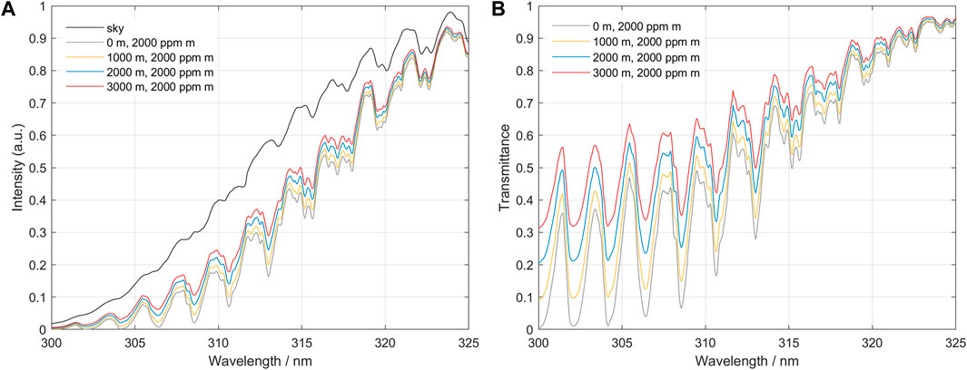
FIGURE 6. (A) Simulated spectra: a clean air “sky” spectrum and simulated measurement spectra of an SO₂ plume located at 0, 1,000, 2,000 and 3,000 m above ground level. We can see clearly that spectra from higher plumes have higher intensity due to added light from dilution. (B) The spectra from various plume heights, divided by the clean air “sky” reference. Note the spectral distortion for the spectra from elevated plumes, as well as the SO₂ broadband absorption.

Some correction algorithms have been proposed on the assumption that the diluting light follows the Koschmieder formula using either a Rayleigh scattering coefficient, or another coefficient suggested by the measurement conditions (Koschmieder, 1938; Mori et al., 2006; Vogel et al., 2011; Campion et al., 2015; Varnam et al., 2020). One way to test the assumptions of our model, that assumes a wavelength-independent dilution term, and the predictions of a wavelength-dependent term, is to test predictions of both on synthetic spectra. Our proposed model assumes that the dilution spectrum is a constant fraction of the sky spectrum, whereas in other methods the dilution spectrum is equal to the sky spectrum scaled by a wavelength dependent scattering efficiency. Using the spectra simulated with McArtim in which the true SO₂ column density is known we derived the wavelength-dependency of the dilution factor k (Figure 7).

FIGURE 7

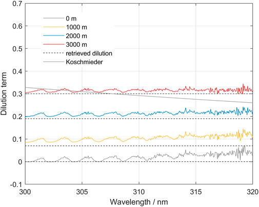
FIGURE 7. The spectral shape of the dilution function for various plume heights in the clean atmosphere, clean plume scenario. Notice that the overall shape is relatively flat over the wavelength intervals 305–315 and 310–320 used in the scattering correction method. Also notice a residual SO₂ that indicates that the effective column does not correspond exactly to the nominal column of 2,000 ppm m in this inversion. The “Koschmieder” prediction is also shown for a plume located at 3,000 m altitude.

Our results indicate that the trend in the dilution term is nearly independent of wavelength, a circumstance that is in good agreement with our proposed model. There are some structures that are correlated with the absorption of SO₂ which may be due to incomplete compensation of the term involving SO₂ in our model. This may be due to radiative transfer effects that produced an effective column that is not equal to the prescribed vertical column density used to model the different spectra. In the interpretation given by Kern et al. (2010), this could be caused by different effective pathlengths due to different absorption strength of SO₂ for different wavelengths.

Applying the ScatteringCorrection software using the lower bands 305–310/310–315 nm, we obtain the following results for retrieved column and dilution factor (Figure 8).

FIGURE 8

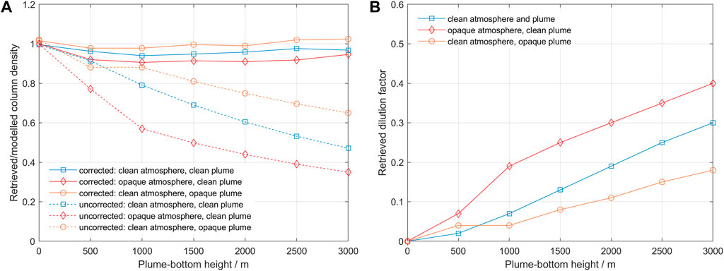
FIGURE 8. (A) Retrieved/modelled column density as a function of altitude for the three modelled cases. The results without correction are shown with dashed lines, and the results after the correction are shown with continuous lines. (B) Retrieved dilution factor as a function of altitude for the three modelled cases.

The modelling results indicate that our proposed method can deal relatively well with spectra taken under conditions of clear and opaque atmospheres and clear and opaque plumes. In all scenarios, we notice the increase of dilution factor with distance to the plume and with increase in scattering conditions below the plume. The retrieved SO₂ column densities without correction show a systematic decrease with increasing dilution, but aerosols in the plume seem to reduce the amount of dilution, possibly due to enhanced forward scattering towards the instrument. The retrieved column values after correction lie within 10% accuracy of the nominal values, being worst for the case of an opaque atmosphere and slightly better for the case of an opaque plume. We think this reflects the effect of two processes: one is that the percentage of radiation that reaches the instrument passing through the plume may be larger for an opaque plume due to higher forward scattering, and the other is that the aerosols may increase the mean path of radiation in the plume due to multiple scattering. The modelling results also show that the assumption of constant dilution within a narrow wavelength interval is reasonable.

4.2 Measurements

Next, we tested our scattering correction on real-world DOAS traverse measurements. Three different cases are shown, representing different column densities and scattering conditions: Fagradalsfjall located on Reykanaes peninsula on south Island (low columns 800 ppm m, clean air), Manam located off the northeast coast of mainland Papua New Guinea (very high columns 5,000 ppm m, high scattering), and Holuhraun located in the inland of north east Island (moderate columns 1,000–2,000 ppm m, low scattering).

4.2.1 Fagradalsfjall 2021

In March 2021, a fissure eruption occurred in Fagradalsfjall on the Reykjanes peninsula west of Reykjavik in Iceland. Figure 9 shows a traverse made around solar noon on 27 April 2021. The plume was relatively transparent, and it was easy to see through. The bottom of the plume was at about 550 m height, as determined by triangulation, and the background air was clean, but the sky was very cloudy. The initial measurement made using the standard range 310–325 nm yielded SO₂ columns around 800 ppm m. Dilution correction was applied using both the short wavelength intervals (305–310/309–314) and long wavelength intervals (309–314/314–319). Each evaluation gives similar results with corrected SO₂ columns around 1,200 ppm m, and average dilution factors of about 27%. Our corrections therefore yielded SO₂ column densities equal to 150% of the results from the standard DOAS evaluation. Note that even though both evaluation procedures yield similar results, the shorter wavelength interval gives a less noise. This demonstrates that, for low column densities, the stronger absorption in the shorter wavelength absorption bands gives a better-defined difference between the analysis windows and thus a sharper focus in the iterative correction technique.

FIGURE 9

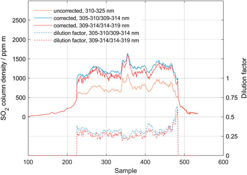
FIGURE 9. Traverse made in Fagradalsfjall on 27 April 2021. Standard evaluation (black) is compared to scattering corrected data using the lower bands (blue) and higher bands (red). Also shown are the derived dilution factors due to atmospheric scattering.

4.2.2 Manam 2019

In May 2019, a one-week international field campaign was conducted at Manam volcano in Papua New Guinea (Liu et al., 2020). The purposes of this campaign were twofold: to improve data on gas emission from this highly emitting, remotely located and little studied volcano and to demonstrate the use of drones in volcano monitoring at challenging volcanoes. These drone measurements offered unique possibilities to test our dilution correction algorithm by performing SO₂ column measurements with a MobileDOAS instrument from various altitudes below the plume (Galle et al., 2021).

On 27 May, we performed two almost simultaneous measurements (30 min apart) of the SO₂ emission rate from the volcano using two different MobileDOAS instruments, one located on the ground close to sea-level continuously pointing at zenith through the center of the plume and the other performing a drone traverse under the plume at 1 km altitude above ground. The crater is located about 1,800 m above ground and emitted a barely visible plume with a stable direction during the measurement period at an approximate altitude of 2,000 m above ground. The wind was slow, and the sky was clear. Thus, this traverse measurement is expected to show less dilution than the ground-based instrument. It is also expected that both measurements, after dilution correction, should show similar maximum SO₂ columns.

Figure 10 below shows the result of the measurement from the ground for 30 min. Here, the two longer wavelength intervals (309–314.5 and 314.5–320 nm) are used as the final columns are relatively high and the more sensitive shorter interval will contain saturated absorption bands. The original standard DOAS evaluation (blue, 1,200 ppm m) is more than tripled to about 4,400 ppm m after the scattering correction (black). The dilution factor (orange) is about 0.4. Note that the main variation in the standard measurement seems to be linked to variations in the scattering dilution factor yielding a more constant overhead SO₂ column density after the scattering correction is applied. This short-term increase in dilution factor may be caused by increased scattering below the plume due to a change in atmospheric condition or plume height, or a decrease in the fraction of light that has passed the plume. The fact that the spectrum intensity (purple, arbitrary units) increases in correlation with increased dilution indicates that the most plausible cause of this variation in dilution factor is a change in atmospheric conditions below the plume. Finally, it should be noted that the 2,000 ppm m cell measurement at the end of the measurement yields negligible dilution (0.004). This is expected as there is no atmosphere between the cell and the instrument during these cell measurements. This confirms that the stray light level in the spectrometer was negligible in this case.

FIGURE 10

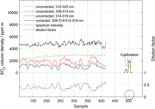
FIGURE 10. Measurement of the SO₂ vertical column at Manam on 27 May 2019, measured from a fixed position at ground. The results from measurements using the two bands 309–314 nm and 314–319 nm are shown as well as the initial and corrected columns. Also shown is the dilution factor and the spectral intensity (arbitrary units). At the end of the measurement, two cell measurements are shown with nominal values of 600 ppm m and 2,000 ppm m, respectively. Note the negligible dilution factor in this cell measurement marked with a circle. The spectrum from sample point 330 is inspected in the next figure, Figure 11.

Both the final column values and the dilution factor is relatively high in the measurement shown in Figure 10. Thus, data from this measurement can be used to test the performance of the method under such conditions. Figure 11 shows the performance of the iterative search algorithm in sample point 330. Despite the large difference between the initial SO₂ column derived by standard DOAS analysis and the dilution-corrected column, the search algorithm finds a distinct cross-over, yielding an SO₂ column density of approximately 5,200 ppm m with a dilution factor of 0.45.

FIGURE 11

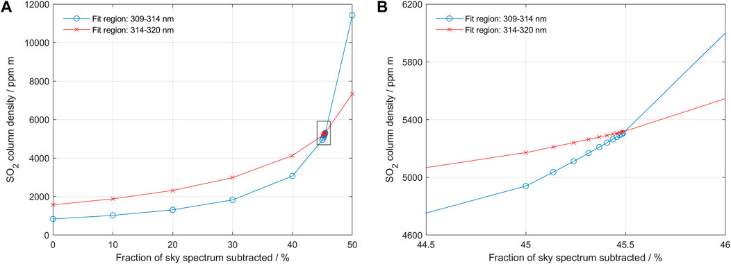
FIGURE 11. The iterative search process corresponding to data point 330 in Figure 10 above. The column value goes from 1,500 ppm m to 5,200 ppm m with a dilution factor of 0.45. Panel (B) shows a zoom-in of the region surrounded by a square in Panel (A). Note that initially the search algorithm diverges and later converges towards the final cross-over, as predicted from modelling for high columns with high dilution.

Figure 12 shows data from the MobileDOAS traverse made by drone at an altitude of 1 km above the ground. The drone traverses the plume at this altitude and then descends to 300 m altitude and starts to make a return traverse, which was not completed due to the need to land before losing power. The sampling period was set to 2 s. The maximum value of the corrected column reaches 5,000 ppm m, and the dilution factor is 0.08 at 1,000 m altitude and 0.30 at 300 m altitude (point 1,050, shown in circle). This is in good agreement with the measurements from the ground 30 min earlier, presented in Figure 10 (vertical column 5,200 ppm m, dilution factor 0.4) and confirms that the dilution caused by scattered light below the plume is the major process causing the spectroscopic imbalance between the two wavelength intervals.

FIGURE 12

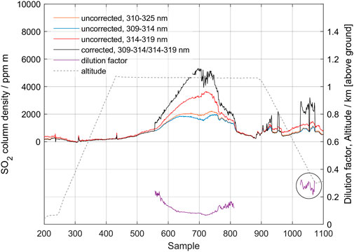
FIGURE 12. MobileDOAS measurement of the gas plume from Manam volcano, made using a drone on 27 May 2019. The drone passes under the plume at an altitude of 1 km above ground (dashed line). Results from using the two bands 309–314.5 nm and 314.5–319 nm as well as corrected column, dilution factor and altitude of the drone, as it traverses below the plume, are shown.

4.2.3 Holuhraun 2014

The 31 August 2014–27 February 2015 volcanic eruption at Holuhraun in Iceland is the strongest source of sulfur dioxide in Europe over the past 230 years, with initial sustained emission rates exceeding 100,000 td⁻¹ (Gíslason et al., 2015; Pfeffer et al., 2018). During the 6 month duration of the eruption, MobileDOAS as well as ScanningDOAS measurements were performed as part of the EU-project FUTUREVOLC. The measurements that were made close to the eruption site (5–10 km) were severely affected by atmospheric scattering, both in and around the gas plume, and showed SO₂ column densities up to 50,000 ppm m, causing severe evaluation problems. Additional measurements were conducted along the Ring Road following the Icelandic coast, at a distance 80–150 km from the eruption site. At these distances, the SO₂ columns had dropped to manageable values, and atmospheric scattering was significantly less than close to the eruption site. Figure 13 shows the results of a traverse made along the Ring Road, about 80 km north of the eruption site. Measurements were conducted around solar noon, and meteorological conditions were good with blue sky and a barely visible plume. The top of plume height was reported to be 1.6 km. A standard DOAS evaluation over the wavelength region 310–325 nm and a plume speed of 6 m s⁻¹ yielded an SO₂ emission rate of 1,379 kg s⁻¹. Figure 13 shows the result after evaluation using the standard region, 310–325 nm (blue), as well as the result after applying the scattering correction (black) and the estimated dilution. The average correction in SO₂ column gave a 60% increase in emission rate with an average dilution factor of 0.2. It should be noted that this increased emission rate to 2,200 kg s⁻¹ is even a bit higher than the underestimation due to dilution of up to 40% estimated in Pfeffer et al. (2018). Also, comparing with the radiative transfer modelling results (see Section 4.1), this dilution factor of 0.2 corresponds well with the modelled case of a clean atmosphere with a clean plume of 2,000 ppm m located at 2000 m altitude (Figure 8).

FIGURE 13

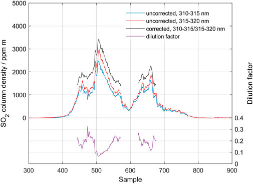
FIGURE 13. Traverse of the gas emission from Holuhraun fissure eruption in Iceland made on the Ring road on 21 September 2014.

As the duration of this traverse was relatively long (45 min), we have also evaluated this traverse using the ozone correction procedure described above. This ozone correction, however, gave only a marginal change in the evaluation result: a 3% higher average column and an identical dilution factor. The small magnitude of this effect is likely due to the fact that the traverse was made close to solar noon at 13:00 local time, so the solar zenith angle and total ozone column only changed slightly during the traverse.

5 Discussion and conclusion

This paper is a description of a novel approach to compensate for an atmospheric scattering effect that is known to significantly affect quantitative measurements of volcanic SO₂ emission rates. In its present form, the method is limited to situations when no significant multiple scattering occurs inside the volcanic plume itself, and when the absorption in the plume is strong enough to cause non-linear effects in the Beer-Lambert law (SO₂ optical depths greater than about 0.5; SO₂ column densities greater than about 400 ppm m).

Uncertainties exceeding 30% are still possible in situations where multiple scattering in optically thick volcanic plumes leads to pathlength extension (Kern et al., 2010). However, errors associated with light dilution effects which are especially pronounced when measuring a plume from distances greater than 2 km or in the presence of background aerosols or clouds and which are typically of a similar order of magnitude, are significantly reduced by our correction method. In situations where multiple scattering in the plume is not prevalent, the application of our method should eliminate atmospheric scattering as a dominant error source for SO₂ emission rate measurements, thus reducing the total error which then stems only from imperfect spectroscopy, uncertainties in measurement geometry, and potential errors in wind speed (Galle et al., 2010, see Table 3). Typical errors in SO₂ emission rates measured in good to fair conditions would then be 20%–45%, depending on the accuracy of the aforementioned other factors.

Despite these limitations, the method is believed to be useful for a first-order correction of this major error source in many measurement situations. Of special importance is that the method only uses already existing spectral information in historical data and is relatively easy to implement in existing evaluation schemes. The approach is also very logical as it directly addresses the cause of the dilution effect; it iteratively subtracts the spectrum of light that has not passed through the plume.

Here we have exclusively discussed the method for the case of mobile traverses of volcanic SO₂ plumes. However, the same method can be applied to other gases, in other wavelength intervals, and for other measurement geometries, given that the conditions stated above are fulfilled.

In particular, the use of this method to correct for scattering effects in scanning DOAS measurements of volcanic SO₂ emissions is of high interest, but further modelling is required. During the past two decades, these instruments have been installed on many volcanoes, and thus large amounts of data are available, collected under varying atmospheric and volcanic conditions. For example, the NOVAC (Network for Observation of Volcanic and Atmospheric Change) [Galle et al., 2010; Arellano et al., 2021; www.novac-community.org] today has an archive containing gas measurements from more than 40 volcanoes collected since 2005. A re-processing of this archive, containing several millions of emission rate measurements, using the suggested algorithm is expected to give a detailed insight in the magnitude of this spectral dilution effect. This then opens the possibility to estimate the effect of dilution also in historical data made by COSPEC or DOAS instruments, where spectra are not available. As most estimates of volcanic emissions of species other than SO₂ are based on scaling X/SO₂ ratios to SO₂ emission rates, such a reprocessing would allow revision of emission estimates for these species as well. It should be noted, however, that the algorithm suggested here is based on the assumption that the clean air spectrum used in the iterative subtraction, and the true dilution spectrum caused by scattering below the plume, have similar shape over the two wavelength intervals used in the analysis. This condition is realistic for many cases when using MobileDOAS zenith looking measurements made close in time, while it may be less obvious for ScanDOAS measurements with varying looking directions between sky and plume measurements. Thus, a detailed analysis of the applicability of the suggested method for ScanDOAS measurements requires further investigation with modelling and measurements and is beyond the scope of this paper.

Data availability statement

The raw data and data presented in the figures are made available in the Supplementary Material.

Author contributions

BG and SA contributed to all parts of the paper. MJ wrote the program “Scatteringcorrection.exe” used to facilitate evaluation of the raw data according to the suggested method. CK and SA worked with the modelling of synthetic spectra and MP provided the data from Fagradalsfjall on Iceland. All authors contributed to the article and approved the submitted version.

Funding

The work at Chalmers University of Technology was funded by the FORMAS project “Development and Implementation of an Algorithm for Improved Volcanic Gas Emission Monitoring, Geophysical Research and Volcano Risk Assessment,” the project “Aerial Observations of Volcanic Emissions from Unmanned Aerial Systems (UAS)” funded by the Alfred P. Sloan foundation, and a grant (149/18) from the Swedish National Space Agency.

Acknowledgments

We acknowledge the logistical and scientific support by Rabaul Volcanological Observatory (RVO), as well as the generous hospitality given by the Manam communities of Baliau and Manam during our field work in Papua New Guinea. The authors would like to thank Matt Varnam and the two journal reviewers for providing thoughtful comments on this manuscript. Any use of trade, product, or firm names is for descriptive purposes only and does not imply endorsement by the U.S. Government.

Conflict of interest

The authors declare that the research was conducted in the absence of any commercial or financial relationships that could be construed as a potential conflict of interest.

Publisher’s note

All claims expressed in this article are solely those of the authors and do not necessarily represent those of their affiliated organizations, or those of the publisher, the editors and the reviewers. Any product that may be evaluated in this article, or claim that may be made by its manufacturer, is not guaranteed or endorsed by the publisher.

Supplementary material

The Supplementary Material for this article can be found online at: https://www.frontiersin.org/articles/10.3389/feart.2023.1088768/full#supplementary-material

References

Aiuppa, A., Bitetto, M., Donne, D. D., Paolo, F., Monica, L., Tamburello, G., et al. (2021). Volcanic CO₂ tracks the incubation period of basaltic paroxysms. Sci. Adv. 7, eabh0191. doi:10.1126/sciadv.abh0191

PubMed Abstract | CrossRef Full Text | Google Scholar

Aiuppa, A., Moretti, R., Federico, C., Giudice, G., Gurrieri, S., Liuzzo, M., et al. (2007). Forecasting Etna eruptions by real-time observation of volcanic gas composition. Geology 35, 1115. doi:10.1130/G24149A.1

CrossRef Full Text | Google Scholar

Arellano, S., Galle, B., Apaza, F., Avard, G., Barrington, C., Bobrowski, N., et al. (2021). Synoptic analysis of a decade of daily measurements of SO₂ emission in the troposphere from volcanoes of the global ground-based Network for Observation of Volcanic and Atmospheric Change. Earth Syst. Sci. Data 13, 1167–1188. doi:10.5194/essd-13-1167-2021

CrossRef Full Text | Google Scholar

Bogumil, K., Orphal, J., Homann, T., Voigt, S., Spietz, P., Fleischmann, O., et al. (2003). Measurements of molecular absorption spectra with the SCIAMACHY pre-flight model: Instrument characterization and reference data for atmospheric remote-sensing in the 230–2380 nm region. J. Photochem. Photobiol. Chem. A 157, 167–184. doi:10.1016/S1010-6030(03)00062-5

CrossRef Full Text | Google Scholar

Burton, M., Allard, P., Mure, F., and La Spina, A. (2007). Magmatic gas composition reveals the source depth of slug-driven strombolian explosive activity. Science 317, 227–230. doi:10.1126/science.1141900

PubMed Abstract | CrossRef Full Text | Google Scholar

Campion, R., Delgado Granados, H., and Mori, T. (2015). Image-based correction of the light dilution effect for SO₂ camera measurements. J. Volcanol. Geotherm. Res. 300, 48–57. doi:10.1016/j.jvolgeores.2015.01.004

CrossRef Full Text | Google Scholar

de Moor, J. M., Aiuppa, A., Avard, G., Wehrmann, H., Dunbar, N., Muller, C., et al. (2016a). Turmoil at Turrialba Volcano (Costa Rica): Degassing and eruptive processes inferred from high-frequency gas monitoring. J. Geophys. Res. Solid Earth 121, 5761–5775. doi:10.1002/2016JB013150

PubMed Abstract | CrossRef Full Text | Google Scholar

de Moor, J. M., Aiuppa, A., Pacheco, J., Avard, G., Kern, C., Liuzzo, M., et al. (2016b). Short-period volcanic gas precursors to phreatic eruptions: Insights from Poás Volcano, Costa Rica. Earth Planet. Sci. Lett. 442, 218–227. doi:10.1016/j.epsl.2016.02.056

CrossRef Full Text | Google Scholar

Deutschmann, T., Beirle, S., Frieß, U., Grzegorski, M., Kern, C., Kritten, L., et al. (2011). The Monte Carlo atmospheric radiative transfer model McArtim: Introduction and validation of jacobians and 3D features. J. Quantitative Spectrosc. Radiat. Transf. 112 (6), 1119–1137. doi:10.1016/j.jqsrt.2010.12.009

CrossRef Full Text | Google Scholar

Deutschmann, T., Beirle, S., Frieß, U., Grzegorski, M., Kern, C., Kritten, L., et al. (2011). The Monte Carlo atmospheric radiative transfer model McArtim: Introduction and validation of jacobians and 3D features. J. Quantitative Spectrosc. Radiat. Transf. 112 (6), 1119–1137. doi:10.1016/j.jqsrt.2010.12.009

CrossRef Full Text | Google Scholar

Edmonds, M., Herd, R. A., Galle, B., and Oppenheimer, C. (2003). Automated, high time resolution measurements of SO₂ flux at Soufrière Hills Volcano, Montserrat. Bull. Volcanol. 65 (8), 578–586. doi:10.1007/s00445-003-0286-x

CrossRef Full Text | Google Scholar

Esse, B., Burton, M., Varnam, M., Kazahaya, R., and Salerno, G. (2020). iFit: A simple method for measuring volcanic SO₂ without a measured Fraunhofer reference spectrum. J. Volcanol. Geotherm. Res. 402, 107000. doi:10.1016/j.jvolgeores.2020.107000

CrossRef Full Text | Google Scholar

Fickel, M., and Delgado Granados, H. (2017). On the use of different spectral windows in DOAS evaluations: Effects on the estimation of SO₂ emission rate and mixing ratios during strong emission of Popocatépetl volcano. Chem. Geol. 462, 67–73. doi:10.1016/j.chemgeo.2017.05.001

CrossRef Full Text | Google Scholar

Galle, B., Arellano, S., Bobrowski, N., Conde, V., Fischer, T. P., Gerdes, G., et al. (2021). A multi-purpose, multi-rotor drone system for long-range and high-altitude volcanic gas plume measurements. Atmos. Meas. Tech. 14 (1–23), 4255–4277. doi:10.5194/amt-14-4255-2021

CrossRef Full Text | Google Scholar

Galle, B., Johansson, M., Rivera, C., Zhang, Y., Kihlman, M., Kern, C., et al. (2010). Network for observation of volcanic and atmospheric change (NOVAC)—a global network for volcanic gas monitoring: Network layout and instrument description. J. Geophys. Res. 115, D05304. doi:10.1029/2009JD011823

CrossRef Full Text | Google Scholar

Galle, B., Oppenheimer, C., Geyer, A., McGonigle, A., Edmonds, M., and Horrocks, L. (2003). A miniaturised ultraviolet spectrometer for remote sensing of SO₂ fluxes: A new tool for volcano surveillance. J. Volcanol. Geotherm. Res. 119, 241–254. doi:10.1016/S0377-0273(02)00356-6

CrossRef Full Text | Google Scholar

Gerlach, T. M. (2004). Volcanic sources of tropospheric ozone-depleting trace gases. Geochem. Geophys. Geosystems 5, 1–16. doi:10.1029/2004GC000747

CrossRef Full Text | Google Scholar

Giggenbach, W. F. (1996). “Chemical composition of volcanic gases,” in Monitoring and mitigation of volcano hazards. Editors R. Scarpa, and R. Tilling (Berlin, Heidelberg: Springer), 221–256. doi:10.1007/978-3-642-80087-0_7

CrossRef Full Text | Google Scholar

Gíslason, S. R., Stefánsdóttir, G., Pfeffer, M. A., Barsotti, S., Jóhannsson, T., Galeczka, I., et al. (2015). Next article >> << Previous article Environmental pressure from the 2014–15 eruption of Bárðarbunga volcano, Iceland. Geochem. Perspect. Lett. 1, 84–93. doi:10.7185/geochemlet.1509

CrossRef Full Text | Google Scholar

Johansson, M. (2009). Application of passive DOAS for studies of megacity air pollution and volcanic gas emissions. PhD thesis, Chalmers University of Technology, Gothenburg, 64.

Google Scholar

Johansson, M., Galle, B., Yu, T., Tang, L., Chen, D., Li, H., et al. (2008). Quantification of total emission of air pollutants from Beijing using mobile mini-DOAS. Atmos. Environ. 42, 6926–6933. doi:10.1016/j.atmosenv.2008.05.025

CrossRef Full Text | Google Scholar

Kern, C., Aiuppa, A., and de Moor, J. M. (2022). A golden era for volcanic gas geochemistry? Bull. Volcanol. 84, 43–11. doi:10.1007/s00445-022-01556-6

CrossRef Full Text | Google Scholar

Kern, C., Deutschmann, T., Vogel, L., Wöhrbach, M., Wagner, T., and Platt, U. (2010). Radiative transfer corrections for accurate spectroscopic measurements of volcanic gas emissions. Bull. Volcanol. 72 (2), 233–247. doi:10.1007/s00445-009-0313-7

CrossRef Full Text | Google Scholar

Kern, C., Deutschmann, T., Werner, C., Sutton, A. J., Elias, T., and Kelly, P. J. (2012). Improving the accuracy of SO₂ column densities and emission rates obtained from upward-looking UV-spectroscopic measurements of volcanic plumes by taking realistic radiative transfer into account. J. Geophys. Res. Atmos. 117 (D20), D20302. doi:10.1029/2012JD017936

CrossRef Full Text | Google Scholar

Kern, C. (2019). MatArtim: A matlab scripting interface for the McArtim radiative transfer model. (unpublished) version 1.1.

Google Scholar

Koschmieder, H. (1938). Luftlicht und Sichtweite. Naturwissenschaften 26, 521–528. doi:10.1007/BF01774261

CrossRef Full Text | Google Scholar

Kunrat, S., Kern, C., Alfianti, H., and Lerner, A. H. (2022). Forecasting explosions at Sinabung Volcano, Indonesia, based on SO₂ emission rates. Front. Earth Sci. 10, 976928. doi:10.3389/feart.2022.976928

CrossRef Full Text | Google Scholar

Liu, E. J., Aiuppa, A., Alan, A., Arellano, S., Bitetto, M., Bobrowski, N., et al. (2020). Aerial strategies advance volcanic gas measurements at inaccessible, strongly degassing volcanoes. Sci. Adv. 6 (44), eabb9103. doi:10.1126/sciadv.abb9103

PubMed Abstract | CrossRef Full Text | Google Scholar

Millàn, M. M. (1980). Remote sensing of air pollutants. A study of some atmospheric scattering effects. Atmos. Environ. 14 (11), 1241–1253. doi:10.1016/0004-6981(80)90226-7

CrossRef Full Text | Google Scholar

Moffat, A. J., and Millàn, M. M. (1971). The applications of optical correlation techniques to the remote sensing of SO₂ plumes using sky light. Atmos. Environ., 5 (8), 677–690. doi:10.1016/0004-6981(71)90125-9

PubMed Abstract | CrossRef Full Text | Google Scholar

Mori, T., Kazahaya, K., Ohwada, M., Hirabayashi, J., and Yoshikawa, S. (2006). Effect of UV scattering on SO₂ emission rate measurements. Geophys. Res. Lett. 33 (17), L17315. doi:10.1029/2006GL026285

CrossRef Full Text | Google Scholar

Oppenheimer, C., Fischer, T. P., and Scaillet, B. (2014). “Volcanic degassing: Process and impact,” in Treatise on geochemistry. Editors H. Holland, and K. Turekian Second Edition (Elsevier), 111–179. doi:10.1016/B978-0-08-095975-7.00304-1

CrossRef Full Text | Google Scholar

Pfeffer, M. A., Bergsson, B., Barsotti, S., Stefánsdóttir, G., Galle, B., Arellano, S., et al. (2018). Ground-based measurements of the 2014–2015 Holuhraun volcanic cloud (Iceland). Geosciences 8, 29. doi:10.3390/geosciences8010029

CrossRef Full Text | Google Scholar

Platt, U., Lübcke, P., Kuhn, J., Bobrowski, N., Prata, F., Burton, M., et al. (2015). Quantitative imaging of volcanic plumes–Results, needs, and future trends. J. Volcanol. Geotherm. Res. 300, 7–21. doi:10.1016/j.jvolgeores.2014.10.006

CrossRef Full Text | Google Scholar

Platt, U., and Stutz, J. (2008). Differential optical absorption spectroscopy principles and applications. in Physics of Earth and Space environments. Springer, 597. doi:10.1007/978-3-540-75776-4

CrossRef Full Text | Google Scholar

Sparks, R. S. J., Biggs, J., and Neuberg, J. W. (2012). Monitoring volcanoes. Science 335, 1310–1311. doi:10.1126/science.1219485

PubMed Abstract | CrossRef Full Text | Google Scholar

Varnam, M., Burton, M., Esse, B., Kazahaya, R., Salerno, G., Caltabiano, T., et al. (2020). Quantifying light dilution in ultraviolet spectroscopic measurements of volcanic SO₂ using dual-band modeling. Front. Earth Sci. 8, 528753. doi:10.3389/feart.2020.528753

CrossRef Full Text | Google Scholar

Vogel, L., Galle, B., Kern, C., Delgado Granados, H., Conde, V., Norman, P., et al. (2011). Early in-flight detection of SO₂ via differential optical absorption spectroscopy: A feasible aviation safety measure to prevent potential encounters with volcanic plumes. Atmos. Meas. Tech. 4, 1785–1804. doi:10.5194/amt-4-1785-2011

CrossRef Full Text | Google Scholar