Climatic and seismic data-driven deep learning model for earthquake magnitude prediction

The effects of global warming are felt not only in the Earth’s climate but also in the geology of the planet. Modest variations in stress and pore-fluid pressure brought on by temperature variations, precipitation, air pressure, and snow coverage are hypothesized to influence seismicity on local and regional scales. Earthquakes can be anticipated by intelligently evaluating historical climatic datasets and earthquake catalogs that have been collected all over the world. This study attempts to predict the magnitude of the next probable earthquake by evaluating climate data along with eight mathematically calculated seismic parameters. Global temperature has been selected as the only climatic variable for this research, as it substantially affects the planet’s ecosystem and civilization. Three popular deep neural network models, namely, long short-term memory (LSTM), bidirectional long short-term memory (Bi-LSTM), and transformer models, were used to predict the magnitude of the next earthquakes in three seismic regions: Japan, Indonesia, and the Hindu-Kush Karakoram Himalayan (HKKH) region. Several well-known metrics, such as the mean absolute error (MAE), mean squared error (MSE), log-cosh loss, and mean squared logarithmic error (MSLE), have been used to analyse these models. All models eventually settle on a small value for these cost functions, demonstrating the accuracy of these models in predicting earthquake magnitudes. These approaches produce significant and encouraging results when used to predict earthquake magnitude at diverse places, opening the way for the ultimate robust prediction mechanism that has not yet been created.

1 Introduction

Climate change is defined as an alteration in the climate as measured by statistical parameters such as the global mean surface temperature. The term “climate” here refers to the long-term pattern of meteorological conditions that has prevailed over the past three decades. Climate is made up of many factors, such as temperature, humidity, precipitation, air pressure, wind speed, evaporation, cloud cover, condensation, radiation, and evapotranspiration. The climate and temperature of Earth are increasingly influenced by both natural forces, such as variations in solar radiation, and human activities, such as the burning of fossil fuels and deforestation. Changes in the relative amounts of solar radiation and the Earth’s emitted infrared radiation are the root causes of climate change. Observations indicate that the global temperature rose by 1.4°F (0.78°C) between 1900 and 2005 (Singh and Singh, 2012). Several additional climatic events, such as extreme heat waves, glacial melting, sea ice loss, soaring sea levels, frequent heavy rains and ocean acidification, are intimately related to global warming. The effects of global warming are not restricted to climate change alone; the entire planet is grappling with the effects of an energy imbalance. This imbalanced energy might manifest as isostatic rebound, a volcanic explosion, or an earthquake. Human activities have been the primary source of the planet’s warming during the past few decades (Intergovernmental Panel on Climate Change, 2014).

According to records, there has been a significant rise in temperature in the Northern Hemisphere over the past 1,400 years (Pachauri et al., 2014). The previous three decades have seen the bulk of this warming. Figure 1 displays the annual variance in global surface temperature relative to the 20th century average. Climate change has led to an increase in sea level, a decrease in ice cover, and exacerbation of severe meteorological conditions, such as intensified tropical cyclones and severe droughts. Increased emissions of greenhouse gases from power plants, industry, and automobiles exacerbate this warming, which impacts not only the Earth’s climate but also the geology of the planet (Singh and Singh, 2012). This growth primarily originated from the burning of fossil fuels and growing urbanization. Additionally, enhanced climatic forcing perpetuates this warming owing to rising quantities of greenhouse gases (McCormick et al., 2007).

FIGURE 1

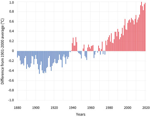
FIGURE 1. Global surface temperature (yearly) compared to the average temperature of the 20th century, Duration 1880–2020. Years that were colder than normal are shown by blue bars, while years that were warmer than average are represented by red bars. Source: Climate.gov (NOAA).

Climate change has sparked widespread concern among scientists and policymakers in recent years. As the Earth warms, Greenland and polar regions' ice sheets and mountain glaciers melt, lessening the glacial load on the crust. The crust relaxes and rebounds as these glaciers melt. Glacial melting has boosted the flow of glacial rivers. There has been a massive outflow of water into the ocean as a result, which might disrupt the delicate equilibrium of plate tectonics on a global scale (Glick, 2011; Mara and Vlad, 2013). Solid Earth is unloaded due to the decay of glacial ice sheets and caps as shown in Figure 2. This unloading can cause crustal deformation and mantle expansion. (Smiraglia et al., 2007; Pagli and Sigmundsson, 2008). The crust progressively rises owing to isostatic rebound because of erosion or glacial melting, causing crustal deformations and tectonic motion (Larsen et al., 2005).

FIGURE 2

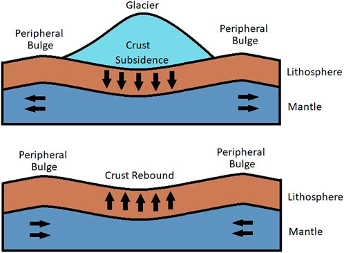
FIGURE 2. Effect of Glacier Melt on Earth’s crust.

According to satellite data collected worldwide, glacier mass is decreasing in the high mountain regions of Alaska, coastal Greenland, arctic Canada, the southern Andes, and Asia. Furthermore, significant amounts of water are being discharged into the oceans (Kaser et al., 2006; Meier et al., 2007; Gardner et al., 2013; Abdullah et al., 2020). Figure 3 depicts a global summary of the World Glacier Monitoring Service’s findings on the mass changes of selected glaciers (Global Glacier State – World Glacier Monitoring Service, 2021). This figure shows the changes in glacier mass over time, as measured in millimetres of equivalent water.

FIGURE 3

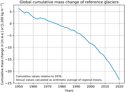
FIGURE 3. Variation in the cumulative mass of reference glaciers. The value is expressed as a meter water equivalent (mwe) compared to 1976. Source: World Glacier Monitoring Service (WGMS).

Since the Industrial Revolution, it has been largely believed that global warming has played a major role in rising global sea levels (Church and White, 2011). Furthermore, it is assumed that the decay of glacier ice and ocean thermal expansion played a significant role in global sea-level rise during the 20th century (Church and White, 2011).

Figure 4 shows the rise in sea level since 1993 (black line). Thermal expansion (red line) and increased water mostly owing to melting glaciers (blue line) are just two of the many factors for which exact estimates are available. As shown in Figure 5, the subsidence of the crust is initiated by the additional weight imposed by global sea-level rise. In addition, subsidence of the crust can promote plate tectonics to counterbalance the increased stress caused by the added seawater.

FIGURE 4

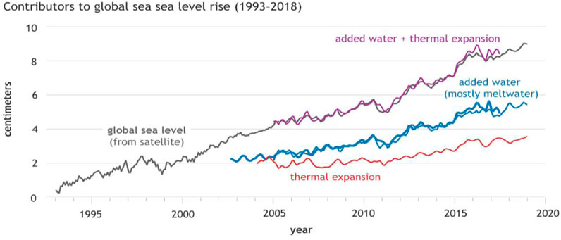
FIGURE 4. Rise in global sea levels as seen through satellite altimeters, Period: 1993–2018. Source: NOAA.

FIGURE 5

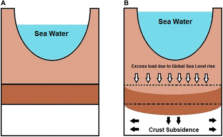
FIGURE 5. Land subsidence caused by additional seawater.

Earthquakes occur when the Earth’s tectonic plates move as a result of a sudden and large release of internal energy. Earthquakes are one of the most devastating natural disasters. Earthquakes frequently hit without notice, giving people little time to make preparations. In addition, earthquakes frequently cause other natural disasters, such as surface fault rupture (Bray, 2001), tsunamis (Jain, Virmani, and Abraham, 2019), snow slides (Podolskiy et al., 2010), landslides (KEEFER, 1984), soil liquefication (Verdugo and González, 2015), and fires (Cassidy, 2013), which exacerbate the crisis. Devastating earthquakes cause deaths (Ambraseys and Melvilleand, 1983), massive infrastructure damage (Bilham, 2009), societal defeat, and a rapid economic downturn (So and Platt, 2014). In the last two decades, earthquakes have caused more than half of all natural disaster-related fatalities (Bartels and VanRooyen, 2012). The devastating effects of significant earthquakes can be lessened with timely and accurate predictions that allow for the adoption of preventative measures. A reliable forecast indicates an earthquake’s location, time, and magnitude. These predictions can save many lives and resources. Although several strategies employing diverse input factors have been offered, such accurate forecasts are uncommon in past research (Otari and Kulkarni, 2012). Researchers in seismology and related disciplines have attempted to identify earthquake precursors. Since the end of the 19th century, these unusual phenomena have typically occurred before earthquakes. According to various studies, earthquakes can be predicted by observations of numerous precursors, such as temperature increases (Zandonella, 2001; Sadhukhan et al., 2021b; Sadhukhan et al., 2021c; Maji et al., 2021), ionospheric analysis (Pulinets, 2004), animal behaviour (Fidani, 2013; Cao and Huang, 2018), hydrogeological and gas geochemical analysis (Hartmann and Levy, 2005) and radon gas emissions (Petraki et al., 2015).

The majority of earthquake prediction techniques rely on the existence of particular precursors (Ikram and Qamar, 2014). However, in reality, these precursors often do not materialise with subsequent seismic occurrences or are hard to recognize, so these approaches may not always produce desirable outcomes (Wang et al., 2020). As the precursors do not necessarily occur before every earthquake, it is exceedingly difficult to generalize and standardize these prediction systems. This has led to the proposal of novel methods for future earthquake prediction (Tiampo and Shcherbakov, 2012).

Earthquake prediction can be of two types: long-term and short-term. Predicting earthquakes within the next several days, weeks, or months is a very challenging task requiring a great deal of data and analysis. As a result, it ought to be reliable and accurate, with a minimum of false positives (Goswami et al., 2018). Short-term forecasts are commonly used to evacuate a region ahead of an earthquake. Long-term prediction is based on the timing and location of past earthquakes. Therefore, the existing tectonic context, historical data, and geographical information are evaluated to determine where and how frequently earthquakes occur. However, it can help define building code standards and develop emergency response plans.

Earthquake prediction is a vital subject in seismology since successful prediction can save lives, property, and infrastructure. Although earthquakes appear to be active and spontaneous, they often fail to provide favourable outcomes. Numerous technologies, such as mathematical analysis, artificial intelligence, and machine learning algorithms, have been proposed to address this issue. Many different approaches have been used in recent theoretical and practical investigations of earthquake prediction. Air ionization, radon migration, latent heat release, variation in surface temperature, air pressure, relative humidity, cloud formation, coupling with precipitation anomalies, radio wave propagation, ionosphere and magnetosphere effects are all climate-associated variables that have been identified as potential precursors to future earthquakes (Daneshvar and Freund, 2017).

Earthquake prediction models perform admirably for earthquakes of moderate magnitude; however, the results obtained with large shocks are disappointing. Large earthquakes cause the most damage and concern. As high-magnitude earthquakes are uncommon, it is difficult to predict them due to a lack of appropriate evidence. After a decade of effort, the seismology community has been unable to devise a system for earthquake prediction. Predictions of earthquakes continue to be impossible due to the inadequacy of current technology to monitor stresses and pressure changes more precisely through scientific equipment positioned beneath the crust; hence, considerable seismic data are always limited. Due to a lack of multidisciplinary collaboration between seismology and computer science departments to accurately predict and quantify earthquake occurrences, earthquake prediction has remained a challenging endeavour to date. Due to the extremely non-linear and complex geophysical processes that create earthquakes, no mathematical or empirical relationship exists between any physically recordable parameter and the timing, magnitude, or location of a future earthquake (Panakkat and Adeli, 2007).

The following is the outline of the study: The relevant prior research is outlined in Section 2. The research’s data and methodology are described in Section 3, and its analytical methods are presented in Section 4. The deep neural network models employed in this research are outlined in Section 5, and their results are discussed in Section 6. Finally, Section 7 draws the necessary conclusion.

2 Related work

There is increasing evidence in the scientific community suggesting that climate change also contributes to geological occurrences such as tremors, tsunamis, and volcanic eruptions. In recent years, numerous researchers throughout the world have been striving to verify the effect of climate change on seismicity. The occurrence of earthquakes is assumed to be a random and extremely non-linear process, and no model exists that can predict the exact time, position, and magnitude of earthquakes. Numerous studies have been undertaken on earthquake occurrences and forecasts, yielding a variety of conclusions regarding the subject.

Several studies have revealed significant irregularities in climatic factors before large earthquakes. Satellite thermal imaging has revealed long and short-term temperature abnormalities preceding major earthquakes (Tronin et al., 2002; Pulinets et al., 2006; Jiao et al., 2018; Pavlidou et al., 2019). These transient abnormalities might vary by 2°C–4°C between four to 20 days before an earthquake and gradually disappear thereafter (Ouzounov et al., 2007). Some unexpected abnormalities were found above clouds in the atmosphere and the lithosphere (Sasmal et al., 2021). A variety of factors, such as changes in the crust’s geophysics, contribute to the occurrence of seismic foreshocks. The lithosphere-atmosphere-ionospheric coupling (LAIC) model can be used to defend against these irregularities (Pulinets and Ouzounov, 2011; Carbone et al., 2021).

Preliminary research was conducted on the aberrant variations in the enhanced surface-latent heat flux and water vapour anomaly before the Colima and Gujarat earthquakes (Dey and Singh, 2003; Dey et al., 2004). Many different climate factors and processes may influence seismic activity. Changes in many critical climatic variables often precede severe earthquakes. These include surface latent heat flow, precipitation, wind speed, cloudiness and vertical air flow (Mansouri Daneshvar and Freund, 2021). At many regional and temporal scales, comprehensive studies utilizing various time intervals and spatial resolutions indicate increased precipitation preceding large seismic events. Therefore, a significant positive relationship seems to be present between seismicity and precipitation prior to the major shocks (R = 0.711).

Consequently, seismic events foretell climatic abnormalities, increase precipitation, and create cyclones. Heavy rainfall across the seismic region within 5 days after a large earthquake was shown to be substantially correlated with such events (Zhao et al., 2021). Approximately 74.9% of earthquakes in China were followed by epicentral rainfall, while 86.6% of earthquakes were accompanied by seismic area rainfall. Rainfall is more prevalent in earthquake zones than in the 30-year climatic trends, and earthquakes predominate during the monsoon season (Zhao et al., 2021).

Increased rainfall has been seen in Iran and the neighbouring middle east region just before major earthquakes between 2002 and 2013 (Mansouri Daneshvar et al., 2014). The researchers investigated the geographical correlations between seismic occurrence and meteorological changes by grouping 39 significant earthquakes into eight seismological areas. They found moderate and high correlations (R²) between the preceding precipitation and the magnitudes and hypocentre depths of large earthquakes. Further studies indicated that rainfall has the capacity to anticipate earthquake sequences beginning at least three and a half months in advance. The estimated lagged correlation demonstrates a positive relationship between precipitation and subsequent earthquake occurrence days, with lags ranging from 3 to 103 days (Mansouri Daneshvar et al., 2021).

Even though earthquakes lead to all types of climatic anomalies, rainfall statistics are largely significant factors in estimating the place and magnitude of possible tremors. Extremely dry conditions (drought) often precede major earthquakes, and then one or more years of above-average precipitation are usually followed by tremors (Huang et al., 1979). Fluctuations in surface heat flow around the epicentre zone have been related to enhanced thermal energy at the Earth’s surface, which is thought to be the cause of this anomalous precipitation. The increase in sensible heat flow aids the process of evapotranspiration, which produces atmospheric water vapour. This might lead to the formation of clouds and abnormal precipitation. Researchers have shown that semi-stationary linear cloud development is also associated with increased seismicity (Guangmeng and Jie, 2013; Thomas et al., 2015). Abnormal rainstorms over the epicentral area have also been documented prior to major earthquakes (Mullayarov et al., 2012; Daneshvar and Freund, 2017).

Some intriguing studies explicitly establish a correlation between the incidence of earthquakes and the increase in surface temperature. Begley (2006) claims that earthquakes occur when nucleation processes release significant amounts of stored energy along the fault plane. Reduced stress on the crust as a response to glacial decay generates “isostatic rebound,” which eventually results in fault resurfacing and increased seismicity. Numerous researchers have attempted to establish the connection between rising temperatures and seismic activity (Usman and Amir, 2009; Usman et al., 2011; Usman, 2016). The study region included several glaciers. Rising global temperatures caused these glaciers to melt, relieving pressure on the Earth below. As a result, seismic activity may have increased, causing the Earth to rebound. Most earthquakes on the Richter scale were between 3.0 and 3.9, and seismic activity continued to grow with rising temperatures. Further research showed that an increase in temperature is associated with an increase in the number of shallow earthquakes (between 0 and 80 km). A plausible correlation between rising earthquake activity and climate change was proposed by Mara and Vlad (2013). Glacial ice sheets cover 10% of Earth’s entire crustal area; hence, any changes in their extent due to glacier decay would have significant implications on the planet’s tectonic stability.

The rapid depletion of ice caps is another obvious effect of global warming. McGuire (2013)’s study suggests that the decline in ice sheets can also produce earthquakes. He asserted that a rise in global temperature over several decades triggered the melting of enormous, thick ice sheets, enabling the crust to bounce back. As global sea levels continue to rise indefinitely, load-related crust deformation at ocean basin margins may ultimately “unclamp” coastal faults. There is substantial evidence of a major relationship between climatic change and earthquakes during the transition from the previous ice age, notably in North America and Scandinavia. The environment of the Northern Hemisphere, notably Alaska, is significantly impacted by climate change and global warming (Hinzman et al., 2005).

Sadhukhan et al. (2021c) studied the relationships between earthquake magnitudes and variations in global temperature by applying signal processing methods. Semblance analysis was used to verify the association between these two dynamics. The causality test reveals that the two dynamics are strongly connected, indicating that one may be expected given the historical data of the other. The authors then employed a variety of statistical signal processing techniques to explore the multifractal, non-linear, and chaotic nature of two dynamics: earthquake magnitude and global temperature variations (Sadhukhan et al., 2021b). A correlation study determined the degree of correlation between global earthquake frequency and global temperature changes (Maji et al., 2021). Additionally, RNN-based deep learning models are used to verify the relationship between climate change and seismicity (Sadhukhan et al., 2021a).

Using statistical methods such as correlation and regression analysis, Masih (2018) investigated the correlation between climate change and the frequency of earthquakes. Furthermore, the study asserts that climate change due to global warming triggers the decline of glacial ice sheets, depressurization of the underlying rocks and reactivation of faults, thereby classifying the region as seismically active with frequent earthquakes. Molchanov (2010) used correlation analysis to explore the relationship between climatic change (temperature) and crustal seismicity. He found that fluctuations in temperature and seismic activity exhibited comparable tendencies. Evidence was presented by Swindles et al. (2017) that glacial extent, driven by climate, impacted the frequency of seismic events and volcanic activity in Iceland throughout millennia.

Based on the preceding discussions, an attempt has been made to predict the magnitude of the next probable earthquake by evaluating the climate data along with eight mathematically calculated seismic parameters. Three widely used deep neural network models, namely, long short-term memory (LSTM), bidirectional long-term memory (Bi-LSTM), and transformer models, were used to predict the magnitude of future earthquakes in a given seismic region using climate data and eight seismic parameters calculated from a predefined number of past significant seismic events with a predefined threshold magnitude or greater. Since global temperature has such a profound effect on the planet’s ecosystems and civilization, it has been chosen as the single climatic variable for this analysis. The geological structure and features are the same throughout the study area. This makes it possible to make accurate models of the relationship between global temperature and mathematically derived seismic parameters for predicting the magnitude of the next earthquake. These models can accurately predict the magnitude of the next approaching earthquake, which is the significance of this work. In addition, they have a high-performance metric for accurately forecasting earthquake magnitude ranges.

3 Data and methods

Deep learning-based earthquake prediction research has been carried out in Indonesia, Japan and the Hindu-Kush Karakoram Himalaya (HKKH) region. Each of these places has a high frequency of earthquakes, making them suitable for earthquake prediction research. The underlying dataset for this research is a temporal series of historical seismicity for the indicated locations. Global temperature anomaly data extracted from the global land and ocean temperature anomaly dataset maintained by the National Oceanic and Atmospheric Administration (NOAA) of the United States Department of Commerce has been used as the experimental dataset (https://www.ncei.noaa.gov/access/monitoring/climate-at-a-glance/global/time-series). Additionally, historical seismicity data from the United States Geological Survey (USGS), which is publicly available at https://earthquake.usgs.gov/earthquakes/search/, have also been used for this investigation. This study explored both datasets from January 1921 to December 2020. The coordinate boundaries of these regions are shown in Table 1, and their catalogs are evaluated to calculate the magnitude of completeness. The minimum magnitude below which an earthquake catalogue is deemed incomplete is known as the catalogue’s magnitude of completeness $\left(M_c\right).$ Among the well-known catalog-based approaches for calculating $M_c$, fitting a Gutenberg-Richter model to the observed frequency-magnitude distribution has received much attention in recent works (Wiemer, 2000; Pavlenko and Zavyalov, 2022; Yuliastuti et al., 2022). This method has a major limitation in dealing with a small number of events in a catalog. In this study, the Gutenberg-Richter law of seismic magnitude distribution has been deployed, as all the seismic catalogues used have a wide time frame and a broad experimental study region for capturing enormous seismic events to compute $M_c$.

TABLE 1

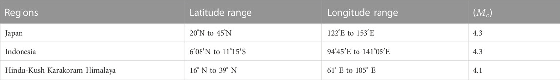
TABLE 1. Magnitude of completeness of earthquake catalogs and range of coordinate bounds considered for different regions.

This method sorts earthquakes into “bins” based on the number of occurrences with magnitudes exceeding a predetermined threshold. The count for each bin is then displayed on a similar logarithmic scale. If they were statistically accurate, the data would form a straight line. Although it is nearly impossible to obtain statistically perfect datasets, we can estimate $M_c$ using this relationship. When a straight line is fitted to the data, the point where the data deviate from the line indicates the level of completeness. Figures 6A–C depict the cumulative count of earthquakes that occurred by decreasing magnitude on a logarithmic scale for Indonesia, Japan and the HKKH region, respectively. Table 1 summarizes the magnitude of completeness computed for these regions.

FIGURE 6

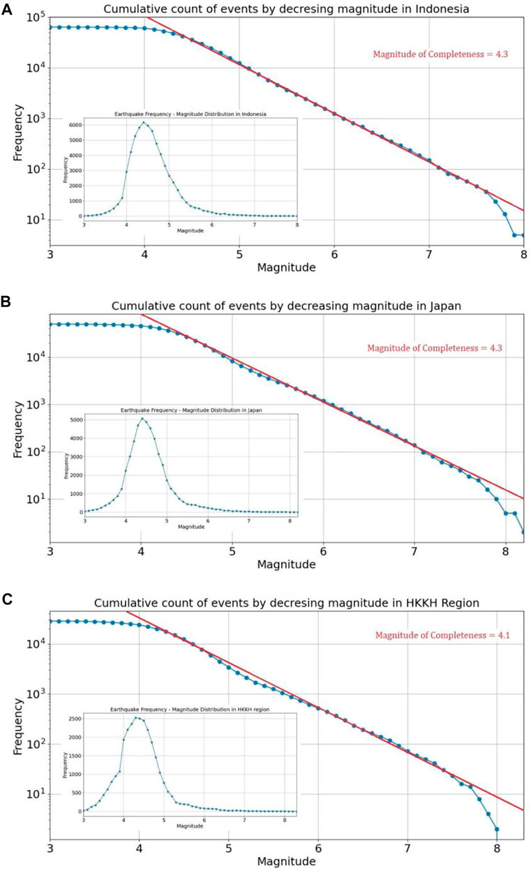
FIGURE 6. Cumulative count of earthquakes that occurred in (A) Indonesia, (B) Japan and (C) HKKH Region ordered by decreasing magnitude on a logarithmic scale (main). Frequency—Magnitude distribution in seismic catalogs of (A) Indonesia, (B) Japan and (C) HKKH Region (inset).

In this study, global temperature anomaly data, along with eight seismic parameters, were utilized to determine the seismic potential of any region. The parameters are selected based on Gutenberg Richter’s law of earthquake magnitude distributions, and recent earthquake prediction research (Panakkat and Adeli, 2007; Panakkat and Adeli, 2009; Asim et al., 2018). The number of instances in each of the three datasets varies according to the seismic events recorded in the catalogues of the individual regions. Before processing seismic parameter computation, the earthquake database is purged of all seismic events with magnitudes below the threshold. This eliminates erroneous or incomplete data in determining seismic parameter trends. The most recent 100 records prior to each earthquake event have been considered to calculate these seismic parameters. These parameters are then used along with global temperature anomaly data to forecast the magnitude of the next earthquake.

A vector of seismicity characteristics created for each preceding significant seismic event as well as the monthly global temperature anomaly are the inputs for the deep neural network. Each seismic zone is unique, and different seismic parameters display various characteristics. Consequently, independent training of the LSTM, Bi-LSTM, and transformer models is conducted using 80% of the available seismic records in the relevant datasets for each area. After the models have been trained, the results are evaluated against the remaining 20% of the datasets. Figure 7 depicts the overall flowchart of the suggested research technique for estimating the magnitude of an impending earthquake.

FIGURE 7

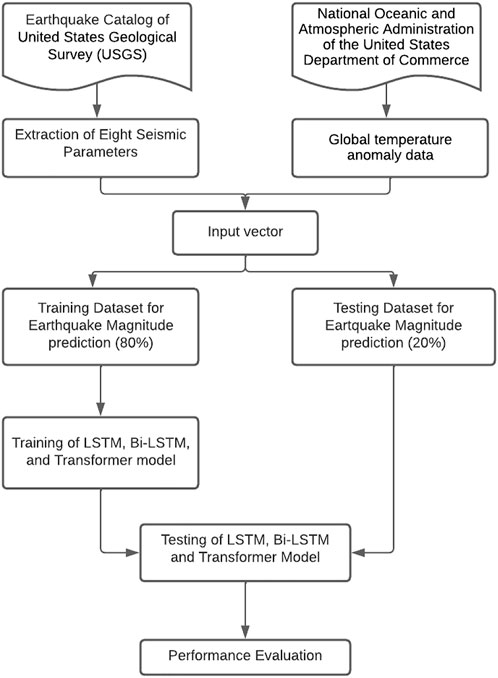
FIGURE 7. Research methodology used in this research.

3.1 Seismic parameters

The investigation of seismic parameters and their computations are inspired by the work (Panakkat and Adeli, 2007; Adeli and Panakkat, 2009; Panakkat and Adeli, 2009). Eight parameters were derived from seismic catalogs to predict the magnitude of an imminent earthquake. The most recent $n$ records ($n$ = 100) prior to each earthquake event are used to calculate these earthquake parameters. These parameters are then used along with global temperature anomaly data to forecast the magnitude of the next earthquake. The parameters are numerical representations of seismic facts such as the Gutenberg–Richter law, foreshock frequency, seismic energy release, and typical temporal earthquake magnitude distribution. Consequently, a feature vector of eight parameters depicts the region’s internal geological state prior to each earthquake occurrence.

3.1.1 Time elapsed ($T$) for the last “$n$” seismic events

The first seismic parameter addressed in this study is time $T$, which reflects the time interval between the last $n$ occurrences, where $n$ is 100 in our study and $t$ is the time of the earthquake.

$T=t_n-t_1$

Most earthquakes are preceded by significant precursor activity, such as a series of foreshocks. Indeed, some of the most popular earthquake prediction models (Zaliapin et al., 2003) are based on the frequency and intensity of foreshocks. The foreshock frequency can be measured using the $T$ value, which depends on the set magnitude threshold. A high $T$ value indicates a dearth of foreshocks, which may indicate a diminished likelihood of a subsequent large seismic event in many seismic zones. On the other hand, a small $T$ value indicates a relatively high foreshock frequency and an increased probability of a subsequent large seismic event.

3.1.2 The mean magnitude ($M_{mean}$)

The second seismic parameter is the average magnitude of the 100 most recent earthquakes. It is proportional to the magnitudes of foreshocks since the seismic activity of magnitude $M$ increases just before a large earthquake.

$M_{mean}=\frac{\sum M_i}{n}(2)$

Following the accelerated release theory (Bufe and Varnes, 1993), the quantity of energy released by a fractured fault increases exponentially as the period between earthquakes decreases. In other words, the measured mean magnitudes of foreshocks increase just prior to the occurrence of a large earthquake.

3.1.3 The slope of the Gutenberg-Richter curve ($b$—value)

The Gutenberg–Richter inverse power law is utilized to illustrate the relationship between the number of earthquakes $n$ with a magnitude equal to or higher than $M$,

$\log \left(n\right)=a-bM(3)$

where parameter $a$ denotes the intensity of seismicity and parameter $b$ represents the ratio of minor to major events. These are the two seismic parameters considered in this study. The $b$-value determines the frequency of smaller earthquakes relative to larger ones: the greater the $b$-value, the more frequent smaller earthquakes. Multiple studies link the b-value to the Earth’s crust’s differential stress, with low b-values seen in highly strained zones or faults and high b-values in less stressed locations. Using the maximum likelihood (ML) method, the b-value can be calculated as follows:

$\widehat{b}=\frac{1}{\ln \left(10\right)\left(M_{mean}-M_c\right)}(4)$

where $M_c$ and $M_{mean}$ are the magnitudes of completeness of the catalogue and the mean magnitude of past $n$ events ($n$ is 100), respectively.

3.1.4 The y-intercept of the Gutenberg-Richter curve ($a$ value)

The values of $a$ and $b$ in the Gutenberg–Richter inverse power law provide a regression line that can estimate future earthquake frequencies. The G-R distribution has constant parameters $a$ and $b$. The expression below represents the value of $a$

$\widehat{a}={\mathit{log}}_{10}\left(\frac{N\left(M\right)}{T}\right)+b{M}_c;M\ge M_c(5)$

where $N\left(M\right)$ represents the number of earthquakes of a specific magnitude $M$.

3.1.5 Magnitude deficit ($∆M$)

The magnitude deficit is another seismic parameter in this study. Based on the Gutenberg and Richter (1956) relationship, it measures the difference between the largest observed magnitude and the largest predicted magnitude.

$∆M=M_{\mathit{max},observed}-M_{\mathit{max},expected}(6)$

where $M_{\mathit{max},observed}$ is the maximum magnitude observed in the previous $n$ events and $M_{\mathit{max},expected}$ is the largest magnitude projected by the inverse power-law relationship in the previous $n$ occurrences. Due to the probability that an event of the largest magnitude would occur only once among $n$ occurrences, $N$ = 1, log $N$ = 0, and Eq. 3 yields

$M_{\mathit{max},expected}=\frac{a}{b}(7)$

3.1.6 Rate of the square root of the seismic energy ($d{E}^{1/2}$)

The rate of the square root of seismic energy release $\left(dE\right)$ is another seismic parameter associated with seismic activity. Most seismic zones are open physical systems with a constant accumulation of energy induced by lithospheric plate movement. These systems retain relative equilibrium if frequent low-magnitude seismic activity dissipates the increasing accumulation of energy (Roeloffs, 2000). When low-magnitude seismic activity is halted for an extended period due to frictional or mechanical causes, the physical system conserves energy; this phenomenon is known as “seismic quiescence.” When the accumulated energy exceeds a predetermined level, it is released as a large seismic event (Tiampo, Rundle, McGinnis, Gross, and Klein, 2002). Hence, the rate at which seismic energy is emitted is a critical parameter of seismicity in quiescent environments. The following equation represents the square root of the seismic energy released.

$d{E}^{1/2}=\frac{\sum E^{1/2}}{T}(8)$

where $E^{1/2}$ is the square root of seismic energy ($E$), determined from the associated Richter magnitude and expressed in ergs by the following empirical relation.

$\left(E\right)={10}^{\left(11.8+1.5M\right)}(9)$

3.1.7 Sum of mean square deviations from the regression line using the Gutenberg-Richter inverse power law ($\eta$—value)

This metric assesses the degree to which observed seismic data conform to the Gutenberg-Richter inverse power-law relationship. Lower values indicate that it is more likely that the observed distribution may be approximated by the power law. In contrast, larger values indicate increased unpredictability and the inability of the power law to represent magnitude-frequency distributions.

$\eta =\frac{{\displaystyle \sum }{\left({\mathit{log}}_{10}{N}_i-\left(a-b{M}_i\right)\right)}^2}{\left(n-1\right)}(10)$

3.1.8 Mean time between characteristic events ($\mathrm{\mu }$)

This is the average duration or interval between occurrences of a particular attribute over the past $n$ instances. According to the elastic rebound hypothesis (Reid, 1910), certain seismic zones demonstrate periodic trends in the slow accumulation of stress and eventual release via large earthquakes. Researchers have shown that the time between large earthquakes is rather consistent (Kagan and Jackson, 1991). Large earthquakes of this magnitude are known as typical occurrences. In this context, magnitudes are provided within a certain approximation range. For example, earthquakes of magnitudes between 5 and 5.5 are considered to have the same typical magnitude. Ideally, typical occurrences occur at roughly equal intervals of time. Suppose $t_{iCharecteristic}$ denotes the observed time interval between characteristic occurrences of magnitude $M_i$, and the total number of characteristic events is represented by $n_{Charecteristic}$. In that case, the mean time between characteristic occurrences ($\mathrm{\mu }$) can be calculated using the following equation:

$\mathrm{\mu }=\frac{\sum \left(t_{iCharecteristic}\right)}{n_{Charecteristic}}(11)$

The input of the deep neural network is a vector of seismicity parameters generated for each prior significant seismic event and the global temperature anomaly for the month. A collection of seismic parameters exhibiting maximum performance in one region may not do so in other region. Additionally, global temperature anomalies have a substantial impact on earthquakes. Together with the global temperature anomaly, all seismic parameters are employed concurrently to construct a deep learning-based model for earthquake magnitude prediction. The next section provides an overview of the deep neural network models utilized in this study.

4 Analytical methods

This section gives a concise summary of the analytical procedures utilized in this investigation.

4.1 Deep neural networks

Neural network architecture is generally used to implement deep learning. Deep neural networks use a series of non-linear processing layers, with basic components operating in parallel. It consists of an input layer, several concealed layers, and an output layer. Nodes or neurons connect the various levels. Each hidden layer uses the output of the preceding layer as its input. In data science, deep learning has emerged as a powerful technique for tackling previously intractable problems in the natural world (Sadowski and Baldi, 2018; Bourilkov, 2019). This is assisted by deep learning’s enhanced capacity to find intricate patterns in extremely large datasets.

Long-term contextual information is mostly accessible in the internal states of the network, where these activities are stored. Recurrent neural networks (RNNs) are a robust modelling method for such sequential data because of their cyclic connections. RNNs are highly effective in applications involving the labelling and prediction of sequences. Recurrent neural networks use inputs from previously active networks to improve predictions. This method allows RNNs to employ a dynamic contextual window over the input sequence instead of the static contextual window used by feed-forward networks (Sak et al., 2014).

4.1.1 Long short-term memory recurrent neural network

LSTM networks are a special kind of recurrent neural network that are designed to recognize the importance of context in making sequence predictions. LSTM networks were first proposed in 1997 by Hochreiter and Schmidhuber (1997). LSTM is a kind of RNN that overcomes the difficulties of handling long-term dependencies (Graves, 2014). In addition, LSTMs do not suffer from the vanishing gradient problem (Hochreiter, 1998; Gers et al., 2000). LSTMs have feedback connections, in contrast to deep feed-forward neural networks. In both context-free and context-sensitive language learning, LSTM models outperform RNNs (Gers and Schmidhuber, 2001). In addition to handling single data points in vectors or arrays, they can handle data sequences. Because of this, LSTMs excel in processing and predicting time series.

The LSTM model, in contrast to the RNN’s hidden layer neurons, is made up of a unique collection of memory cells. The LSTM model is dependent on the state of the entity. The gate structure filters information to maintain and refresh the state of memory cells. The gate structure includes input, forget, and output gates. There are three sigmoid layers and one tanh layer in every memory cell (Qiu et al., 2020). The forget gate $f_t$ of the LSTM unit determines which cell state information is omitted from the model. The memory cell translates the previous moment’s output $h_{t-1}$ and the current moment’s external information $x_t$ into a long vector [$h_{t-1}$, $x_t$] to represent the current moment.

$f_t=\sigma \left(W_f.\left[h_{t-1},x_t\right]+b_f\right)(12)$

$W_f$ and $b_f$ are the forget gate’s weight matrix and bias, respectively, and σ is the sigmoid function. The forget gate’s primary function is to monitor how much of the prior cell state $C_{t-1}$ is reserved for the current cell state $C_t$. The gate outputs a value between 0 and 1 based on $h_{t-1}$ and $x_t$, with 1 signifying total reserve and 0 indicating total discard. The input gate $i_t$ regulates the amount of the current time network input $x_t$ reserved for the cell state $C_t$, avoiding unnecessary data from entering memory cells. The first step is determining which cell state has to be modified; the sigmoid layer chooses the modified value, as illustrated in Eq. 13. The alternative option is to modify the cell state’s data. Using the tanh layer, a new candidate vector $\widehat{C_t}$ is generated to govern the amount of new information provided, as indicated by Eq. 14.

$i_t=\sigma \left(W_t.\left[h_{t-1},x_t\right]+b_i\right)(13)$

$\widehat{C_t}=\tanh \left(W_c.\left[h_{t-1},x_t\right]+b_c\right)(14)$

The final step is to update the cell states of the memory cells using Eq. 15

$C_t=f_t*C_{t-1}+i_t*\widehat{C_t}(15)$

The $O_t$ output gate controls how much of the current cell state is discarded.

$O_t=\sigma \left(W_{\sigma }.\left[h_{t-1},x_t\right]+b_o\right)(16)$

The final output value of the cell is stated as

$h_t=O_t*\tanh \left(C_t\right)(17)$

4.1.2 Bidirectional long short-term memory recurrent neural network

Bidirectional networks provide significant advantages over unidirectional networks in a variety of contexts (Cui et al., 2022). Bidirectional LSTM is derived from bidirectional RNN (Schuster and Paliwal, 1997), which employs two hidden layers to examine sequence input in both forward and backward directions. Two hidden layers are connected to the same output layer through bidirectional LSTMs. Using positive sequence inputs from time $T-n$ to time $T-1$, the forward layer generates a sequence of output values, denoted by $\overrightarrow{\mathit{h}}$. In contrast, the reverse layer generates a sequence of values, denoted by $\stackrel{⃖}{\mathit{h}}$, using inverted sequence inputs from time $T-n$ to time $T-1$. The outputs of the forward and backwards layers are calculated using the conventional LSTM Eqs 12–17. The bidirectional LSTM layer generates the ${\mathit{Y}}_T$ output vector, whose elements are determined using the equation.

$y_t=\sigma \left(\overrightarrow{h},\stackrel{⃖}{h}\right)(18)$

Here, the $\sigma$ function is used to mix the two output sequences. It may be a function of summation, average, concatenation, or multiplication. Using earthquake magnitude prediction as an illustration, the final output of a bidirectional LSTM layer may be expressed in the form of a vector, $Y_T\left[y_{T-n},\dots y_{T-1}\right]$, where the last element, $y_{T-1}$, indicates the expected magnitude of the next earthquake.

4.1.3 Transformer model

The self-attention-based transformer for sequence modelling has recently been introduced and has been a tremendous success (Parikh et al., 2016; Vaswani et al., 2017). In contrast to RNN-based approaches, the transformer model may access any historical segment regardless of distance. It excels at recognizing recurring patterns with long-term dependencies. The performance benefits of transformer models in prediction have been widely established (Li et al., 2020). Numerous recent studies have applied it in image, music, and speech processing (Huang et al., 2018; Parmar et al., 2018; Povey et al., 2018). However, scaling attention to extremely long sequences is computationally expensive since the space complexity of self-attention rises quadratically with sequence length (Huang et al., 2018). When forecasting time series with exact precision and substantial long-term dependence, this becomes a serious issue. In addition, the space complexity of the canonical transformer, which rises quadratically with input length $L$, may create a memory bottleneck. The sparse transformer (Child et al., 2019), with a complexity of $O(n\sqrt{n}$), and the sparse log transformer (Li et al., 2020), with a complexity of $O\left({n\left(\log n\right)}^2\right)$, are some solutions to this problem. These methods have made it possible to simulate long-term time series.

The transformer model is composed of encoders and decoders. Each encoder layer’s primary responsibility is to create data describing relationships between inputs. In contrast, the decoder component takes all the encoded data and uses the embedded context information to produce a new sequence of output values. Both the encoder and decoder are built of modules that may be layered on top of one another. The bulk of modules are composed of multi-head attention and feed-forward layers. The attention mechanism translates a query and a collection of key-value pairs to output in this instance. The encoder consists of six identical layers with two sublayers stacked together. The first is a multi-head self-attention layer, while the second is a simple position-wise, fully connected feed-forward network. In addition, a residual connection is created surrounding each sublayer, followed by a normalizing layer. Similar to the encoder, the decoder consists of six layers with the same sublayers. Furthermore, multi-head attention is applied to encoder outputs to help in the production of target translations.

The attention function in a transformer is a mapping of a query and an arrangement of key-value sets to output, with the query, keys, values, and output all being vectors. The input consists of queries and keys in dimension $d_k$ and values in dimension $d_v$. Each query is multiplied by all keys and then divided by $\sqrt{d_k}$. The result is a weighted sum of the values, with each value receiving a weight defined by the compatibility function of the query with its corresponding key. The softmax function is then used to obtain weights for the values from the output. In practice, we calculate the attention function in parallel on a set of queries, keys, and values and store the results in a matrix $Q$, $K$, and $V$. The calculation for the output matrix is as follows:

$Attention\left(Q,K,V\right)=softmax\left(\frac{Q{K}^T}{\sqrt{d_k}}\right)V(19)$

4.2 Evaluation criteria

To evaluate the performance of these deep learning models, the following four evaluation criteria were considered: mean absolute error (Willmott and Matsuura, 2005), mean square error (Pishro-Nik, 2014), log-cosh loss (Grover, 2021) and mean squared logarithmic error (Mean Squared Logarithmic Error Loss, 2021).

4.2.1 Mean absolute error (MAE)

The MAE refers to the average absolute vertical or horizontal distance between each point in a scatter plot and the straight line through the origin. Consequently, MAE indicates the average absolute difference between projections and objectives. Thus, MAE assesses how well a forecast matches the actual results.

$MAE=\frac{1}{n}{\displaystyle \sum }_{i=1}^n〈y_i-{\widehat{y}}_i〉(20)$

4.2.2 Mean square error (MSE)

The MSE reflects the deviation between the forecasts and the original projections. It is the average squared deviation between the prediction and the target. Since it is dependent on a square term, negative values are impossible. Thus, it comprises both the estimator’s variance and its bias. The MSE is the sample standard deviation of the differences between anticipated and observed values for the specified number of observations.

$MSE={\left(\frac{1}{n}{\displaystyle \sum }_{i=1}^n{〈y_i-{\widehat{y}}_i〉}^2\right)}^{\frac{1}{2}}(21)$

4.2.3 Log-cosh loss

In regression problems, the $Logcosh$ loss is another smoother metric than the MSE. $Logcosh$ computes the logarithm of the hyperbolic cosine of the prediction error (Grover, 2021).

$\left.Logcosh\left(t\right)={\displaystyle \sum }_{p\in P}\mathit{log}(\mathit{cosh}\left(p-t\right)\right)(22)$

where $p$ denotes the predicted value and $t$ represents the true value. $\mathit{Log}\left(\mathit{cosh}\left(x\right)\right)$ is generally equivalent to $\left(x**2\right)/2$ for small $x$ and $abs\left(x\right)-\mathit{log}\left(2\right)$ for large $x$. This shows that $Logcosh$ behaves similarly to the mean squared error but is less affected by the occasional drastically incorrect predictions (Chris, 2019).

4.2.4 Mean squared logarithmic error (MSLE)

The mean squared logarithmic error is the average of the squared differences between the log-transformed actual and forecasted values over the observed data.

In general, the above formula expresses the loss function:

$L\left(y,\widehat{y}\right)=\frac{1}{N}{\displaystyle \sum }_{i=0}^N{\left(\log \left(y_i+1\right)-\log \left({\widehat{y}}_i+1\right)\right)}^2(23)$

where $\widehat{y}$ denotes the predicted value. This loss may be understood as a ratio between the actual and anticipated values over time.

$\log \left(y_i+1\right)-\log \left({\widehat{y}}_i+1\right)=\log \left(\frac{y_i+1}{{\widehat{y}}_i+1}\right)(24)$

The addition of “1”to both $y$ and $\widehat{y}$ is for mathematical convenience, as $\log \left(0\right)$ is not defined, and both $y$ and $\widehat{y}$ can be zero.

5 Model architecture and training

This work uses deep learning methods to provide predictions regarding the magnitude of future earthquakes based on temperature anomalies and eight other seismic parameters for a specific location. The vectors consisting of temperature anomaly data and eight seismic parameters are fed into neural networks with two types of recurrent units: long short-term memory cells and bidirectional long short-term memory cells. These vectors are also supplied into a transformer model that employs an attention mechanism by variably weighting the significance of each incoming data element. Because each region has unique features and is distinct from others, independent training was conducted to construct a prediction model based on seismic parameters that are distinctive to each region.

5.1 LSTM model

There are 32 LSTM units in the primary layer of the LSTM model. To prevent overfitting, a dropout layer is applied thereafter at a rate of 0.2. When a system is overfitted, it might produce good training results but poor testing outcomes. Overfitting occurs when a system depends excessively on its historical data, rendering it rigid and incapable of adjusting to new input. After that, we have two layers of dense units connected by a linear layer, another layer of dense units activated by a rectified linear unit (ReLU), and a third dense unit serving as the output. The output layer itself consists of a single dense unit.

The number of epochs and batch size are two trivial hyperparameters that must be determined prior to training based on experience and extensive trial and error. The number of epochs is a hyperparameter that controls how many times the learning algorithm will iterate through the training dataset. One epoch denotes that every sample in the training dataset has had the opportunity to influence the internal model parameters. The batch size is a hyperparameter that determines how many samples should be processed before modifying the internal model parameters. Here, we pick batch sizes of 128 and 50 epochs using a regional earthquake catalogue, including thousands of earthquake events (data rows). This means that the dataset is divided into subsets consisting of 128 samples each. After every 128 samples, the model weights are recalculated. The model examines the entire dataset fifty times using fifty epochs.

The model’s architectural representation is shown in Figure 8A. Figure 9 shows the learning graph generated by deep learning models (LSTM, Bi-LSTM, and transformer) utilizing the processed dataset of three seismic zones. A learning curve is a graph that illustrates how the learning performance of a model varies with experience or time. Learning curves are frequently utilized in deep neural network algorithms that learn gradually and adjust their internal parameters over time. The major goal of our work with deep neural networks is to reduce error as much as possible. The objective function is typically characterized by a loss function, with “loss” referring simply to the value produced by the loss function. In this study, all three sets of seismic catalogs were used to build learning curves during the training phase, and the default loss function used was mean square error loss. Low scores suggest higher learning, while a zero score shows that the training dataset was learned accurately and without any mistakes. Here, the training loss plot reduces to the point of stability with a minimal number of epochs, indicating a satisfactory fit of the model with three seismic catalogs.

FIGURE 8

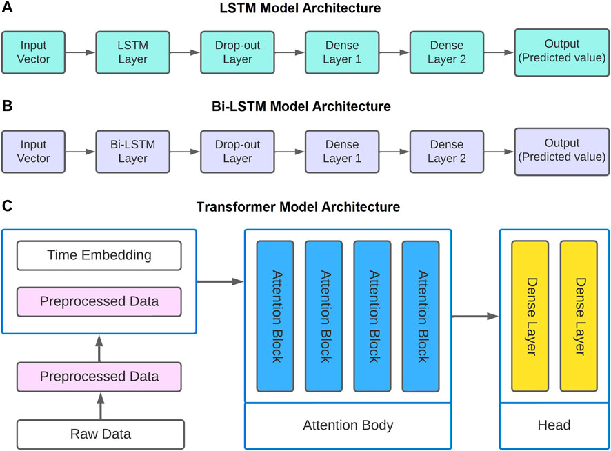
FIGURE 8. Architecture of (A) LSTM, (B) Bi-LSTM and (C) Transformer Model used in this research.

FIGURE 9

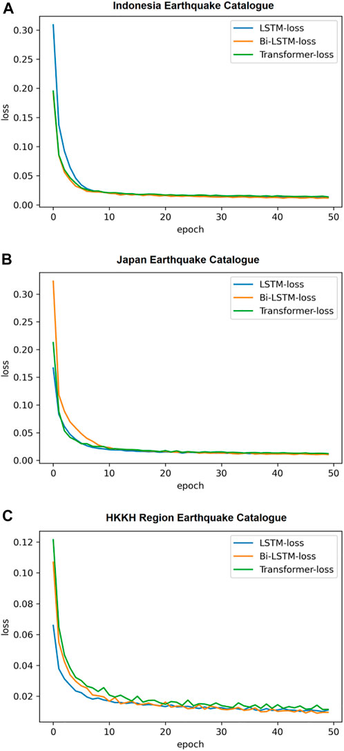
FIGURE 9. Learning graph of the LSTM, Bi-LSTM and transformer models using (A) Indonesia Earthquake Catalogue, (B) Japan Earthquake Catalogue and (C) HKKH Region Earthquake Catalogue.

5.2 Bi-LSTM model

In the Bi-LSTM model, the main layer comprises twenty-four LSTM units that can operate in both directions. To prevent overfitting, the subsequent layer is a dropout layer with a dropout rate of 0.2. The next layers are also unchanged: a layer of dense units activated by a ReLU function, another layer of dense units connected linearly, and a final dense unit serving as the output. The final output layer consists of a single dense output unit. Figure 8B displays an architectural depiction of the model. Figure 9 displays the training loss plot’s gradual decline to stability after a few epochs, indicating that the model fits the three seismic datasets well.

5.3 Transformer model

Here, a multi-head self-attention system has been implemented. This method employs self-attention processes to model sequence data to identify complex correlations of varied lengths from time-series data. Furthermore, this transformer-based technique may describe a wide spectrum of non-linear dynamical systems. The Q, K, and V configurations depend on the input via various thick layers. The next section is optional and depends on the scale of our model and data. However, we will also completely bypass the decoder. This indicates that just one or more layers of the attention block will be utilized. In the last phase, a few thick layers will be employed to estimate anything we want to predict. Figure 8C depicts the model’s implemented architecture.

Each attention block comprises a feed-forward block, a self-attention block, and a normalization block. The sizes of the inputs and outputs for each block are the same. Adam (Kingma and Ba, 2015) is an excellent initial optimizer for training that has been used in this research. Dropout approaches for regularization are applied in the encoder’s and decoder’s three types of sublayers: self-attention, feed-forward, and normalization. The dropout rate for each sublayer is 0.2. The training loss plot stabilizes after a few epochs, as shown in Figure 9, demonstrating a decent model fit to the three seismic datasets.

6 Results and observations

This study attempts to estimate the magnitude of incoming earthquakes based on fluctuations in global temperature and eight seismic parameters of the previous 100 earthquake events by utilizing prominent deep learning algorithms, including LSTM, Bi-LSTM, and transformer. Three datasets from different places, namely, Indonesia, Japan and the HKKH areas, are utilized to test the proposed system’s performance. The training stage employed 80% of the total dataset for each area, with the remaining 20% used in the testing stage. A network makes every attempt to forecast outcomes as precisely as possible. The cost function determines the network’s accuracy by penalizing it when it fails. The best result is the one with the lowest cost. During training, a repetition phase is commonly conducted by separating the training data into equal-sized batches. The number of samples per batch is a hyperparameter that is normally established via trial and error. An epoch is the number of iteration steps in a neural network. The network simulates the time series data once in each epoch. The number of epochs is the most important parameter in the prediction task. With fewer epochs, the model’s accuracy is poor, and the error is greater. By increasing the number of iterations, the model finally converges to the point where the results of two subsequent epochs do not differ considerably. Because of computational resource constraints, the value of this parameter in the LSTM, Bi-LSTM, and transformer is set to 50.

Another aspect influencing model accuracy is the number of neurons in the hidden layers. If it is set too high, overfitting might occur, and the model will be incapable of effectively imitating the data. Dropout layers have been utilized to address this difficulty, which deactivates numerous neurons. Four metrics have been employed to assess the performance of these models: mean absolute error (MAE), mean squared error (MSE), log-cosh loss, and mean squared logarithmic error (MSLE). MAE and MSE are deviation measures that indicate how far the predictions are from the target values. Prediction models perform better when these deviation values are smaller. The log-cosh loss is the logarithm of the prediction error’s hyperbolic cosine. MSLE is the time-dependent ratio between true and anticipated values. The MAE, MSE, log-cosh loss, and MSLE values all started to converge after running these deep learning models on the training dataset.

6.1 Results for Indonesia earthquake catalogs

By examining pre-processed seismic datasets from Indonesia, deep learning algorithms were utilized to investigate the influence of global temperature fluctuations on earthquake occurrences and evaluate how the actual and predicted magnitudes vary over time. Figure 10 illustrates this. Based on our observations, these models can project magnitudes ranging from 3.8 M to 5.8 M. Figure 11 depicts the predicted magnitude as a function of the observed magnitude. The x-axis represents the model’s projected magnitude, while the y-axis represents the observed or actual magnitude recorded in the seismic dataset. The diagonal line in the plot’s centre represents the estimated regression line. Because each data point is quite close to the anticipated regression line, we can conclude that the LSTM model fits the data fairly well. The figure also indicates that the model can predict earthquakes up to 5.8 M. Figure 12 shows a histogram of the errors produced by a deep neural network when forecasting the magnitude of the next upcoming earthquake. The difference between actual and projected values is referred to as “errors.” These error numbers may be negative since they represent the extent to which the projected values differ from the actual values. The bulk of the anticipated magnitudes have errors near 0.0, with larger deviations being rare. The distribution is approximately symmetrical, with LSTM model values ranging from −0.2 to 0.2. As shown in Figure 13, the performance of each deep learning model improved as the deviation metrics decreased with increasing epochs. Tables 2 compare all deviation metrics calculated by the models used in the Indonesia earthquake datasets during training and testing. On the Indonesia earthquake dataset, all models performed well. As demonstrated in Table 2, the Bi-LSTM model had the lowest deviation metrics throughout the training period. When these models were fed an unknown test dataset, the LSTM model outperformed the others with the lowest deviation metrics. In the testing stage, the LSTM model surpasses the others, with the lowest MAE = 0.066, MSE = 0.007, log cosh loss = 0.039, and MSLE = 0.003.

FIGURE 10

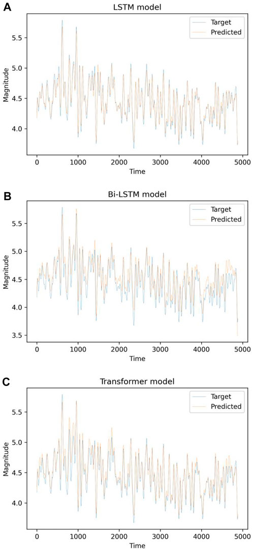
FIGURE 10. Plot of projected and actual magnitude as a function of time for the Indonesia earthquake catalogue using the (A) LSTM, (B) Bi-LSTM, and (C) transformer models.

FIGURE 11

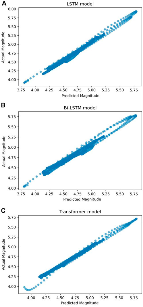
FIGURE 11. Plot of observed magnitude against anticipated magnitude utilizing (A) LSTM, (B) Bi-LSTM, and (C) transformer models on the Indonesia earthquake catalogue.

FIGURE 12

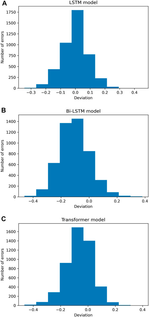
FIGURE 12. Error distribution of the (A) LSTM, (B) Bi-LSTM, and (C) transformer models applied to the Indonesia earthquake catalogue.

FIGURE 13

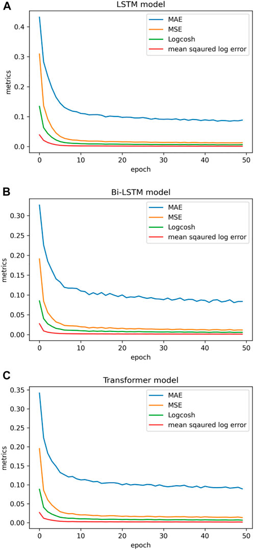
FIGURE 13. Performance metrics using (A) LSTM, (B) Bi-LSTM, and (C) transformer model on the Indonesia earthquake catalogue.

TABLE 2

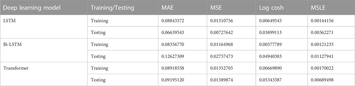
TABLE 2. Results of different models during training and testing using Indonesia Dataset.

6.2 Results for Japan earthquake catalogs

Deep learning methods were utilized to evaluate the pre-processed seismic data from Japan. The study evaluates how the predicted and actual magnitudes vary over time, as shown in Figure 14. These models can predict magnitudes ranging from 3.8 M to 5.8 M based on our observations. Figure 15 illustrates the predicted magnitude as a function of the observed magnitude. The x-axis indicates the model’s predicted magnitude, while the y-axis represents the observed or true magnitude recorded in the seismic database. Because each data point is relatively near the predicted regression line, we can infer that the transformer model, fits the data fairly well. The figure also indicates that the model can predict earthquakes with magnitudes up to 5.8 M.

FIGURE 14

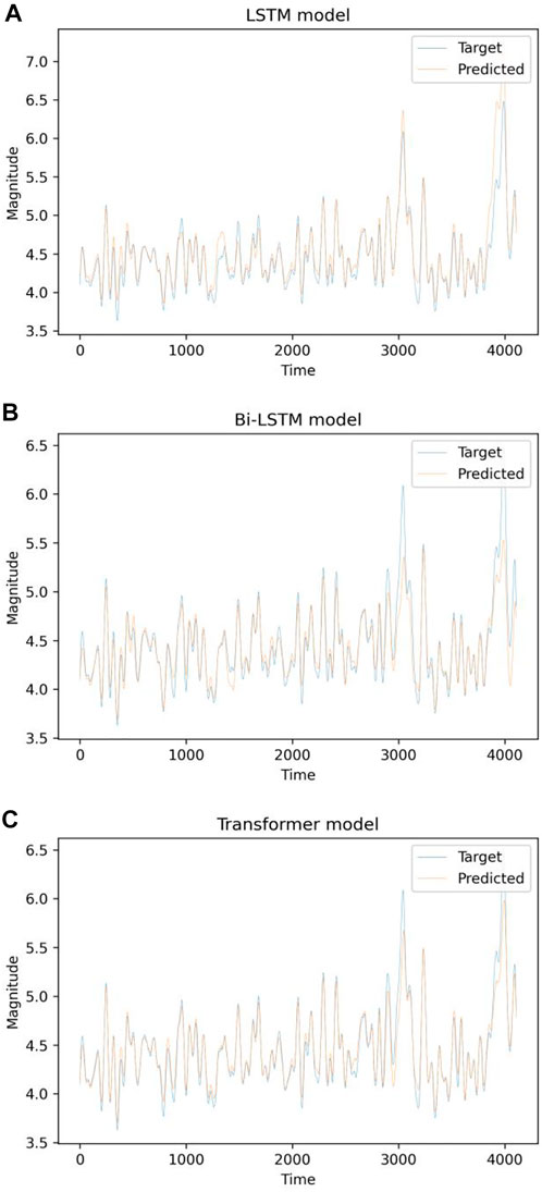
FIGURE 14. Plot of projected and actual magnitude as a function of time for the Japan earthquake catalogue using the (A) LSTM, (B) Bi-LSTM, and (C) transformer models.

FIGURE 15

FIGURE 15. Plot of observed magnitude against anticipated magnitude utilizing (A) LSTM, (B) Bi-LSTM, and (C) transformer models on the Japan earthquake catalog.

Figure 16 shows the distribution of errors made by a deep neural network when predicting the magnitude of the next impending earthquake. Most anticipated magnitudes have errors near 0.0, whereas greater discrepancies are uncommon. The distribution of errors for the LSTM and transformer model is confined within the range from −0.2 to 0.2, indicating a roughly symmetrical distribution. Figure 17 depicts how each deep learning model’s performance was enhanced as the deviation metrics dropped with increasing epochs. Table 3 compare all the deviation metrics produced by these models in the Japan earthquake datasets during training and testing. The Bi-LSTM model obtained the lowest deviation metrics during the training period, as shown in Table 3. The transformer model outperformed the other models with the fewest deviation metrics when fed with an unknown test dataset. In the testing phase, the transformer model surpasses the others, with the lowest MAE = 0.083, MSE = 0.015, log cosh loss = 0.054, and MSLE = 0.007.

FIGURE 16

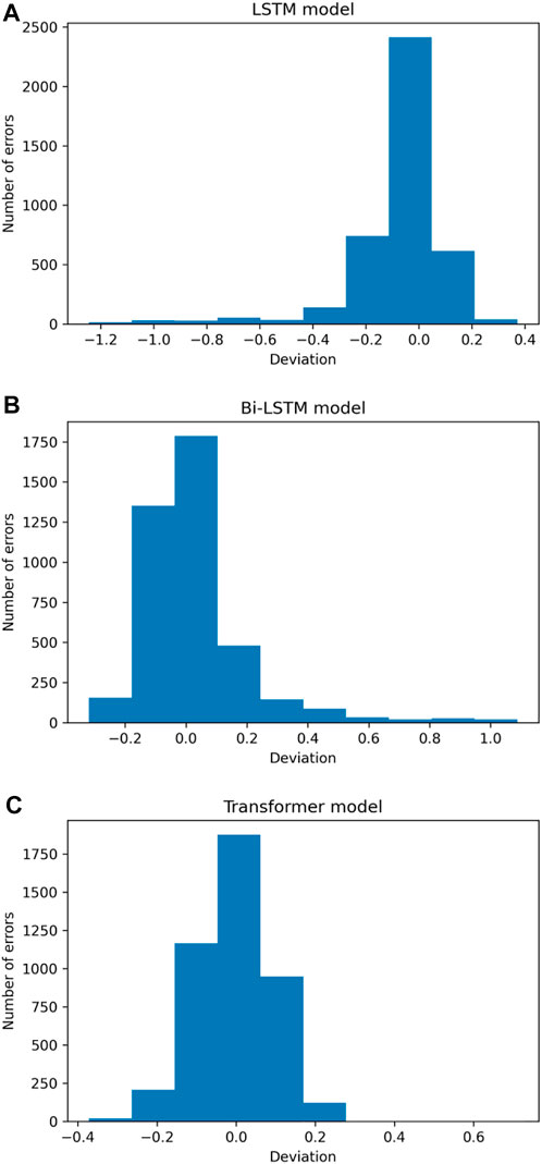
FIGURE 16. Error distribution of the (A) LSTM, (B) Bi-LSTM, and (C) transformer models applied to the Japan earthquake catalogue.

FIGURE 17

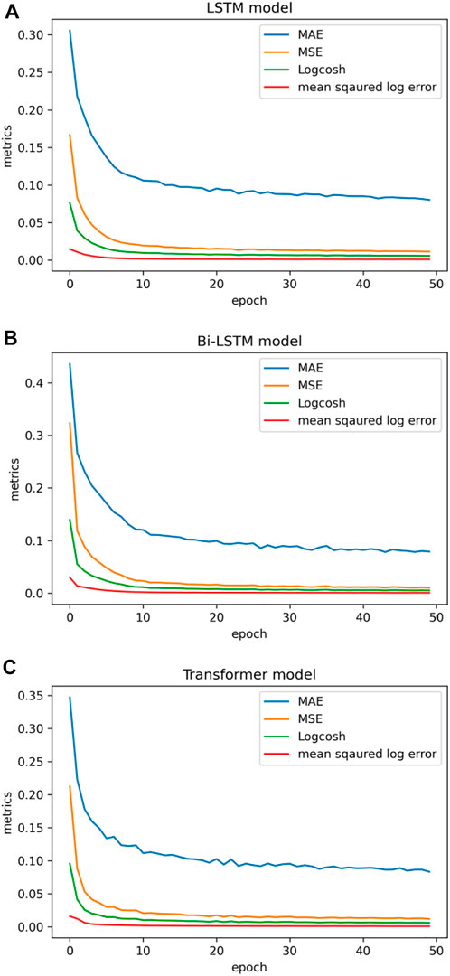
FIGURE 17. Performance metrics using (A) LSTM, (B) Bi-LSTM, and (C) transformer model on the Japan earthquake catalogue.

TABLE 3

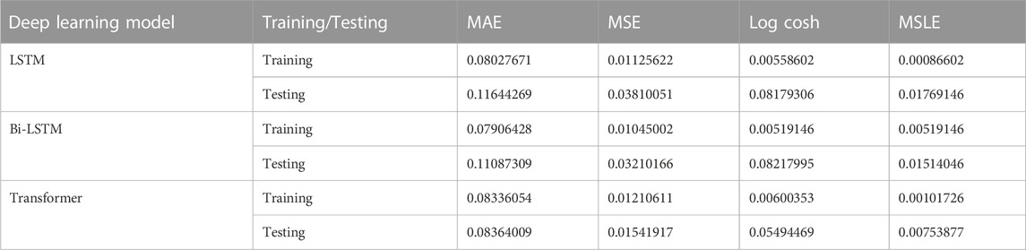
TABLE 3. Results of different models during training and testing using Japan Dataset.

6.3 Results for HKKH region earthquake catalogs

Deep learning techniques were also used to examine pre-processed seismic data from the HKKH area. Figure 18 illustrates the temporal evolution of the projected and actual magnitudes. According to our findings, these models can estimate magnitudes ranging from 3.5 M to 5.2 M. Figure 19 depicts the expected magnitude as a function of the observed magnitude. The x-axis represents the model’s projected magnitude, while the y-axis represents the observed or real magnitude recorded in the seismic database. We may infer that the LSTM model fits the data fairly well in contrast to other models because each data point is close to the predicted regression line. Furthermore, the image shows that the model can detect earthquakes with magnitudes of up to 5.3 M. Figure 20 shows a histogram of the errors generated by deep neural networks while estimating the size of an upcoming earthquake. Most of the predicted magnitudes have errors near 0.0, with larger deviations being unusual. In the LSTM model, the distribution is reasonably symmetrical, with values ranging from −0.2 to 0.2. Figure 21 shows how the performance of each deep learning model increased as the deviation metrics dropped with increasing epochs. Table 4 compare all deviation metrics derived from the models in the HKKH area earthquake datasets during training and testing. On the HKKH region earthquake dataset, all models performed brilliantly. As demonstrated in Table 4, the Bi-LSTM model had the lowest deviation metrics throughout the training period. When these models were fed an unknown test dataset, the LSTM model outperformed the others with the lowest deviation metrics. According to Table 4, the LSTM model outperforms the others in the testing phase, with the lowest MAE = 0.083, MSE = 0.011, log cosh loss = 0.039, and MSLE = 0.005.

FIGURE 18

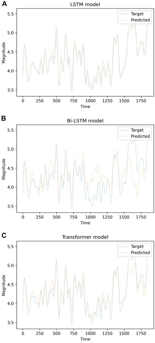
FIGURE 18. Plot of projected and actual magnitude as a function of time for the HKKH region earthquake catalogue using the (A) LSTM, (B) Bi-LSTM, and (C) transformer models.

FIGURE 19

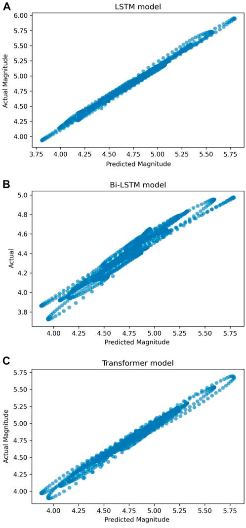
FIGURE 19. Plot of observed magnitude against anticipated magnitude utilizing (A) LSTM, (B) Bi-LSTM, and (C) transformer models on the HKKH region earthquake catalogue.

FIGURE 20

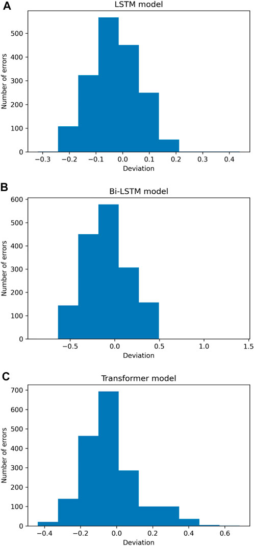
FIGURE 20. Plot of observed magnitude against anticipated magnitude utilizing (A) LSTM, (B) Bi-LSTM, and (C) transformer models on the HKKH region earthquake catalogue.

FIGURE 21

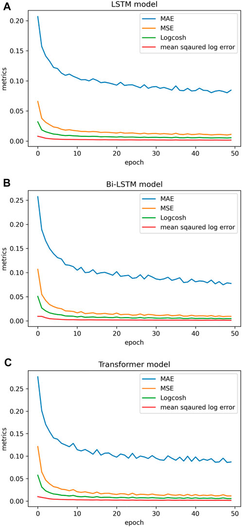
FIGURE 21. Performance metrics using (A) LSTM, (B) Bi-LSTM, and (C) transformer model on the HKKH region earthquake catalogue.

TABLE 4

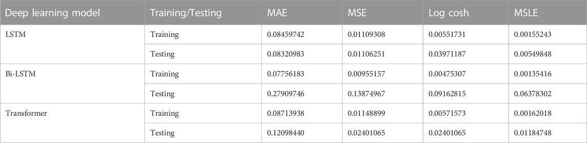
TABLE 4. Results of different models during training and testing using HKKH Region Dataset.

The test results presented in Tables 2–4 demonstrate that these deep learning models can predict the magnitude of an impending earthquake with a maximum MSE of 0.03 across all three regional earthquake catalogs. The errors caused by the models may be approximated to a maximum standard deviation of 0.17 magnitude units over all three datasets. As a result, we can conclude that these models are extremely accurate in modelling these datasets, as the error in the magnitude estimations of mild earthquakes has a maximum standard deviation of 0.17, depending on the network. Consequently, the results indicate that the models make fewer errors in their predictions. As a result, we may deduce that these models accurately simulate the seismic datasets of the three regions and the global temperature data. Alternatively, these models have effectively identified a correlation between earthquake magnitude and global temperature fluctuations.

Using earthquake catalogs from three distinct regions, the performance of the proposed system is assessed in this section. Low MSE, MAE, log cosh, and mean squared log error values indicate that the models fit all three datasets well, indicating a solid prediction system. The models' bias or variance errors are depicted on the training graphs. During the training period, all of the models converged to identical MSE, MAE, log-cosh loss, and MSLE values for all three seismic databases. These evaluation criteria are utilized to evaluate each model’s performance. The convergence of these evaluation metrics to a small number indicates that the models fit the dataset with a high degree of precision, suggesting a correlation between the magnitude of the earthquake and fluctuations in global temperature. All three deep learning algorithms utilized in this study performed well and accurately to predict the magnitude of approaching earthquakes, confirming the efficiency and usefulness of earthquake modelling.

Temperature has a significant impact on growing heat fluxes close to earthquake zones. Sensible heat flow boosts evapotranspiration, one of the processes that moves water vapour into the atmosphere. This may lead to cloud formation and increased precipitation. Strong earthquakes are frequently linked to an increase in precipitation in seismic zones. In addition, climatic change and global warming increase glacier erosion, resulting a shift of mass balance on Earth’s crust. This mass redistribution may enhance the probability of stress release in a previously stressed region. This is because erosion reduces the system’s overall stress, which is sufficient to stabilize the system prior to unloading. Consequently, the loading and emptying of water bodies due to climate change may have direct effects on local seismicity. The impact of climate change on regional and transregional earthquakes, however, needs to be thoroughly investigated.

Most of the hypotheses produced in earthquake precursor signal studies are based on empirical formulas. Multiple factors contribute to the occurrence of an earthquake, including the accumulation of energy caused by tectonic motions, the stress‒strain pattern, the fault types, the dynamics of the inner earth fluid, and the geomorphological structure. Consequently, at the concluding phase of earthquake preparation, extremely complicated precursory signals may be received. On the basis of the precursory signal’s characteristics (amplitude, frequency, and phase), one can provide quantitative information regarding the probable magnitude, depth, location, and timing of next earthquake. However, there has not been much progress made thus far.

7 Conclusion

This study provides a novel method for establishing the association between earthquake occurrences and climate change by employing deep learning and finds a sustainable method for earthquake prediction. This study selected global temperature as the single climatic variable because it substantially impacts the Earth’s ecosystem and civilization. Global temperature data along with several mathematically computed seismic parameters are considered basic inputs for deep learning algorithms. This study presented deep learning-based approaches for forecasting the magnitude of imminent earthquakes utilizing LSTM, Bi-LSTM, and the transformer model with global temperature anomaly data on the earthquake catalogs of Japan, Indonesia, and the Hindu-Kush Karakoram Himalaya area. Approximately 80% of earthquake datasets are utilized to train the deep learning models. The remaining 20% of the data were subsequently predicted. A double hidden layer was employed in the LSTM and Bi-LSTM models, and a multi-head self-attention system was built into the transformer model. The accuracy of a model is very sensitive to various parameters, such as the number of recurrent units in the hidden layers, the batch size, and the number of epochs. Extensive testing was carried out throughout the training phase to identify the optimal values for these parameters. Dropout layers are utilized to prevent overfitting in all models. The effectiveness of these models was assessed using the MAE, MSE, log-cosh loss, and MSLE metrics.

The cost functions for all models with varied earthquake datasets converge to minimal values. For the Indonesia earthquake catalogs, the LSTM model has been found to perform best during testing, with an MAE = 0.066, MSE = 0.007, log cosh loss = 0.038, and MSLE = 0.003. The model also exhibited the lowest MAE = 0.083, MSE = 0.011, log cosh loss = 0.039, and MSLE = 0.005 when tested with an unknown dataset obtained from the seismic catalogue of the Hindu-Kush Karakoram Himalaya region. The transformer model seems to have the lowest MAE = 0.083, MSE = 0.015, log cosh loss = 0.054, and MSLE = 0.007 for the earthquake catalogue of Japan. Achieving such a low value indicates that the models provide a good fit to the data, suggesting a correlation between the magnitude of the earthquake and fluctuations in global temperature. Several regional earthquake catalogs were used to test and validate deep learning-based techniques, and the results showed that the LSTM, Bi-LSTM, and transformer models were the most accurate algorithms for predicting earthquake magnitude. However, the maximum magnitudes anticipated by these models are confined between M5 and M6 depending upon the datasets. Due to the relative scarcity of large seismic occurrences in the historical earthquake records of a few places, particularly within a time span suited for retrospective forecasts, it is difficult to quantify the amount of statistical success in predicting large earthquakes.

The global temperature anomaly is considered as the only climate variable for this investigation since it strongly affects the Earth’s ecosystem and civilization. In this experimental study, melting ice and isostasy have been discussed to explain their relationship with rising global temperatures and their effect on regional seismicity. As per our knowledge concern, no dataset has been publicly available for climatic variables such as precipitation, humidity, air pressure, wind speed, etc. However, considerations of these variables might change in the deep neural network models, and a comparative analysis of earthquake magnitude prediction using temperature and without using temperature both can be an interesting study as a future scope of this work.

A very interesting recent study (Christie et al., 2022) on the eastern Antarctic Peninsula’s Larsen A and B ice shelves points out the need for more in-depth research to establish our claim as more robust and accurate. It is interesting to note that if the study can be carried out based on regional temperature anomalies instead of global temperature anomalies for some specified regions along with seismic data, the findings may be more accurate. From the publicly available dataset, the global temperature anomaly and seismic data of some specified regions are used as inputs in our experimental study. The non-availability of regional temperature anomaly data is indeed a major challenge of this work.

Data availability statement

The original contributions presented in the study are included in the article/supplementary material, further inquiries can be directed to the corresponding author.

Author contributions

All authors contributed to the study conception and design. Material preparation, data collection and analysis were performed by BS. The first draft of the manuscript was written by BS, and all authors commented on previous versions of the manuscript. All authors read and approved the final manuscript.

Conflict of interest

The authors declare that the research was conducted in the absence of any commercial or financial relationships that could be construed as a potential conflict of interest.

Publisher’s note

All claims expressed in this article are solely those of the authors and do not necessarily represent those of their affiliated organizations, or those of the publisher, the editors and the reviewers. Any product that may be evaluated in this article, or claim that may be made by its manufacturer, is not guaranteed or endorsed by the publisher.

References

Abdullah, T., Romshoo, S. A., and Rashid, I. (2020). The satellite observed glacier mass changes over the Upper Indus Basin during 2000–2012. Sci. Rep. 10 (1), 14285. doi:10.1038/s41598-020-71281-7

PubMed Abstract | CrossRef Full Text | Google Scholar

Adeli, H., and Panakkat, A. (2009). A probabilistic neural network for earthquake magnitude prediction. Neural Netw. 22 (7), 1018–1024. doi:10.1016/j.neunet.2009.05.003

PubMed Abstract | CrossRef Full Text | Google Scholar

Ambraseys, N. N., and Melvilleand, C. P. (1983). A history of Persian earthquakes, by N. N. Ambraseys and C. P. Melville, cambridge university press, cambridge, 1982. No. Of pages: 219. Price: £35. Earthq. Eng. Struct. Dyn. 11 (4), 591. doi:10.1002/eqe.4290110412

CrossRef Full Text | Google Scholar

Asim, K. M., Idris, A., Iqbal, T., and Martínez-Álvarez, F. (2018). Seismic indicators based earthquake predictor system using Genetic Programming and AdaBoost classification. Soil Dyn. Earthq. Eng. 111, 1–7. doi:10.1016/j.soildyn.2018.04.020

CrossRef Full Text | Google Scholar

Asim, K. M., Awais, M., Martínez–Álvarez, F., and Iqbal, T. (2017b). Seismic activity prediction using computational intelligence techniques in northern Pakistan. Acta Geophys. 65 (5), 919–930. doi:10.1007/s11600-017-0082-1

CrossRef Full Text | Google Scholar

Asim, K. M., Martínez-Álvarez, F., Basit, A., and Iqbal, T. (2017a). Earthquake magnitude prediction in Hindukush region using machine learning techniques. Nat. Hazards 85 (1), 471–486. doi:10.1007/s11069-016-2579-3

CrossRef Full Text | Google Scholar

Bartels, S. A., and VanRooyen, M. J. (2012). Medical complications associated with earthquakes. Lancet 379 (9817), 748–757. doi:10.1016/S0140-6736(11)60887-8

PubMed Abstract | CrossRef Full Text | Google Scholar

Begley, S. (2006). How melting glaciers alter Earth’s surface, spur quakes, volcanoes. New York, NY: Wall Street Journal. Retrieved from https://www.wsj.com/articles/SB114981650181275742.

Google Scholar

Bilham, R. (2009). The seismic future of cities. Bull. Earthq. Eng. 7 (4), 839–887. doi:10.1007/s10518-009-9147-0

CrossRef Full Text | Google Scholar

Bourilkov, D. (2019). Machine and deep learning applications in particle physics. Int. J. Mod. Phys. A 34 (35), 1930019. doi:10.1142/S0217751X19300199

CrossRef Full Text | Google Scholar

Bray, J. D. (2001). Developing mitigation measures for the hazards associated with earthquake surface fault rupture. In Workshop on seismic fault-induced failures—possible remedies for damage to urban facilities. University of Tokyo Press, 55–79.

Google Scholar

Bufe, C. G., and Varnes, D. J. (1993). Predictive modeling of the seismic cycle of the Greater San Francisco Bay Region. Journal of Geophysical Research, 98 (B6), 9871. doi:10.1029/93JB00357

CrossRef Full Text | Google Scholar

Cao, K., and Huang, Q. (2018). Geo-sensor(s) for potential prediction of earthquakes: Can earthquake be predicted by abnormal animal phenomena? Ann. GIS 24 (2), 125–138. doi:10.1080/19475683.2018.1450785

CrossRef Full Text | Google Scholar

Carbone, V., Piersanti, M., Materassi, M., Battiston, R., Lepreti, F., and Ubertini, P. (2021). A mathematical model of lithosphere–atmosphere coupling for seismic events. Sci. Rep. 11 (1), 8682. doi:10.1038/s41598-021-88125-7

PubMed Abstract | CrossRef Full Text | Google Scholar

Cassidy, J. F. (2013). “Earthquake,” in Encyclopedia of natural hazards. Editor P. T. Bobrowsky (Dordrecht: Springer Netherlands), 208–223. doi:10.1007/978-1-4020-4399-4_104

CrossRef Full Text | Google Scholar

Child, R., Gray, S., Radford, A., and Sutskever, I. (2019). Generating long sequences with sparse transformers. ArXiv:1904.10509 [Cs, Stat]. Retrieved from http://arxiv.org/abs/1904.10509.

Google Scholar

Chris (2019). About loss and loss functions. Retrieved August 31, 2021, from MachineCurve website: https://www.machinecurve.com/index.php/2019/10/04/about-loss-and-loss-functions/.

Google Scholar

Christie, F. D. W., Benham, T. J., Batchelor, C. L., Rack, W., Montelli, A., and Dowdeswell, J. A. (2022). Antarctic ice-shelf advance driven by anomalous atmospheric and sea-ice circulation. Nat. Geosci. 15 (5), 356–362. doi:10.1038/s41561-022-00938-x

CrossRef Full Text | Google Scholar

Church, J. A., and White, N. J. (2011). sea-level rise from the late 19th to the early 21st century. Surv. Geophys. 32 (4), 585–602. doi:10.1007/s10712-011-9119-1

CrossRef Full Text | Google Scholar

Cui,, Z., Ke, R., Pu, Z., and Wang, Y. (2020). Stacked bidirectional and unidirectional LSTM recurrent neural network for forecasting network-wide traffic state with missing values. Transportation Research Part C: Emerging Technologies 118, 102674. doi:10.1016/j.trc.2020.102674

CrossRef Full Text | Google Scholar

Daneshvar, M. R. M., and Freund, F. T. (2017). “Remote sensing of atmospheric and ionospheric signals prior to the mw 8.3 illapel earthquake, Chile 2015,” in The Chile-2015 (illapel) earthquake and tsunami. Editors C. Braitenberg, and A. B. Rabinovich (Cham: Springer International Publishing), 157–191. doi:10.1007/978-3-319-57822-4_13

CrossRef Full Text | Google Scholar

Dey, S., Sarkar, S., and Singh, R. P. (2004). Anomalous changes in column water vapor after Gujarat earthquake. Adv. Space Res. 33 (3), 274–278. doi:10.1016/S0273-1177(03)00475-7

CrossRef Full Text | Google Scholar

Dey, S., and Singh, R. P. (2003). Surface latent heat flux as an earthquake precursor. Nat. Hazards Earth Syst. Sci. 3 (6), 749–755. doi:10.5194/nhess-3-749-2003

CrossRef Full Text | Google Scholar

Fidani, C. (2013). Biological anomalies around the 2009 L’aquila earthquake. Animals 3 (3), 693–721. doi:10.3390/ani3030693

PubMed Abstract | CrossRef Full Text | Google Scholar

Gardner, A. S., Moholdt, G., Cogley, J. G., Wouters, B., Arendt, A. A., Wahr, J., et al. (2013). A reconciled estimate of Glacier contributions to sea level rise: 2003 to 2009. Science 340 (6134), 852–857. doi:10.1126/science.1234532

PubMed Abstract | CrossRef Full Text | Google Scholar

Gers, F. A., and Schmidhuber, E. (2001). LSTM recurrent networks learn simple context-free and context-sensitive languages. IEEE Trans. Neural Netw. 12 (6), 1333–1340. doi:10.1109/72.963769

PubMed Abstract | CrossRef Full Text | Google Scholar

Gers, Felix A., Schmidhuber, J., and Cummins, F. (2000). Learning to forget: Continual prediction with LSTM. Neural Comput. 12 (10), 2451–2471. doi:10.1162/089976600300015015

PubMed Abstract | CrossRef Full Text | Google Scholar

Glick, T. (2011). Global heating causes earthquakes. Retrieved August 21, 2021, from Grist website: https://grist.org/article/2011-03-20-global-heating-causes-earthquakes/.

Google Scholar

Global glacier state – world glacier monitoring service (2021). Global glacier state – world glacier monitoring service. Retrieved August 21, 2021, from https://wgms.ch/global-glacier-state/.

Google Scholar

Goswami, S., Chakraborty, S., Ghosh, S., Chakrabarti, A., and Chakraborty, B. (2018). A review on application of data mining techniques to combat natural disasters. Ain Shams Eng. J. 9 (3), 365–378. doi:10.1016/j.asej.2016.01.012

CrossRef Full Text | Google Scholar

Graves, A. (2014). Generating sequences with recurrent neural networks. ArXiv:1308.0850 [Cs]. Retrieved from http://arxiv.org/abs/1308.0850.

Google Scholar

Grover, P. (2021). 5 regression loss functions all machine learners should know. Retrieved August 31, 2021, from Medium website https://heartbeat.fritz.ai/5-regression-loss-functions-all-machine-learners-should-know-4fb140e9d4b0.

Google Scholar

Guangmeng, G., and Jie, Y. (2013). Three attempts of earthquake prediction with satellite cloud images. Nat. Hazards Earth Syst. Sci. 13 (1), 91–95. doi:10.5194/nhess-13-91-2013

CrossRef Full Text | Google Scholar

Gutenberg, B., and Richter, C. F. (1956). Earthquake magnitude, intensity, energy, and acceleration. Bull. Seismol. Soc. Am. 46 (2), 105–145. doi:10.1785/BSSA0460020105

CrossRef Full Text | Google Scholar

Hartmann, J., and Levy, J. K. (2005). Hydrogeological and gasgeochemical earthquake precursors ? A review for application. Nat. Hazards 34 (3), 279–304. doi:10.1007/s11069-004-2072-2

CrossRef Full Text | Google Scholar

Hinzman, L. D., Bettez, N. D., Bolton, W. R., Chapin, F. S., Dyurgerov, M. B., Fastie, C. L., et al. (2005). Evidence and implications of recent climate change in northern Alaska and other arctic regions. Clim. Change 72 (3), 251–298. doi:10.1007/s10584-005-5352-2

CrossRef Full Text | Google Scholar

Hochreiter, S., and Schmidhuber, J. (1997). Long short-term memory. Neural Comput. 9 (8), 1735–1780. doi:10.1162/neco.1997.9.8.1735

PubMed Abstract | CrossRef Full Text | Google Scholar

Hochreiter, S. (1998). The vanishing gradient problem during learning recurrent neural nets and problem solutions. Int. J. Uncertain. Fuzziness Knowledge-Based Syst. 06 (02), 107–116. doi:10.1142/S0218488598000094

CrossRef Full Text | Google Scholar

Huang, C.-Z. A., Vaswani, A., Uszkoreit, J., Shazeer, N., Hawthorne, C., Dai, A. M., et al. (2018). An improved relative self-attention mechanism for transformer with application to music generation. Retrieved from https://www.arxiv-vanity.com/papers/1809.04281/.

Google Scholar

Huang, L.-S., McRaney, J., Teng, T.-L., and Prebish, M. (1979). A preliminary study on the relationship between precipitation and large earthquakes in Southern California. Pure Appl. Geophys. 117 (6), 1286–1300. doi:10.1007/BF00876220

CrossRef Full Text | Google Scholar

Ikram, A., and Qamar, U. (2014). A rule-based expert system for earthquake prediction. J. Intelligent Inf. Syst. 43 (2), 205–230. doi:10.1007/s10844-014-0316-5

CrossRef Full Text | Google Scholar

Intergovernmental Panel on Climate Change (2014). Climate change 2013 - the physical science basis,” in Working group I contribution to the fifth assessment report of the intergovernmental Panel on climate change (Cambridge: Cambridge University Press). doi:10.1017/CBO9781107415324

CrossRef Full Text | Google Scholar

Jain, N., Virmani, D., and Abraham, A. (2019). Proficient 3-class classification model for confident overlap value based fuzzified aquatic information extracted tsunami prediction. Intell. Decis. Technol. 13 (3), 295–303. doi:10.3233/IDT-180003

CrossRef Full Text | Google Scholar

Jiao, Z.-H., Zhao, J., and Shan, X. (2018). Pre-seismic anomalies from optical satellite observations: A review. Nat. Hazards Earth Syst. Sci. 18 (4), 1013–1036. doi:10.5194/nhess-18-1013-2018

CrossRef Full Text | Google Scholar

Kagan, Y. Y., and Jackson, D. D. (1991). Long-term earthquake clustering. Geophys. J. Int. 104 (1), 117–134. doi:10.1111/j.1365-246X.1991.tb02498.x

CrossRef Full Text | Google Scholar

Kaser, G., Cogley, J. G., Dyurgerov, M. B., Meier, M. F., and Ohmura, A. (2006). Mass balance of glaciers and ice caps: Consensus estimates for 1961–2004. Geophys. Res. Lett. 33 (19), L19501. doi:10.1029/2006GL027511

CrossRef Full Text | Google Scholar

Keefer, D. K. (1984). Landslides caused by earthquakes. GSA Bull. 95 (4), 406–421. doi:10.1130/0016-7606(1984)95<406:LCBE>2.0.CO;2

CrossRef Full Text | Google Scholar

Kingma, D. P., and Ba, L. J. (2015). Adam: A method for stochastic optimization. Retrieved from https://dare.uva.nl/search?identifier=a20791d3-1aff-464a-8544-268383c33a75.

Google Scholar

Larsen, C. F., Motyka, R. J., Freymueller, J. T., Echelmeyer, K. A., and Ivins, E. R. (2005). Rapid viscoelastic uplift in southeast Alaska caused by post-Little Ice Age glacial retreat. Earth Planet. Sci. Lett. 237 (3), 548–560. doi:10.1016/j.epsl.2005.06.032

CrossRef Full Text | Google Scholar

Li, S., Jin, X., Xuan, Y., Zhou, X., Chen, W., Wang, Y.-X., et al. (2020). Enhancing the locality and breaking the memory bottleneck of transformer on time series forecasting. ArXiv:1907.00235 [Cs, Stat]. Retrieved from http://arxiv.org/abs/1907.00235.

Google Scholar

Maji, C., Sadhukhan, B., Mukherjee, S., Khutia, S., and Chaudhuri, H. (2021). Impact of climate change on seismicity:a statistical approach. Arabian J. Geosciences 14 (24), 2725. doi:10.1007/s12517-021-08946-8

CrossRef Full Text | Google Scholar

Mansouri Daneshvar, M. R., Freund, F. T., and Ebrahimi, M. (2021). Time-lag correlations between atmospheric anomalies and earthquake events in Iran and the surrounding Middle East region (1980–2018). Arabian J. Geosciences 14 (13), 1210. doi:10.1007/s12517-021-07591-5

CrossRef Full Text | Google Scholar

Mansouri Daneshvar, M. R., and Freund, F. T. (2021). Survey of a relationship between precipitation and major earthquakes along the Peru-Chilean trench (2000–2015). Eur. Phys. J. Special Top. 230 (1), 335–351. doi:10.1140/epjst/e2020-000267-8

CrossRef Full Text | Google Scholar

Mansouri Daneshvar, M. R., Khosravi, M., and Tavousi, T. (2014). Seismic triggering of atmospheric variables prior to the major earthquakes in the Middle East within a 12-year time-period of 2002–2013. Nat. Hazards 74 (3), 1539–1553. doi:10.1007/s11069-014-1266-5

CrossRef Full Text | Google Scholar

Mara, S., and Vlad, S.-N. (2013). “Global climatic changes, a possible cause of the recent increasing trend of earthquakes since the 90’s and subsequent lessons learnt,” in Earthquake research and analysis—new advances in seismology (IntechOpen). doi:10.5772/55713

CrossRef Full Text | Google Scholar

Masih, A. (2018). An enhanced seismic activity observed due to climate change: Preliminary results from Alaska. IOP Conf. Ser. Earth Environ. Sci. 167 (1), 012018. Institute of Physics Publishing. doi:10.1088/1755-1315/167/1/012018

CrossRef Full Text | Google Scholar

McCormick, M., Dutton, P. E., and Mayewski, P. A. (2007). Volcanoes and the climate forcing of carolingian europe, A.D. 750-950. Speculum 82 (4), 865–895. doi:10.1017/S0038713400011325

CrossRef Full Text | Google Scholar

McGuire, B. (2013). Waking the giant: How a changing climate triggers earthquakes, tsunamis, and volcanoes. Oxford: Oxford University Press.

Google Scholar

Mean Squared Logarithmic Error Loss (2021). Mean squared logarithmic error loss. Retrieved November 8, 2021, from InsideAIML website: https://insideaiml.com/blog/MeanSquared-Logarithmic-Error-Loss-1035.

Google Scholar

Meier, M. F., Dyurgerov, M. B., Rick, U. K., O’Neel, S., Pfeffer, W. T., Anderson, R. S., et al. (2007). Glaciers dominate eustatic sea-level rise in the 21st century. Science 317 (5841), 1064–1067. doi:10.1126/science.1143906

PubMed Abstract | CrossRef Full Text | Google Scholar

Molchanov, O. (2010). About climate-seismicity coupling from correlation analysis. Nat. Hazards Earth Syst. Sci. 10 (2), 299–304. doi:10.5194/nhess-10-299-2010

CrossRef Full Text | Google Scholar

Mullayarov, V. A., Argunov, V. V., Abzaletdinova, L. M., and Kozlov, V. I. (2012). Ionospheric effects of earthquakes in Japan in March 2011 obtained from observations of lightning electromagnetic radio signals. Nat. Hazards Earth Syst. Sci. 12 (10), 3181–3190. doi:10.5194/nhess-12-3181-2012

CrossRef Full Text | Google Scholar

Otari, G., and Kulkarni, R. (2012). A review of application of data mining in earthquake prediction. Undefined. Retrieved from https://www.semanticscholar.org/paper/A-Review-of-Application-of-Data-Mining-in-Otari-Kulkarni/9d97b76f386bae092aeaa98c062552d14e2e0f84.

Google Scholar

Ouzounov, D., Liu, D., Chunli, K., Cervone, G., Kafatos, M., and Taylor, P. (2007). Outgoing long wave radiation variability from IR satellite data prior to major earthquakes. Tectonophysics 431 (1), 211–220. doi:10.1016/j.tecto.2006.05.042

CrossRef Full Text | Google Scholar

Pachauri, R. K., Allen, M. R., Barros, V. R., Broome, J., Cramer, W., Christ, R., et al. (2014). Climate change 2014,” in Synthesis report. Contribution of working groups I, II and III to the fifth assessment report of the intergovernmental Panel on climate change. Editors R. K. Pachauri, and L. Meyer (Geneva, Switzerland: IPCC), 151. ISBN: 978-92-9169-143-2EPIC3Geneva. Retrieved from https://epic.awi.de/id/eprint/37530/.

Google Scholar

Pagli, C., and Sigmundsson, F. (2008). Will present day glacier retreat increase volcanic activity? Stress induced by recent glacier retreat and its effect on magmatism at the vatnajökull ice cap, Iceland. Geophys. Res. Lett. 35 (9), L09304. doi:10.1029/2008GL033510

CrossRef Full Text | Google Scholar

Panakkat, A., and Adeli, H. (2007). Neural network models for earthquake magnitude prediction using multiple seismicity indicators. Int. J. Neural Syst. 17 (01), 13–33. doi:10.1142/S0129065707000890

PubMed Abstract | CrossRef Full Text | Google Scholar

Panakkat, A., and Adeli, H. (2009). Recurrent neural network for approximate earthquake time and location prediction using multiple seismicity indicators. Computer-Aided Civ. Infrastructure Eng. 24 (4), 280–292. doi:10.1111/j.1467-8667.2009.00595.x

CrossRef Full Text | Google Scholar

Parikh, A. P., Täckström, O., Das, D., and Uszkoreit, J. (2016). A decomposable attention model for natural language inference. ArXiv:1606.01933 [Cs]. Retrieved from http://arxiv.org/abs/1606.01933.

Google Scholar

Parmar, N., Vaswani, A., Uszkoreit, J., Kaiser, Ł., Shazeer, N., Ku, A., et al. (2018). Image transformer. ArXiv:1802.05751 [Cs]. Retrieved from http://arxiv.org/abs/1802.05751.

Google Scholar

Pavlenko, V. A., and Zavyalov, A. D. (2022). Comparative analysis of the methods for estimating the magnitude of completeness of earthquake catalogs. Izvestiya, Phys. Solid Earth 58 (1), 89–105. doi:10.1134/S1069351322010062

CrossRef Full Text | Google Scholar

Pavlidou, E., Van der Meijde, M., Van der Werff, H., and Hecker, C. (2019). Time series analysis of land surface temperatures in 20 earthquake cases worldwide. Remote Sens. 11 (1), 61. doi:10.3390/rs11010061

CrossRef Full Text | Google Scholar

Petraki, E., Nikolopoulos, D., Panagiotaras, D., Cantzos, D., Yannakopoulos P, P., Nomicos, C., et al. (2015). Radon-222: A potential short-term earthquake precursor. J. Earth Sci. Clim. Change 06 (06). doi:10.4172/2157-7617.1000282

CrossRef Full Text | Google Scholar

Pishro-Nik, H. (2014). Introduction to probability, statistics and random processes. Retrieved from https://scholarworks.umass.edu/ece_ed_materials/1.

Google Scholar

Podolskiy, E. A., Nishimura, K., Abe, O., and Chernous, P. A. (2010). Earthquake-induced snow avalanches: I. Historical case studies. J. Glaciol. 56 (197), 431–446. doi:10.3189/002214310792447815

CrossRef Full Text | Google Scholar

Povey, D., Hadian, H., Ghahremani, P., Li, K., and Khudanpur, S. (2018). “A time-restricted self-attention layer for ASR,” in Proceeding of the 2018 IEEE International Conference on Acoustics, Speech and Signal Processing (ICASSP), Calgary, AB, Canada, April 2018 (IEEE), 5874–5878. doi:10.1109/ICASSP.2018.8462497

CrossRef Full Text | Google Scholar

Pulinets, S. A., Ouzounov, D., Ciraolo, L., Singh, R., Cervone, G., Leyva, A., et al. (2006). Thermal, atmospheric and ionospheric anomalies around the time of the Colima M7.8 earthquake of 21 January 2003. Ann. Geophys. 24 (3), 835–849. doi:10.5194/angeo-24-835-2006

CrossRef Full Text | Google Scholar

Pulinets, Sergey. (2004). Ionospheric precursors of earthquakes; recent advances in theory and practical applications. Terr. Atmos. Ocean. Sci. 15 (3), 413. (EP). doi:10.3319/tao.2004.15.3.413(ep)

CrossRef Full Text | Google Scholar

Pulinets, S., and Ouzounov, D. (2011). Lithosphere–Atmosphere–Ionosphere Coupling (LAIC) model – an unified concept for earthquake precursors validation. J. Asian Earth Sci. 41 (4), 371–382. doi:10.1016/j.jseaes.2010.03.005

CrossRef Full Text | Google Scholar

Qiu, J., Wang, B., and Zhou, C. (2020). Forecasting stock prices with long-short term memory neural network based on attention mechanism. PLOS ONE 15 (1), e0227222. doi:10.1371/journal.pone.0227222

PubMed Abstract | CrossRef Full Text | Google Scholar

Reid, H. (1910). “The mechanism of the earthquake; the California earthquake of April, 18, 1906,” in Report of the state earthquake investigation commission (Carnegie Institute of Washington), 2, 16–28.

Google Scholar

Roeloffs, E. (2000). The Parkfield, California earthquake experiment: An update in 2000. Curr. Sci. 79 (9), 1226–1236.

Google Scholar

Sadhukhan, B., Chakraborty, S., and Mukherjee, S. (2021a). Investigating the relationship between earthquake occurrences and climate change using RNN-based deep learning approach. Arabian J. Geosciences 15 (1), 31. doi:10.1007/s12517-021-09229-y

CrossRef Full Text | Google Scholar

Sadhukhan, B., Mukherjee, S., Banerjee, S., and Samanta, R. K. (2021b). Multifractal, nonlinear, and chaotic nature of earthquake and global temperature. Arabian J. Geosciences 14 (17), 1811. doi:10.1007/s12517-021-08153-5

CrossRef Full Text | Google Scholar

Sadhukhan, B., Mukherjee, S., Sarkar, D., and Samanta, R. K. (2021c). Investigating the relationship between earthquake occurrences and global temperature fluctuation patterns. Arabian J. Geosciences 14 (18), 1932. doi:10.1007/s12517-021-08296-5

CrossRef Full Text | Google Scholar

Sadowski, P., and Baldi, P. (2018). “Deep learning in the natural sciences: Applications to physics,” in Braverman readings in machine learning. Key ideas from inception to current state. Editors L. Rozonoer, B. Mirkin, and I. Muchnik (Cham: Springer International Publishing), 269–297. doi:10.1007/978-3-319-99492-5_12

CrossRef Full Text | Google Scholar

Sak, H., Senior, A., and Beaufays, F. (2014). Long short-term memory based recurrent neural network architectures for large vocabulary speech recognition. ArXiv:1402.1128 [Cs, Stat]. Retrieved from http://arxiv.org/abs/1402.1128.

Google Scholar

Sasmal, S., Chowdhury, S., Kundu, S., Politis, D. Z., Potirakis, S. M., Balasis, G., et al. (2021). Pre-seismic irregularities during the 2020 samos (Greece) earthquake (M = 6.9) as investigated from multi-parameter approach by ground and space-based techniques. Atmosphere 12 (8), 1059. doi:10.3390/atmos12081059

CrossRef Full Text | Google Scholar

Schuster, M., and Paliwal, K. K. (1997). Bidirectional recurrent neural networks. IEEE Trans. Signal Process. 45 (11), 2673–2681. doi:10.1109/78.650093

CrossRef Full Text | Google Scholar

Singh, B. R., and Singh, O. (2012). “Study of impacts of global warming on climate change: Rise in sea level and disaster frequency,” in Global warming—impacts and future perspective (IntechOpen). doi:10.5772/50464

CrossRef Full Text | Google Scholar

Smiraglia, C., Mayer, C., Mihalcea, C., Diolaiuti, G., Belò, M., and Vassena, G. (2007). “Ongoing variations of Himalayan and Karakoram glaciers as witnesses of global changes: Recent studies on selected glaciers,” in Developments in earth surface processes, 10 “mountain Witnesses of global changes. Research in the Himalaya and Karakoram: SHARE-ASIA project,”, 235–248. doi:10.1016/S0928-2025(06)10026-7

CrossRef Full Text | Google Scholar

So, E., and Platt, S. (2014). “Earthquakes and Their Socio-economic Consequences. Editors M. Beer, I. Kougioumtzoglou, E. Patelli, and I. K. Au (Springer, Berlin, Heidelberg: Encyclopedia of Earthquake Engineering). doi:10.1007/978-3-642-36197-5_259-17

CrossRef Full Text | Google Scholar

Swindles, G. T., Watson, E. J., Savov, I. P., Lawson, I. T., Schmidt, A., Hooper, A., et al. (2017). Climatic control on Icelandic volcanic activity during the mid-Holocene. Geology 46 (1), 47–50. doi:10.1130/G39633.1

CrossRef Full Text | Google Scholar

Thomas, J. N., Masci, F., and Love, J. J. (2015). On a report that the 2012 M 6.0 earthquake in Italy was predicted after seeing an unusual cloud formation. Nat. Hazards Earth Syst. Sci. 15 (5), 1061–1068. doi:10.5194/nhess-15-1061-2015

CrossRef Full Text | Google Scholar

Tiampo, K. F., Rundle, J. B., McGinnis, S., Gross, S. J., and Klein, W. (2002). Mean-field threshold systems and phase dynamics: An application to earthquake fault systems. Europhys. Lett. 60 (3), 481–488. doi:10.1209/epl/i2002-00289-y

CrossRef Full Text | Google Scholar

Tiampo, Kristy F., and Shcherbakov, R. (2012). Seismicity-based earthquake forecasting techniques: Ten years of progress. Tectonophysics 522–523, 89–121. doi:10.1016/j.tecto.2011.08.019

PubMed Abstract | CrossRef Full Text | Google Scholar

Tronin, A. A., Hayakawa, M., and Molchanov, O. A. (2002). Thermal IR satellite data application for earthquake research in Japan and China. J. Geodyn. 33, 519–534. doi:10.1016/S0264-3707(02)00013-3

CrossRef Full Text | Google Scholar

Usman, M. (2016). A study on the enhancing earthquake frequency in northern Pakistan: Is the climate change responsible? Nat. Hazards 82 (2), 921–931. doi:10.1007/s11069-016-2226-z

CrossRef Full Text | Google Scholar

Usman, M., and Amir, D. (2009). Effects of global warming on the frequency of earthquakes in northern areas of Pakistan. Sci. Vis. 15 (1).

Google Scholar

Usman, M., Zafar, M., Morata, D., and Qadir, A. (2011). “Analysis of correlation between temperature increase and earthquake frequency in northern Pakistan,” in International conference on biology, environment and chemistry (ICBEC 2011) in dubai.

Google Scholar

Vaswani, A., Shazeer, N., Parmar, N., Uszkoreit, J., Jones, L., Gomez, A. N., et al. (2017). “Attention is all you need,” in Advances in Neural Information Processing Systems. Long Beach, California. 5998–6008.

Google Scholar

Verdugo, R., and González, J. (2015). Liquefaction-induced ground damages during the 2010 Chile earthquake. Soil Dyn. Earthq. Eng. 79, 280–295. doi:10.1016/j.soildyn.2015.04.016

CrossRef Full Text | Google Scholar

Wang, Q., Guo, Y., Yu, L., and Li, P. (2020). Earthquake prediction based on spatio-temporal data mining: An LSTM network approach. IEEE Trans. Emerg. Top. Comput. 8 (1), 148–158. doi:10.1109/TETC.2017.2699169

CrossRef Full Text | Google Scholar

Wiemer, S. (2000). Minimum magnitude of completeness in earthquake catalogs: Examples from Alaska, the western United States, and Japan. Bull. Seismol. Soc. Am. 90 (4), 859–869. doi:10.1785/0119990114

CrossRef Full Text | Google Scholar

Willmott, C. J., and Matsuura, K. (2005). Advantages of the mean absolute error (MAE) over the root mean square error (RMSE) in assessing average model performance. Clim. Res. 30 (1), 79–82. doi:10.3354/cr030079

CrossRef Full Text | Google Scholar

Yuliastuti, , Pramono, S., and Ryanto, T. A. (2022). Comparison of methods for estimating magnitude completeness of earthquake catalog in West Kalimantan NPP potential site area. AIP Conf. Proc. 2501 (1), 020008. doi:10.1063/5.0095461

CrossRef Full Text | Google Scholar

Zaliapin, I., Keilis-Borok, V., and Ghil, M. (2003). A boolean delay equation model of colliding cascades. Part I: Multiple seismic regimes. J. Stat. Phys. 111 (3), 815–837. doi:10.1023/A:1022850215752

CrossRef Full Text | Google Scholar

Zandonella, C. (2001). Temperature rises hint at earthquake prediction. Retrieved August 17, 2021, from New Scientist website https://www.newscientist.com/article/dn1696-temperature-rises-hint-at-earthquake-prediction/.

Google Scholar

Zhao, D., Chen, L., and Yu, Y. (2021). Associations between strong earthquakes and local rainfall in China. Front. Earth Sci. 9, 900. doi:10.3389/feart.2021.760497

CrossRef Full Text | Google Scholar