Attenuating coherent environmental noise in seismic data via the U-net method

Noise attenuation is a key step in seismic data processing to enhance desired signal features, minimize artifacts, and avoid misinterpretation. However, traditional attenuation methods are often time-consuming and require expert parameter selection. Deep learning can successfully suppress various types of noise via a trained neural network, potentially saving time and effort while avoiding mistakes. In this study, we tested a U-net method to assess its usefulness in attenuating repetitive coherent events (e.g., pumpjack noise) and to investigate the influence of gain methods on denoising quality. We used the U-net method because it preserves fine-scale information during training. Its performance is controlled by network parameters and improved by minimizing misfits between true data and network estimates. A gain method is necessary to avoid the network’s parameter optimization being biased toward large values in data. We first generated synthetic seismic data with added noise for training. Next, we recovered amplitudes using an automatic gain control (AGC) or a 2D AGC (using adjacent traces’ amplitudes). Then, a back-propagation algorithm minimized the Euclidean norm cost function to optimize the network parameters for better performance. The updating step size and direction were determined using an adaptive momentum optimization method. Finally, we removed the gain effect and evaluated the denoising quality using a normalized root-mean-square error (RMSE). Based on RMSE, the data pre-processed by the 2D AGC performed better with RMSE decreasing from 0.225 to 0.09. We also assessed the limitations of the network when source wavelets or noise differed from the training set. The denoising quality of the trained network was sensitive to the change in the wavelet and noise type. The noisy data in the limitation test set were not substantially improved. The trained network was also tested on the seismic field data collected at Hussar, Alberta, by the CREWES Project. The data had not only excellent reflection events but also substantial pumpjack noise on some shot gathers. We were able to significantly reduce the noise (favorably in comparison to traditional techniques) to considerably allow greater reflection continuity. U-net noise reduction techniques show considerable promise in seismic data processing.

1 Introduction

Seismic signals of interest are usually burdened to some degree by undesirable events and other noise signals (Kumar and Ahmed, 2021). Noise is often divided into incoherent and coherent components. Incoherent noise is generated by a host of processes but manifests itself as largely unpredictable, inconsistent, or random (Zhong et al., 2021). On the other hand, coherent noise has a more evident and correlatable relationship in time and space but, by selection, is not of interest itself. Onshore reflection surveys often have source-generated noise (Onajite, 2013; Chopra and Marfurt, 2014) such as ground roll, multiples, and other undesirable vibrations (e.g., pumpjacks and road traffic).

Noise can contaminate seismic data and ultimately cause artifacts in seismic migration and inversion that may eventually lead to poor-quality seismic images and incorrect interpretation (Calvert, 2004; Cai and Zelt, 2019). Therefore, noise attenuation is often applied in the early stages of seismic processing. As an indispensable step in processing, many denoising approaches have been developed and successfully used by the community, for example, the prediction filtering method (Canales, 1984; Soubaras, 1994), the median filtering method (Stewart, 1985; Liu et al., 2009), and the sparse transform-based techniques (Trad et al., 2003; Liu et al., 2016). These methods can perform effectively on noisy data but often require some experience in parameter selection.

Because of advances in computer technology and algorithms, deep learning has become an alternative to many processing approaches in different fields. Successful denoising examples in medical images and computer vision have been shown recently (Tian et al., 2020), inspiring geoscientists to perform deep learning on seismic data. Most studies suppressed random seismic noise in the time domain. They have demonstrated the networks’ capability on synthetic and field data (Mandelli et al., 2019; Wang and Chen, 2019; Zhang et al., 2019; Saad and Chen, 2020; Liu et al., 2021). Random noise was considered to be Gaussian-distributed and trained in different types of denoising convolutional networks. In their results, the AI-based methods performed the same or even better than the traditional methods, such as f-x deconvolution, curvelet transform, and non-local mean methods. Compared with random noise, coherent noise is much more problematic in reality. Random noise can be suppressed by stacking data at the same source location, but coherent noise cannot be. Additionally, different characteristics of coherent noise lead to the fact that we cannot process them as a whole in deep learning (Yu et al., 2019). That is to say, applying deep learning to the types of coherent noise never seen before may not achieve the expected enhancements. Geoscientists have currently studied removing coherent noise such as multiples (Yu et al., 2019), ground roll (Yu et al., 2019; Wang et al., 2020), and seismic interference noise (Sun et al., 2022) via deep learning. However, few published examples have focused on coherent noise generated by undesirable vibrations.

Human activities may induce more significant amplitudes than random and source-generated noises if they are near the seismic receivers. Moreover, they may form noise stripes or events that can cover a substantial area or volume of the shot gather with strong amplitudes if the activities are somewhat continuous, repetitive events (e.g., pumpjacks, factories, traffic, or pipelines). Traditional denoising methods often transform a dataset into a particular domain to enhance the difference between signals and suppress undesired signals (Henley, 2009; Zhou, 2014). However, they often underperform when the difference is unclear or when the signals and noise overlap. The noise strip is one of the signals that are difficult to suppress by traditional methods because its frequency content can overlap with those of signals and amplitude may smear. Therefore, we investigate deep learning as an alternative suppression method.

Similar to how humans learn through trial and error, deep learning iteratively searches for signal features in examples and attempts to predict answers (Goki, 2016). Features are data pieces that can be quantified for analysis. Perhaps less like the human brain, deep learning integrates algorithms in layers to form a neural network for learning and further prediction. The advantage of deep learning is that no prior geophysical parameter is necessary. We leveraged a U-net, one type of neural network, to conduct denoising (Ronneberger et al., 2015). The U-net can preserve different scales of features to increase network precision. Many successful denoising examples using the U-net have been published (Mandelli et al., 2019; Klochikhina et al., 2020; Liu et al., 2021; Saad and Chen, 2021).

This study demonstrates how a U-net attenuates strong noise strips caused by undesirable vibrations. The input data were pre-processed using two gain approaches to adapt to the network training. Recovering amplitude can avoid the training process being biased toward the large values in seismic data. One gain approach is an automatic gain control (AGC), which recovers amplitude along the time axis and is widely used in seismic interpretation. The other is a 2D AGC proposed in this study. It recovers amplitude considering adjacent receivers’ amplitude, so we think it has the potential to perform better on local noise, such as noise strips. The denoising quality is quantified in the synthetic example, and the trained network is later performed on field data. In the synthetic example, we show that gain approaches influence denoising performance because uniform amplitude is crucial to the predictability of the network; in the field data example, we verified the network’s feasibility by comparing the denoised results with and without deep learning processing in a workflow.

2 Methodology

We input seismic data to a U-net network for denoising network training. First, we performed gain and normalization before training to adapt the dataset to the neural network. During training, we updated network parameters iteratively. Last, we evaluated the denoising quality using a normalized root-mean-square error (RMSE).

2.1 Data pre-processing

We tested two gain methods to assess their influence on the network’s performance. Amplitude in seismic images influenced by geometric spreading, scattering, and attenuation normally has differences in orders of magnitude. The wide range of seismic amplitude causes network updating to focus on large amplitudes and learn inefficiently. Therefore, we need to scale the data to a narrower range. After we applied a 200-Hz high-cut filter to the data, two gain approaches were used (Eqs 1, 2). One was the general AGC commonly used in seismic interpretation which was applied trace-by-trace, and the other was a 2D AGC proposed in this study. Their scaling functions are expressed as follows:

Gain method 1:

$g\left(t\right)={\left(\sqrt{\frac{1}{N}{\displaystyle \sum }_{i=1}^N{x\left(t+i\bullet dt\right)}^2}\right)}^{-1}.(1)$

Gain method 2:

$g(t)={(\sqrt{\frac{1}{NM}{\displaystyle \sum }_{i=1}^N{\displaystyle \sum }_{ii=-M/2}^{M/2}{x\left(t+i\bullet dt,x+ii\bullet dx\right)}^2})}^{-1},(2)$

where $x$ is the trace amplitude, $t$ is the time, $N$ and $M$ are the number of samples in the time and distance axes, respectively, and $dt$ and $dx$ are the sample interval and the receiver spacing. $N$ and $M$ were set at 126 and 30, respectively. The general AGC recovers amplitude trace-by-trace using a moving time window. Multiplying recorded seismic data with the reciprocal of the root-mean-square values within the window can enhance weak signals and reduce strong signals. The 2D AGC method extends the usage of the moving window. It recovers amplitude using root-mean-square values from adjacent receivers’ moving time windows. By doing so, the 2D AGC method can provide smoother images when local seismic noises exist, such as dead traces and noise strips caused by undesirable vibrations.

Second, given the noisy seismic signals y, the gained signals were normalized to between 0 and 1 via

$y^{*}\left(t\right)=\left(y\left(t\right)g\left(t\right)-\mathit{min}\right)/\left(\mathit{max}-\mathit{min}\right),(3)$

where $y^{*}$ means the normalized signals and $\mathit{max}$ and $\mathit{min}$ are the maximum and minimum amplitudes of the noisy gained data, respectively. The normalization was performed individually on each shot gather. Note that the gain methods applied beforehand can avoid large spikes, zeroing out most of the values in formula (3).

2.2 U-net architecture

A U-net architecture is sketched in Figure 1—the shape explains its name. In the figure, the left and right sides are the encoder and decoder, respectively. The encoder comprises four stacks of two convolution layers and a max-pooling layer. It compresses the inputs into low-dimensional spaces to extract features. On the other hand, the decoder consists of four stacks: two convolution layers, a transposed convolution layer, and two convolution layers before final output generation. The decoder has the same feature dimension and channel number as the encoder in the same stage, except for the layers with skip connections. Contrary to the encoder, the decoder transforms the features into estimates of the true data. The skip connections bridge the encoder and the decoder. They attach the features from the encoder to the decoder, doubling the channel number and enhancing the true data estimate on a finer scale. The channel and feature dimension settings followed Ronneberger et al. (2015), as shown in Figure 1. The goal of the learning process can be simplified using the following formula:

$x^{*}=UNet(y^{*};\mathbf{\Theta })),(4)$

where $UNet$ denotes the U-net and $\mathbf{\Theta }$ includes all the parameters of the kernels and the mean and standard deviation of the training data. We trained the network to learn how to denoise data and generate clean data by iteratively adjusting the parameters. To understand how the U-net learns and is designed in detail, please refer to Ronneberger et al. (2015).

FIGURE 1

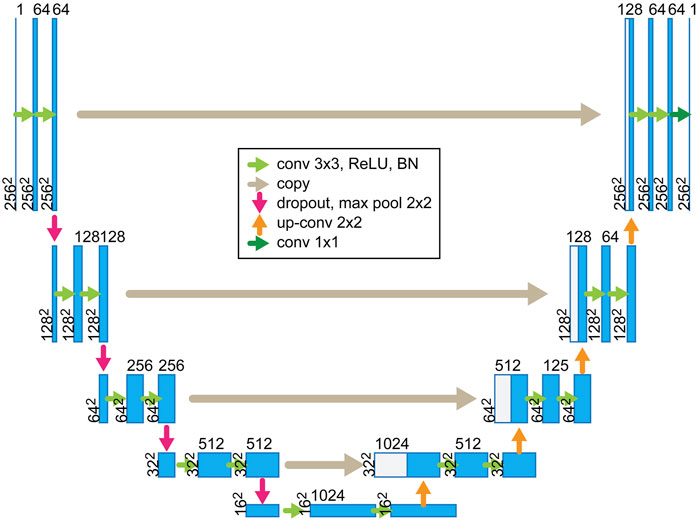
FIGURE 1. Architecture of the convolutional auto-encoder trained for denoising (modified from Ronneberger et al. (2015)). The network consists of an encoder and a decoder. The encoder on the left side compresses inputs into low-dimensional spaces to extract features, and the decoder on the right side uses the features to predict data.

2.3 Parameter optimization

Network parameters are optimized by minimizing misfits between predicted and expected values along the fastest-decreasing direction. We use the Euclidean norm, also known as the L2 norm, to measure the misfit. It is commonly used in geoscience and successfully attenuates noise in many recently published studies (Mandelli et al., 2019; Saad and Chen, 2021). Given the clean signal $x^{*}$ and noisy data $y^{*}$ as defined in Eq. 4, the cost function $C\left(\mathbf{\Theta }\right)$ can be expressed as

$C\left(\mathbf{\Theta }\right)=\frac{1}{n}{\displaystyle \sum }_{i=1}^n{\left(x_i^{*}-y_i^{*}\right)}^2,(5)$

where $n$ is the total sample number of $x^{*}$ and $y^{*}$ in one batch. Then, we backward-propagated the misfit and optimized the parameters in the layers. The updating direction is determined using the adaptive momentum optimization method (Adam) proposed by Kingma and Ba (2014). The Adam method is computationally efficient and requires low memory. In this study, the decay rates ${\beta }_1$ and ${\beta }_2$ were assigned 0.9 and 0.999, respectively, and $ϵ$, the constant value stabilizing the update ratio, is equal to 10^–8.

After completing training, we used the normalized RMSE to quantify the denoising quality. Note that the gain methods were applied during the training. We removed the gain effect before calculating RMSE to fairly evaluate the efficiency of the deep learning-based denoising method using different gain methods. The normalized RMSE is defined as

$\mathrm{n}\mathrm{o}\mathrm{r}\mathrm{m}\mathrm{a}\mathrm{l}\mathrm{i}\mathrm{z}\mathrm{e}\mathrm{d}\mathrm{R}\mathrm{M}\mathrm{S}\mathrm{E}=\sqrt{\frac{{\left(D-d\right)}^2}{D^2}},(6)$

where $D$ and $d$ stand for the clean and denoised data, respectively. A lower value means a better denoising result with the denoised result being closer to clean data.

3 Results and discussion

This section shows the denoising results of synthetic data followed by field data. We first introduced the dataset in each example and then demonstrated the corresponding denoising results. In the synthetic data, input data for training were seismic records calculated using the viscoelastic finite difference algorithm on models built with randomized elastic properties (Bohlen and Saenger, 2006). We showed the denoising results and the limitation test of the trained network. In the field example, we applied the trained network to field seismic data (acquired by the CREWES Project at the University of Calgary) from Hussar, Alberta.

3.1 Synthetic data generation

We built models with randomized elastic properties and calculated the corresponding viscoelastic waveforms using the open-source SOFI2D developed by Bohlen and Saenger (2006). The model parameters are summarized in Table 1, and Figure 2 shows one of the models. The models were 2 km deep and 5 km wide with 1-m grid size in both directions. We first randomly picked 80–160 depths to be the layer bottoms. Each layer was assigned P-wave velocities (V_P), which increased from the shallow to the deep layers, with V_P ranged from 600 m/s to 4,000 m/s. Then, we introduced low-velocity layers and faults into the models, making them more complex. Therefore, 70% of layers had low-velocity layers with velocities 1%–20% lower than their initial velocities; and 30% of the models had a faults dipping 0–5°. To prevent strong reflections near the surface, we smoothed the shallow layers of V_P models. The range of smoothing was decided randomly above a depth between 150 and 300 m. The S-wave velocities (V_S) and densities were later estimated from the V_P models. A V_P/V_S value between 1.7 and 2 was randomly selected for each layer. We used Gardner’s equation to estimate the densities (Gardner et al., 1974). Last, the Q values used to attenuate the seismic amplitude were arbitrarily set at 20, 30, or 40 in each model. The same Q model has no value difference, but different models have individual Q values.

TABLE 1

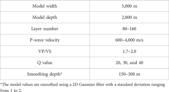
TABLE 1. Model parameters.

FIGURE 2

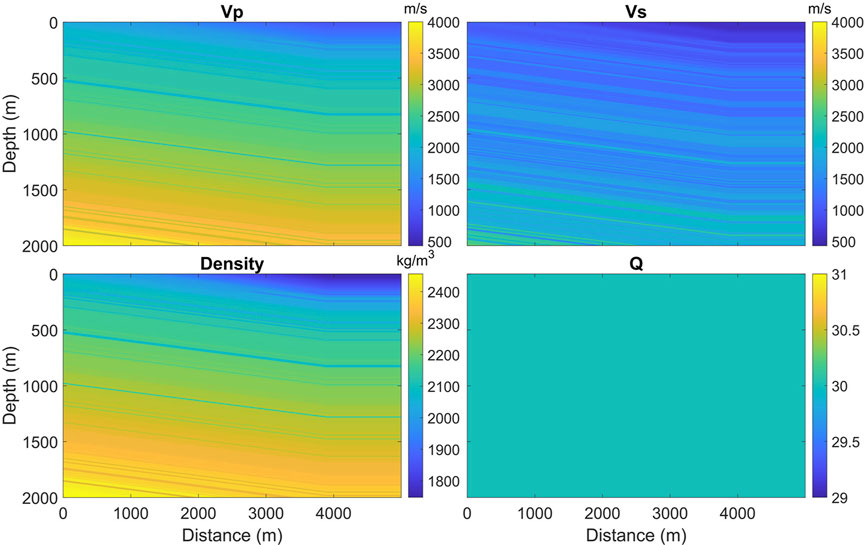
FIGURE 2. Models with randomized elastic properties for viscoelastic waveform modeling. Four properties are needed, including P-wave and S-wave velocities, density, and a seismic quality value that expresses energy attenuation in a media.

Then, the seismic waveforms were calculated, and various noise types were added for training. The receivers were deployed along the free surface with a 10-m spacing. For each model, we forward-calculated a 2-s waveform record. The source location was randomly selected from the receiver locations and had a 50% chance of being a vertical or explosion source. The source wavelets were the Ricker wavelets, with central frequencies arbitrarily chosen from 10 to 20 Hz. When the waveform modeling was completed, we added the following four types of noises to it: 1) high-level Gaussian noise on 0%–20% traces, 2) repetitive hyperbolic noise at fixed locations, 3) random noise generated using Gaussian noise on all traces, and 4) real noise from the field data. The maximum number of repetitive hyperbolic coherent noise we added to the data in one shot gather was 5. Their recurrence frequency is between 5 and 20 Hz, the propagation velocity is between 300 and 800 m/s, and the wavelet is the Ricker wavelet with the central frequency randomly assigned from 5 to 20 Hz. Overall, we generated 1,600 models and their corresponding waveform data pairs—clean and noisy data.

We divided the data into a training set, a validation set, and a test set. In the training set, overfitting almost always occurs if the training time is long enough. Therefore, we stopped iteration once the misfit did not decrease in the validation set and assessed the model’s predictability on the test set. A total of 150 data pairs were randomly selected as the validation or test set, and the remaining 1,300 data were used for the training process.

3.2 Denoising results of synthetic data

The network training was conducted on an NVIDIA V100 GPU and an Intel Xeon CPU. With a learning rate of 10^–3, the learning process was completed within 60 epochs. The learning rate is a tuning parameter that controls the step size of moving toward the minimum of the misfit at each iteration. Within 60 epochs, the misfits of the training and validation datasets sharply decreased before 20 epochs and both turned flat afterward. Please refer to the Supplementary Material to understand in detail how the misfits of the training and validation sets decrease with epochs. Although training 60 epochs took about 27 h to finish, denoising one noisy shot gather via the trained network only needed 60 milliseconds. In practice, instead of inputting an entire shot gather, we did patch-wise training because of GPU memory limitations. We followed Mandelli et al. (2019), segmenting the seismic images into smaller training patches and making them half overlap with adjacent patches in the same image for better denoising efficacy. The patch size was 256-by-256, and the total number of patches for training and validation in one epoch was 15,600 and 1,800, respectively.

3.2.1 Effect of gain settings

The trained U-net successfully denoised the synthetic data. Table 2 shows the average RMSE after denoising decreases from 0.225 to 0.092 and 0.091 for the AGC and the 2D AGC, respectively. One of the clean and noisy (RMSE = 0.29) datasets from the test set and the added noise shown in Figure 3, including two repetitive coherent noises, are located at 2,000 m and 2,650 m, respectively. In the noisy data, the surface waves dominate at the near offset. As offset increases, signal amplitude declines rapidly, and noise gradually dominates, blurring the reflection signals. Therefore, denoising approaches are necessary to improve the coherency of the reflection signals. The denoised results pre-processed by two gain methods are shown in Figure 4 with the AGC applied. The repetitive coherent and other noises, including random noise and dead traces, were generally removed from the noisy data in both results. We will compare traces at their actual values without applying the gain later in zoomed images.

TABLE 2

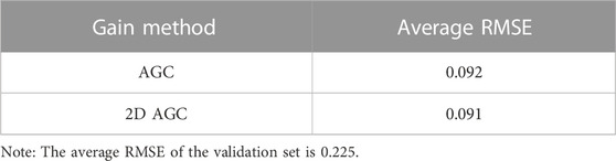
TABLE 2. Influence of the gain settings on denoising performance.

FIGURE 3

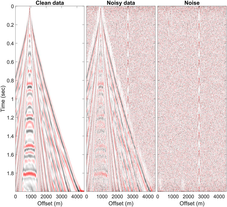
FIGURE 3. Synthetic clean data, noisy data, and the noise are shown with the AGC applied. The noisy data, the superposition of the clean data and the noise, has an RMSE equal to 0.29.

FIGURE 4

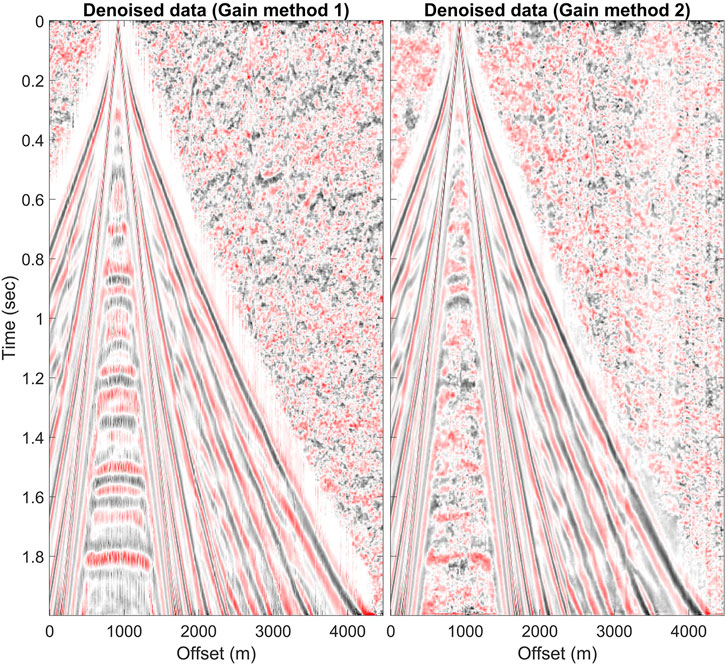
FIGURE 4. Denoising comparison of two gain methods. Images are applied using the AGC. The results using method 1 (the AGC) have an RMSE of 0.09 and those using method 2 (the 2D AGC) have an RMSE of 0.07.

Denoised results depended on the gain settings of the input data, while the noise was generally attenuated. The 2D AGC did not work efficiently at the near offset during training. Figure 5 shows the denoised and desired clean results with the gain methods applied as well as the corresponding residual and removed noises. The residual and removed noise panels are the clean and noisy data subtracted from the denoised data. In Figure 5B, the reflection signals near 1,000 m were indiscernible in the denoised result and the clean data. The 2D AGC uses a moving window to scale traces from their adjacent receivers’ amplitude, which leads to the strong ground roll at the near offset, dramatically lowering the amplitude of the reflection signals. The small amplitude contributes less to the network parameters’ optimization, so the denoising performance is less effective at the near offset. The same situation may also happen near noise strips. Therefore, the window design for the 2D AGC should be carefully considered and has a larger spatial range than the influence range of the strip.

FIGURE 5

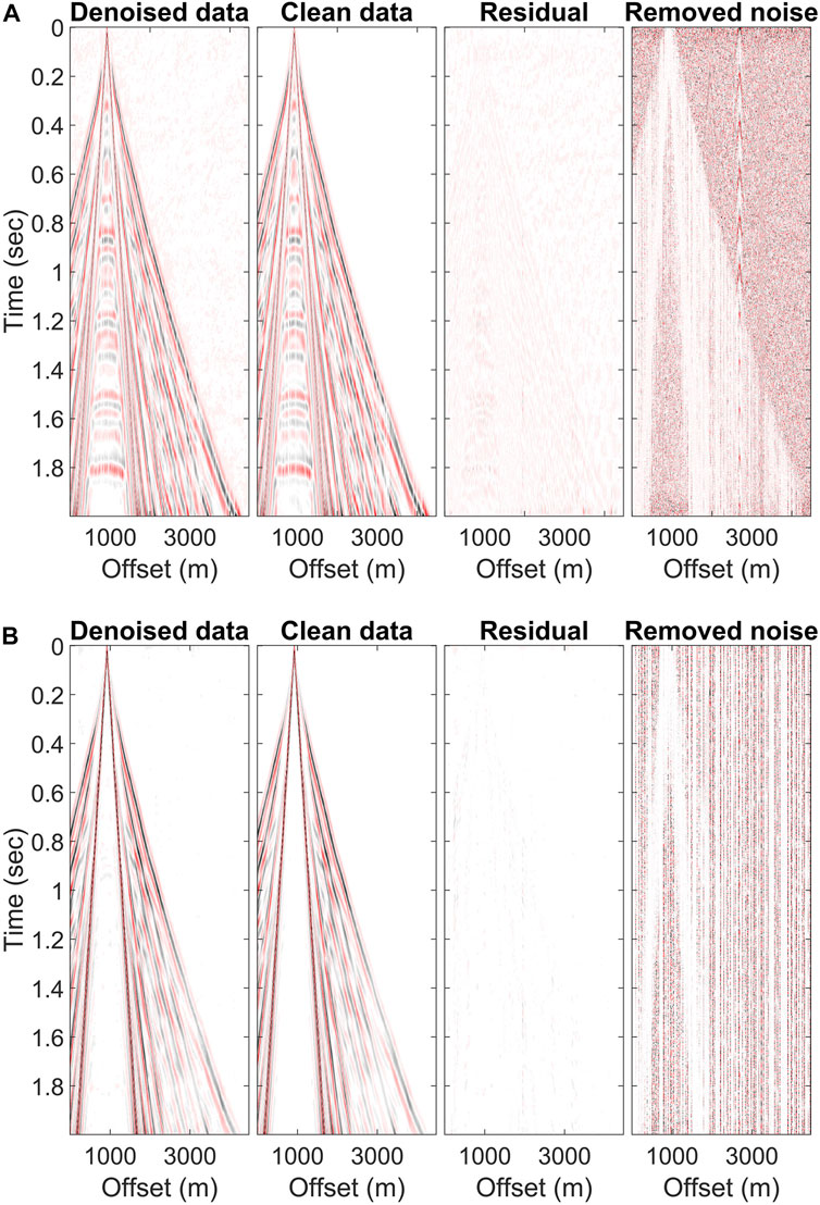
FIGURE 5. Desired clean data and the predicted denoised results in network training with amplitude recovered using the (A) AGC method and (B) 2D AGC method. The residual and the removed noise are, respectively, the clean data and the noisy data subtracted from the denoised results.

Additionally, the general AGC had uneven amplitude in its results. Because the entire shot gather had a wide range of amplitudes, we cropped a section from it with coherent repetitive noise. The zoomed images are shown in Figure 6 in their actual amplitudes. The repetitive, coherent noise was attenuated by the networks using either the AGC or the 2D AGC. The improvement of the signals was clearer when we compared the clean, noisy, and denoised traces. The strongly oscillating noise was suppressed, and the denoised traces of the gain methods 1 and 2 fit well with the clean trace. However, the denoised data pre-processed by gain method 1 have uneven amplitudes between traces, which do not occur in the zoomed images of the clean data and the denoised result gained by method 2.

FIGURE 6

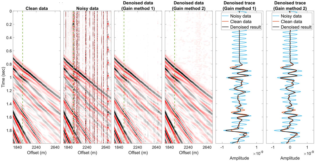
FIGURE 6. Zoomed images of the synthetic data pair and the denoised results. The traces noted as green lines in panels are used to compare denoised results gained by the AGC (method 1) and the proposed 2D AGC (method 2). The trained network using no matter the AGC or the 2D AGC for energy recovery can suppress the strong oscillation noise. However, the denoised result pre-processed by the AGC method has uneven amplitude change that does not exist in the clean data.

Among the two gain methods we used in this study, we preferred the 2D AGC method. While the 2D AGC method did not work efficiently at the near offset, its denoised results have better fidelity with no uneven amplitude between traces. According to the testing results, having uniform amplitudes in seismic gathers is crucial for the network. The uneven amplitude was due to the neglection of adjacent traces’ amplitudes in the AGC method, as shown in Figure 5A. It uses a moving window, scaling the amplitude along the time axis. When traces are contaminated by strong noise during the entire recording time, gain method 1 underperforms because signals are decreased to extremely small values, which makes it difficult for the network to update parameters. On the other hand, the 2D AGC uses a 2D window to scale traces from their adjacent receivers’ amplitudes, so input data for training have a smoother amplitude change. Therefore, we applied the 2D AGC to the field data within a constraint offset range.

3.2.2 Limitation test

We carried out a limitation test of the network before applying it to the real data. The following network was trained using data pre-processed by the 2D AGC because its denoising results had higher fidelity. The deep learning method performs inefficiently if inputs significantly differ from the training set (Yu et al., 2019). However, inputs are never identical to the training set. Their maximum acceptable difference is vague, so we investigated the possible situations when the trained network can directly perform on data and when re-training a network may be needed.

We generated seismic data with a source wavelet and noise types different from the training set to study whether the trained network can denoise successfully. The models for waveform modeling were built as mentioned previously. The source wavelets were the Ricker wavelet with a central frequency of 15 Hz and a sine-cubed wavelet with a central frequency of 30 Hz and a half-period duration. The sine-cubed wavelet of time $f\left(t\right)$ can be expressed as

$f\left(\mathrm{t}\right)=0.75\pi f_C{\sin \left(\pi \left(t\times f_C\right)\right)}^{3}ift\in \left[0,1/f_C\right]elsef\left(t\right)=0.(7)$

In the equation, $\mathrm{t}$ denotes the time and $f_C$ is the central frequency. Then, we added not only the noise types mentioned previously but also linear and spike noises to investigate how the network reacts to noise never trained before. The clean and noisy data with all kinds of noise are shown in Figure 7. To discuss the denoising quality, we zoomed in on the magenta box, as shown in Figure 8.

FIGURE 7

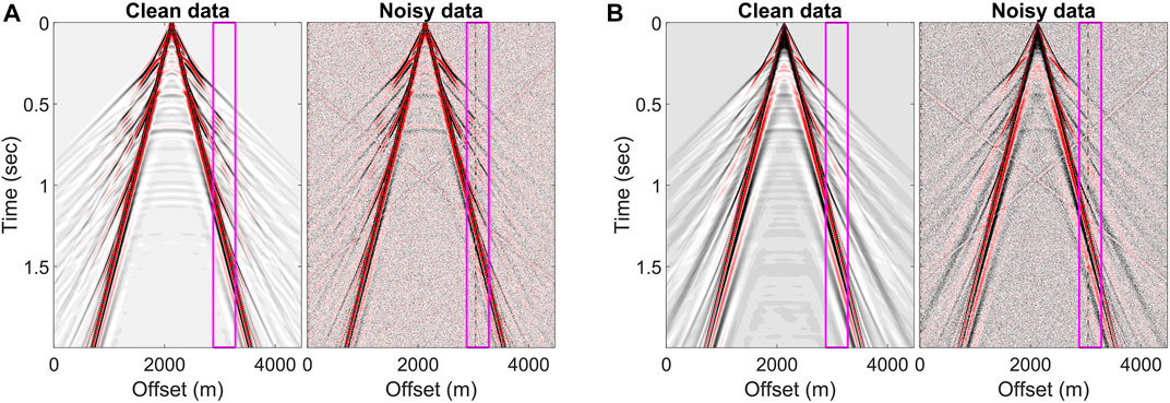
FIGURE 7. Synthetic data pairs for the limitation test. Waveform modeling was calculated using the (A) Ricker wavelet and (B) sine-cubed wavelet. The noise types in noisy data include Gaussian noise, coherent noise in the magenta boxes, three linear noises, and spike noise.

FIGURE 8

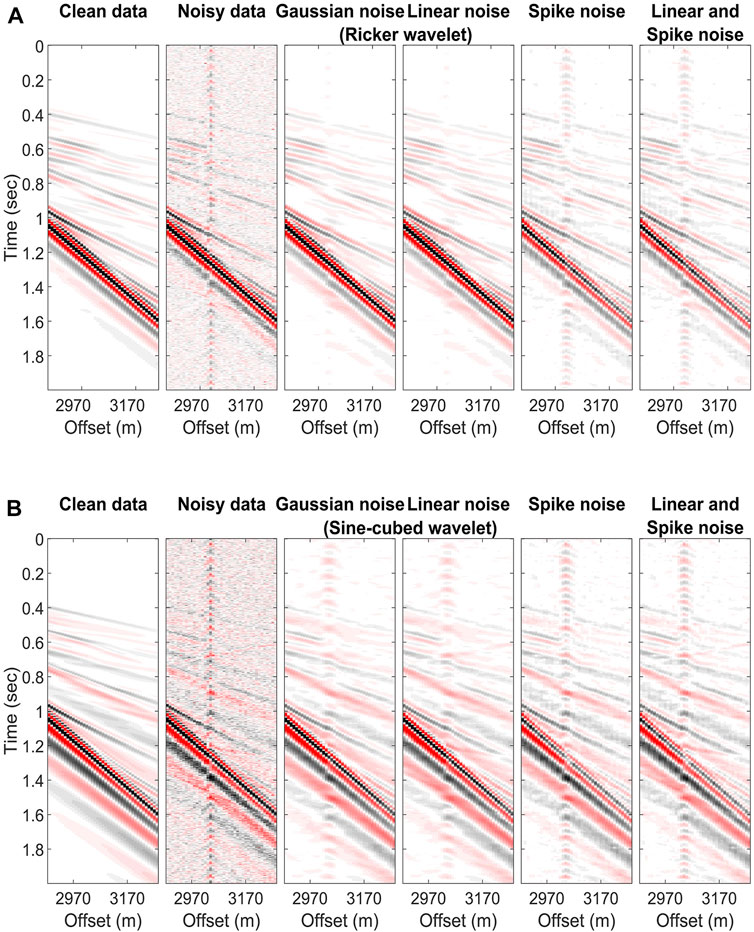
FIGURE 8. Limitation test results with three different noise types and two source wavelets, including the (A) Ricker wavelet and (B) sine-cubed wavelet. The zoomed denoised results are located in the magenta boxes in Figure 7.

Expectably, the denoising network’s performance is relevant to the wavelet and noise types in the training set. Table 3 lists the RMSEs of the noisy data with different noise types and those of the corresponding denoised results. The trained network did not denoise the data modeling with the sine-cubed wavelet no matter what noise was added, as shown in Figure 8B. Although the repetitive coherent noise was attenuated in the noisy data modeling with the Ricker wavelet, the network did not achieve the expected results once the spike noise was included, as shown in Figure 8A. Therefore, we recommend re-training the network if the source wavelet differs from the training set and de-spiking the seismic data before applying the trained network to the data. Depending on the spikes’ character, one can remove them as outliers in the data, directly apply a frequency filter, or use de-spiking algorithms.

TABLE 3

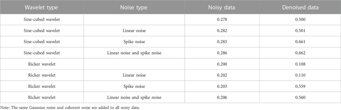
TABLE 3. Denoising performance on different types of noises and wavelet (in terms of RMSE).

3.3 Denoising results of field data

The field dataset was collected in an experimental survey led by the Consortium for Research in Elastic Wave Exploration Seismology (CREWES) at the University of Calgary to investigate the effect of low frequencies on seismic reflections (Margrave et al., 2012). The site is situated near Hussar, Alberta. Dynamite and two different vibroseis sources were tested with five different receiver types. Among them, we selected the dataset generated by dynamite and recorded using the 10-Hz geophones. A measure of 2 kg of dynamite created the most apparent signals among all sources, and the 10-Hz geophones commonly used in the industry did not introduce instrument noise in the low-frequency range. The seismic line is 4.5 km long with a rolling source and fixed receivers spaced 20 m and 10 m, respectively.

The seismic reflection methods use reflectors at different subsurfaces to image the underground structure. The reflection signals have hyperbolic patterns in the time-offset domain and can represent the locations of the subsurfaces after the move out correction and the stacking process. However, in our dataset, noise, including ground roll, pumpjack noise, and noise due to human activity, seriously contaminates the reflection signals, as shown in Figure 9A. Therefore, we aimed to preserve reflection signals while attenuating different types of noise. The processing flow is shown in Figure 10. Noise suppression is applied after the geometry setup and static correction. We used the radial filter to attenuate ground roll and the noise of pumpjack and human activity because radial filtering effectively reduces the noise with a specific velocity at specific frequency band levels (Henley, 2003; Saeed et al., 2014). Subsequently, we sequentially removed shot and receiver effects, compensated for energy loss, and improved temporal resolution. After velocity analysis, we applied surface-consistent residual statics and trim statics to improve the continuity of the reflection signals in the final profile. Last, we used FX deconvolution to suppress random noise.

FIGURE 9

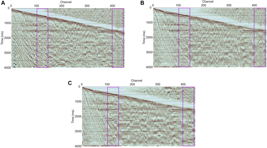
FIGURE 9. (A) Example of field data in a shot gather and the corresponding denoising results of (B) the processing flow and (C) the flow with the U-net denoising step. Two magenta boxes indicate the locations of the pumpjack noise.

FIGURE 10

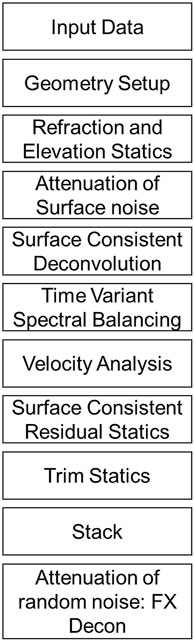
FIGURE 10. Processing flow.

The signal improvement in the field data is hardly quantified as we carried out for the synthetic data because the noise-free seismic data in the field are never known. Instead, we qualitatively evaluated the field data’s improvement by comparing the coherency improvement of reflection signals in different domains. Raw data (Figures 9A, 11A) and denoising results are shown in shot gathers and CMP gathers with and without the trained U-net applied. The corresponding final seismic profiles are shown in Figure 12. The pumpjack noise and ground roll were suppressed by radial filtering, as shown in Figures 9B, 11B. The pumpjack noise initially masked some hyperbolic reflection signals in the raw data (magenta boxes in Figures 9, 11). After radial filtering was applied, the reflection signals had better continuity along their hyperbola. Hence, we expected that the filtered reflection signals on the final seismic profile had been improved. However, some flat noise remained. It is because the frequency range of the noise and the signal overlap. We tried replacing the radial filtering with the curvelet-based filtering in the flow, but the flat noise remained. Additionally, we expected that the noise can be suppressed after the deconvolution because the wavelets of the source and the noise are different; however, the noise is still apparent after processing. On the other hand, the reflection signals were more coherent if we used the U-net to denoise the data. Figure 9C shows the denoised results with the U-net applied in a shot gather. The pumpjack and random noises were suppressed successfully. No flat noise is seen in the gather. The better denoising performance of the U-net is also seen in the CMP domain, as shown in Figure 11C. With the U-net applied, the reflection signals initially masked by the pumpjack noise had better coherency in the CMP gather than without the U-net shown in Figure 11B. In final seismic profiles, as shown in Figure 12, the difference between with and without the U-net denoising applied is clear at the deeper layers. Below 2,000 m, the profile with the U-net applied has clear reflectors and fewer vertical discontinuities caused by the pumpjack noise.

FIGURE 11

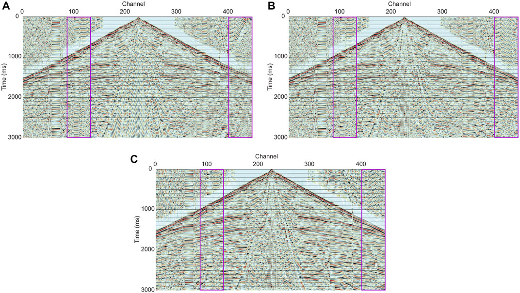
FIGURE 11. (A) Example of field data in a CMP gather and the corresponding denoising results of (B) the processing flow and (C) the flow with the U-net denoising step. Two magenta boxes indicate the locations of the pumpjack noise. The traditional processing flow can improve the continuity of the reflection signals contaminated by the pumpjack noise; because the frequency range of the signal and noise overlap, some flat noise remains. However, if the U-net denoising step is applied, the flat noise does not exist.

FIGURE 12

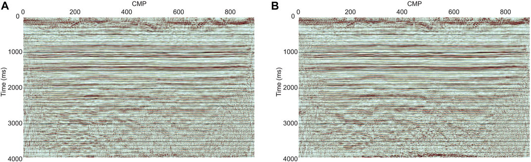
FIGURE 12. Seismic reflection images (A) without and (B) with the trained U-net applied in the processing flow. With the U-net denoising step included in the processing flow, the seismic reflection image is clearer below 2000 m and less affected by the pumpjack noise. Between 200 and 400 CMP, some vertical discontinuities caused by the pumpjack noise are suppressed by the U-net method.

4 Conclusion

We used a deep learning technique (U-net) to suppress coherent noise in seismic shot gathers. Our results indicate that U-nets can be effective at seismic noise attenuation. Gaining the seismic amplitudes prior to noise attenuation is necessary and influences the final denoising quality. We found that using a 2D AGC method to scale amplitude is effective. The performance of the trained network heavily depends on the training dataset. Before applying the trained network to the field data, we tested the denoising performance of the trained network on data with noise different from the training set. Re-training of the noise reduction process may be required if the training data significantly differs from the actual data.

Repetitive coherent noise is difficult to suppress by traditional methods, which require noticeable differences between signals and noise. However, the neural network extracted noise features during training and successfully attenuated noise without detailed geophysical assumptions. Compared with the processing flow with radial filtering and deconvolution, the U-net improved the noise suppression and showed promise as another tool in our signal enhancement kit.

Data availability statement

The raw data supporting the conclusion of this article will be made available by the authors, without undue reservation.

Author contributions

Both authors contributed equally to the research and critically discussed the results. Y-TW finished the analysis and drafted the manuscript. RS commented on and reviewed the manuscript.

Acknowledgments

The authors are grateful to the Hewlett Packard Enterprise Data Science Institute at the University of Houston for providing computing resources. The support from the Department of Earth and Atmospheric Sciences at the University of Houston is much appreciated.

Conflict of interest

The authors declare that the research was conducted in the absence of any commercial or financial relationships that could be construed as a potential conflict of interest.

Publisher’s note

All claims expressed in this article are solely those of the authors and do not necessarily represent those of their affiliated organizations, or those of the publisher, the editors, and the reviewers. Any product that may be evaluated in this article, or claim that may be made by its manufacturer, is not guaranteed or endorsed by the publisher.

Supplementary material

The Supplementary Material for this article can be found online at: https://www.frontiersin.org/articles/10.3389/feart.2023.1082435/full#supplementary-material

References

Bohlen, T., and Saenger, E. H. (2006). Accuracy of heterogeneous staggered-grid finite-difference modeling of Rayleigh waves. Geophysics 71, 109–115. doi:10.1190/1.2213051

CrossRef Full Text | Google Scholar

Cai, A., and Zelt, C. A. (2019). Data weighted full-waveform inversion with adaptive moment estimation for near-surface seismic refraction data. Seg. Tech. Program Expand. Abstr. 54, 2858–2862. doi:10.1190/segam2019-3216353.1

CrossRef Full Text | Google Scholar

Calvert, A. J. (2004). A method for avoiding artifacts in the migration of deep seismic reflection data. Tectonophysics 388, 201–212. doi:10.1016/j.tecto.2004.07.026

CrossRef Full Text | Google Scholar

Canales, L. L. (1984). Random noise reduction. Seg. Tech. Program Expand. Abstr. 856, 525–527. doi:10.1190/1.1894168

CrossRef Full Text | Google Scholar

Chopra, S., and Marfurt, K. J. (2014). Causes and appearance of noise in seismic data volumes. AAPG Explor. 35, 52–55.

Google Scholar

Gardner, G., Gardner, L., and Gregory, A. (1974). Formation velocity and density—the diagnostic basics for stratigraphic traps. Geophysics 39, 770–780. doi:10.1190/1.1440465

CrossRef Full Text | Google Scholar

Goki, S. (2016). Deep running starting from the bottom. Tokyo: O'Reilly Japan. https://www.amazon.com/Deep-running-starting-bottom-Korean/dp/8968484635/ref=sr_1_1?qid=1675299429&refinements=p_27%3ADog+front+map&s=books&sr=1-1.

Google Scholar

Henley, D. (2009). A convenient truth: Radial trace filtering—simple and effective. CSEG Rec. 34, 16–26.

Google Scholar

Henley, D. C. (2003). Coherent noise attenuation in the radial trace domain. Geophysics 68, 1408–1416. doi:10.1190/1.1598134

CrossRef Full Text | Google Scholar

Kingma, D. P., and Ba, J. (2014). Adam: A method for stochastic optimization. arXiv preprint arXiv 1412.6980.

Google Scholar

Klochikhina, E., Crawley, S., Frolov, S., Chemingui, N., and Martin, T. (2020). Leveraging deep learning for seismic image denoising. First Break 38, 41–48. doi:10.3997/1365-2397.fb2020048

CrossRef Full Text | Google Scholar

Kumar, D., and Ahmed, I. (2021). Encyclopedia of Solid Earth Geophysics. Springer. doi:10.1007/978-3-030-58631-7_146 https://link.springer.com/referenceworkentry/10.1007/978-3-030-58631-7_146#citeas.

CrossRef Full Text | Google Scholar

Liu, B., Yue, J., Zuo, Z., Xu, X., Fu, C., Yang, S., et al. (2021). Unsupervised deep learning for random noise attenuation of seismic data. IEEE Geoscience Remote Sens. Lett. 19, 1–5. doi:10.1109/LGRS.2021.3057631

CrossRef Full Text | Google Scholar

Liu, W., Cao, S., Chen, Y., and Zu, S. (2016). An effective approach to attenuate random noise based on compressive sensing and curvelet transform. J. Geophys. Eng. 13, 135–145. doi:10.1088/1742-2132/13/2/135

CrossRef Full Text | Google Scholar

Liu, Y., Liu, C., and Wang, D. (2009). A 1D time-varying median filter for seismic random, spike-like noise elimination. Geophysics 74, 17–24. doi:10.1190/1.3043446

CrossRef Full Text | Google Scholar

Mandelli, S., Lipari, V., Bestagini, P., and Tubaro, S. (2019). Interpolation and denoising of seismic data using convolutional neural networks. arXiv preprint arXiv 1901.07927.

Google Scholar

Margrave, G. F., Mewhort, L., Phillips, T., Hall, M., Bertram, M. B., Lawton, D. C., et al. (2012). The Hussar low-frequency experiment. CSEG Rec. 37, 25–39.

Google Scholar

Onajite, E. (2013). Seismic data analysis techniques in hydrocarbon exploration. Elsevier. https://www.elsevier.com/books/seismic-data-analysis-techniques-in-hydrocarbon-exploration/onajite/978-0-12-420023-4.

Google Scholar

Ronneberger, O., Fischer, P., and Brox, T. (2015). “U-net: Convolutional networks for biomedical image segmentation,” in International Conference on Medical image computing and computer-assisted intervention (Springer), 234–241. https://link.springer.com/chapter/10.1007/978-3-319-24574-4_28.

CrossRef Full Text | Google Scholar

Saad, O. M., and Chen, Y. (2021). A fully unsupervised and highly generalized deep learning approach for random noise suppression. Geophys. Prospect. 69, 709–726. doi:10.1111/1365-2478.13062

CrossRef Full Text | Google Scholar

Saad, O. M., and Chen, Y. (2020). Deep denoising autoencoder for seismic random noise attenuation. Geophysics 85, 367–376. doi:10.1190/geo2019-0468.1

CrossRef Full Text | Google Scholar

Saeed, A. N., Margrave, G. F., Henley, D. C., Isaac, J. H., and Lines, L. R. (2014). Seismic imaging of the Hussar low frequency seismic data. CREWES Res. Rep. 26, 1–18.

Google Scholar

Soubaras, R. (1994). Signal-preserving random noise attenuation by the fx projection SEG Technical Program. Society of Exploration Geophysicists. doi:10.1190/1.1822843 https://library.seg.org/doi/10.1190/1.1822843.

CrossRef Full Text | Google Scholar

Stewart, R. R. (1985). Median filtering: Review and a new F/K analogue design. J. Can. Soc. Explor. Geophys. 21, 54–63.

Google Scholar

Sun, J., Hou, S., Vinje, V., Poole, G., and Gelius, L. J. (2022). Deep learning-based shot-domain seismic deblending. Geophysics 87, V215–V226. doi:10.1190/geo2020-0865.1

CrossRef Full Text | Google Scholar

Tian, C., Fei, L., Zheng, W., Xu, Y., Zuo, W., and Lin, C. W. (2020). Deep learning on image denoising: An overview. Neural Netw. 131, 251–275. doi:10.1016/j.neunet.2020.07.025

PubMed Abstract | CrossRef Full Text | Google Scholar

Trad, D., Ulrych, T., and Sacchi, M. (2003). Latest views of the sparse Radon transform. Geophysics 68, 386–399. doi:10.1190/1.1543224

CrossRef Full Text | Google Scholar

Wang, F., and Chen, S. (2019). Residual learning of deep convolutional neural network for seismic random noise attenuation. IEEE Geoscience Remote Sens. Lett. 16, 1314–1318. doi:10.1109/LGRS.2019.2895702

CrossRef Full Text | Google Scholar

Wang, S., Li, Y., Wu, N., Zhao, Y., and Yao, H. (2020). Attribute-based double constraint denoising network for seismic data. IEEE Trans. Geoscience Remote Sens. 59, 5304–5316. doi:10.1109/TGRS.2020.3021492

CrossRef Full Text | Google Scholar

Yu, S., Ma, J., and Wang, W. (2019). Deep learning for denoising. Geophysics 84, 333–350. doi:10.1190/geo2018-0668.1

CrossRef Full Text | Google Scholar

Zhang, M., Liu, Y., and Chen, Y. (2019). Unsupervised seismic random noise attenuation based on deep convolutional neural network. IEEE Access 7, 179810–179822. doi:10.1109/ACCESS.2019.2959238

CrossRef Full Text | Google Scholar

Zhong, T., Cheng, M., Dong, X., and Wu, N. (2021). Seismic random noise attenuation by applying multiscale denoising convolutional neural network. IEEE Trans. Geoscience Remote Sens. 60, 1–13. doi:10.1109/TGRS.2021.3095922

CrossRef Full Text | Google Scholar

Zhou, H. W. (2014). Practical seismic data analysis. Cambridge University Press. https://www.cambridge.org/highereducation/books/practical-seismic-data-analysis/CBDD7DF03CCA213BF6CFD8152A0F13FE#overview.

Google Scholar