Three-dimensional elastic reverse-time migration using a high-order temporal and spatial staggered-grid finite-difference scheme

Three-dimensional (3D) elastic reverse-time migration (ERTM) can image the subsurface 3D seismic structures, and it is an important tool for the Earth’s interior imaging. A common simulation kernel used in 3D ERTM is the current staggered-grid finite-difference (SGFD) method of the first-order elastic wave equation. However, the mere second-order accuracy in time of the current SGFD method can bring non-negligible time dispersion, which reduces the simulation accuracy and further leads to the distortion of the imaging results. This paper proposes a vector-based 3D ERTM using the high-order accuracy SGFD method in time to obtain high-accuracy images. This approach is a new high-resolution ERTM workflow that improves the imaging accuracy of conventional ERTM from numerical simulation. The proposed ERTM workflow is established on a quasi-stress–velocity wave equation and its vector wavefield decomposition form. Advanced SGFD schemes and their corresponding coefficients with fourth-order temporal accuracy solve the quasi-linear wave equation system. The normalized dot product imaging condition produces high-quality images using high-accuracy vector wavefields solved using the SGFD method. Through the numerical examples, we test the simulation efficiency and analyze how temporal accuracy in numerical simulations affects migration imaging quality. We include that the proposed method obtains highly accurate images.

Introduction

Seismic migration can convert the collected seismic data into the attribute images of the Earth’s interior medium, being a benefit for structure characterization and lithology identification. In contrast to ray-based migration (Bleistein, 1987; Zhang et al., 2019), wave equation migration exploits the kinematics and dynamics of seismic data to generate high-precision images (Claerbout and Doherty, 1972; Gazdag, 1978). Based on the two-way wave equation simulation, reverse-time migration (RTM) uses primary reflections to generate the Earth’s structural image, and it also presents no dip limitations (McMechan, 1983; Whitmore, 1983).

Elastic RTM (ERTM; Chang and McMechan, 1987; Li and Li, 2022) has attracted the interest of researchers in the academic research and exploration industry in the past years due to the rapid development of multicomponent acquisitions, which can record the rich P and S waves in multicomponent seismic data. P and S waves can reflect the elastic nature of the Earth media and both of them have their own advantages in specific geological conditions. By making full use of these two types of waves, ERTM can reveal the multicomponent images (PP, PS, SP, and SS) for our understanding of the elastic properties of the subsurface (Stewart et al., 2003). Compared with two-dimensional ERTM, three-dimensional (3D) ERTM (Du Q. et al., 2014) does not need to make any assumptions about the spatial patterns of geological bodies and has the advantage of making diffraction migration. Therefore, 3D ERTM is an indispensable means to solve structural lithology problems in complex areas. 3D ERTM consists of three main steps: source wavefield forward simulation, receiver data backward simulation and imaging condition application. The first two respects are solving the wave equation, which occupies the foundation of the whole migration. We next review the two main aspects, namely numerical simulation and imaging conditions.

The velocity–stress wave equation of 3D ERTM is solved using the staggered-grid finite-difference (SGFD) method (Virieux, 1986; Wu et al., 2022) in the time domain due to its high efficiency and easy implementation. However, the discretization of partial derivatives using the SGFD method causes truncation errors. The current SGFD method in the literature for 3D ERTM has arbitrary even-order spatial accuracy but low second-order temporal accuracy (Kristek et al., 2010; Zhou et al., 2021b). Although a relatively small discrete time-step can get a relatively accurate wavefield solution, the computational efficiency is very low for a large number of time-step loops. Instead, the computational efficiency can be improved several times when a larger discrete time-step under the constraints of the Courant–Friedrichs–Lewy (CFL, Courant et al., 1928; Zhou et al., 2021a); however, the temporal dispersion problem will be exposed. The low temporal modeling precision causes a severe temporal dispersion through waveform distortion and a phase advance (Wang and Xu, 2015). Such temporal dispersions are numerical errors produced by simulation tools and are independent of the subsurface medium’s properties. Therefore, these errors only occur at the numerical stage and affect the image quality.

More time slices in the calculation or fully spectral methods (Etgen and Brandsberg-Dahl, 2009; Alkhalifah, 2013; Wu and Alkhalifah, 2014) can improve the temporal accuracy when taking the derivative of time, but they have large memory requirements and slow computational efficiency, especially for 3D ERTM. Numerous methods have been proposed to improve the wavefield simulation, such as the high-order time discretization (Chen, 2007), rapid expansion method (Tessmer, 2011), correction approaches by filter and interpolation (Du X. et al., 2014; Li et al., 2016; Koene et al., 2018), low-rank method (Song et al., 2013), and recursive time evolution method (Kosloff et al., 1989; Pestana and Stoffa, 2010). One general concept for better approximating temporal derivatives via the SGFD schemes is incorporating off-axis grid nodes (Tan and Huang, 2014; Chen et al., 2016a; Ren et al., 2017; Ren and Li, 2019; Xu et al., 2019; Zhou et al., 2021a) in calculating spatial derivatives to achieve high-order temporal accuracy. Following the SGFD method, ERTM proposed in this paper introduces a 3D quasi-stress–velocity elastic-wave-based (Chen et al., 2016b) modeling method using SGFD stencils with analytical fourth-order temporal accuracy.

Imaging condition is crucial for elastic wave imaging. Vector-based imaging conditions can generate separate PP, PS, SS, and SP images and can avoid the polarity reversal problem for PS and SP images by the dot-product operator. The wave-mode decomposition is essential to vector-based imaging. Divergence and curl operator-based decoupling of P- and S-wave fields is critical for isotropic media (Yan and Sava, 2008; Yang et al., 2018a). However, the spatial derivative operations in the divergence and curl operators cause phase shifts and amplitude changes in the original wavefield. A vector wavefield decomposition method (Zhang and McMechan, 2010; Yong et al., 2016; Zhu, 2017; Wang et al., 2018; Shi et al., 2019) preserves the vector components in the decomposed P and S waves without changing the phase and amplitude.

As the kind of vector-based imaging condition, the normalized dot-product imaging removes the polarization angle’s amplitude effects (Wang et al., 2016; Du et al., 2017; Yang et al., 2018b). However, it is challenging to accurately estimate the propagation direction and polarity when multiple waves intersect in complex structure areas. Simplified imaging conditions were proposed by retaining the signs of the dot product and recomputing the amplitudes using the absolute value multiplication (Yang et al., 2018b). Following the idea of vector-based wavefield decomposition and simplified imaging conditions, we establish the imaging condition by the wavefields solved from the P- and S-wave decoupled form based on the quasi-stress–velocity wave equation by the temporal high-order SGFD method in this study.

Though full-waveform inversion using SGFD with the high-order accuracy in time has been proposed (Fang et al., 2020; 2021; Ren et al., 2021), 3D ERTM with a temporal high-order SGFD method has not been reported. We take our previous numerical simulation and migration imaging work (Chen et al., 2016b; Fang et al., 2022a) a step further toward the 3D ERTM workflow, improving parts such as source and receiver wavefield simulation, wavefield reconstruction, and MPI parallelism using GPUs (Fang et al., 2022b). We develop a high-accuracy 3D ERTM workflow based on a P/S decoupled quasi-stress–velocity elastic equation, solved by using the SGFD method with high-order accuracy in time and space. With the proposed method, we also investigate how temporal accuracy in numerical simulations affects migration imaging quality. The contributions of this work are to help readers learn about the temporal dispersion effects on ERTM images, and introduce a new high-accuracy imaging 3D ERTM workflow to achieve antidispersion migration imaging. The point of view of improving imaging accuracy from the perspective of high-precision simulation proposed in this paper is applicable to most of the current 3D elastic wave migration imaging technologies to promote the practicability of the algorithm, which is of great significance to the development and industrial application of RTM technology.

The remainder of this paper is organized as follows. The theories and methods are provided, including the 3D quasi-stress–velocity elastic wave equation and its P- or S-wavefield decomposition formula, followed by an accurate temporal fourth-order and spatial high-order SGFD method solution. Next, a normalized dot-product imaging condition and corresponding ERTM workflow produce PP and PS images. In the numerical example part, the efficiency and accuracy of wavefield simulation are tested, and two migration examples are presented to illustrate the proposed 3D ERTM workflow’s performance. Finally, discussions are provided, and a conclusion and the importance of the proposed study are provided.

Methods

Wave equation and its decomposition formula

The quasi-stress–velocity elastic wave equation (Chen et al., 2016b) for the 3D is defined as

$\left\{\begin{array}{l}\mathit{\rho }{\partial }_{\mathit{t}}{\mathit{v}}_{\mathit{x}}={\partial }_{\mathit{x}}^{\mathit{\alpha }}{\mathit{\tau }}_{111}+{\partial }_{\mathit{x}}^{\mathit{\beta }}{\mathit{\tau }}_{111\mathit{x}}+{\partial }_{\mathit{y}}^{\mathit{\beta }}{\mathit{\tau }}_{12}+{\partial }_{\mathit{z}}^{\mathit{\beta }}{\mathit{\tau }}_{13}\\ \mathit{\rho }{\partial }_{\mathit{t}}{\mathit{v}}_{\mathit{y}}={\partial }_{\mathit{x}}^{\mathit{\beta }}{\mathit{\tau }}_{12}+{\partial }_{\mathit{y}}^{\mathit{\alpha }}{\mathit{\tau }}_{111}+{\partial }_{\mathit{y}}^{\mathit{\beta }}{\mathit{\tau }}_{111\mathit{y}}+{\partial }_{\mathit{z}}^{\mathit{\beta }}{\mathit{\tau }}_{23}\\ \mathit{\rho }{\partial }_{\mathit{t}}{\mathit{v}}_{\mathit{z}}={\partial }_{\mathit{x}}^{\mathit{\beta }}{\mathit{\tau }}_{13}+{\partial }_{\mathit{y}}^{\mathit{\beta }}{\mathit{\tau }}_{23}+{\partial }_{\mathit{z}}^{\mathit{\alpha }}{\mathit{\tau }}_{111}+{\partial }_{\mathit{z}}^{\mathit{\beta }}{\mathit{\tau }}_{111\mathit{z}}\\ {\partial }_{\mathit{t}}{\mathit{\tau }}_{111}=\left(\mathit{\lambda }+2\mathit{\mu }\right)\left({\partial }_{\mathit{x}}^{\mathit{\alpha }}{\mathit{v}}_{\mathit{x}}+{\partial }_{\mathit{y}}^{\mathit{\alpha }}{\mathit{v}}_{\mathit{y}}+{\partial }_{\mathit{z}}^{\mathit{\alpha }}{\mathit{v}}_{\mathit{z}}\right)\\ {\partial }_{\mathit{t}}{\mathit{\tau }}_{111\mathit{x}}=-2\mathit{\mu }\left({\partial }_{\mathit{y}}^{\mathit{\beta }}{\mathit{v}}_{\mathit{y}}+{\partial }_{\mathit{z}}^{\mathit{\beta }}{\mathit{v}}_{\mathit{z}}\right)\\ {\partial }_{\mathit{t}}{\mathit{\tau }}_{111\mathit{y}}=-2\mathit{\mu }\left({\partial }_{\mathit{x}}^{\mathit{\beta }}{\mathit{v}}_{\mathit{x}}+{\partial }_{\mathit{z}}^{\mathit{\beta }}{\mathit{v}}_{\mathit{z}}\right)\\ {\partial }_{\mathit{t}}{\mathit{\tau }}_{111\mathit{z}}=-2\mathit{\mu }\left({\partial }_{\mathit{x}}^{\mathit{\beta }}{\mathit{v}}_{\mathit{x}}+{\partial }_{\mathit{y}}^{\mathit{\beta }}{\mathit{v}}_{\mathit{y}}\right)\\ {\partial }_{\mathit{t}}{\mathit{\tau }}_{12}=\mathit{\mu }\left({\partial }_{\mathit{x}}^{\mathit{\beta }}{\mathit{v}}_{\mathit{y}}+{\partial }_{\mathit{y}}^{\mathit{\beta }}{\mathit{v}}_{\mathit{x}}\right)\\ {\partial }_{\mathit{t}}{\mathit{\tau }}_{13}=\mathit{\mu }\left({\partial }_{\mathit{x}}^{\mathit{\beta }}{\mathit{v}}_{\mathit{z}}+{\partial }_{\mathit{z}}^{\mathit{\beta }}{\mathit{v}}_{\mathit{x}}\right)\\ {\partial }_{\mathit{t}}{\mathit{\tau }}_{23}=\mathit{\mu }\left({\partial }_{\mathit{y}}^{\mathit{\beta }}{\mathit{v}}_{\mathit{z}}+{\partial }_{\mathit{z}}^{\mathit{\beta }}{\mathit{v}}_{\mathit{y}}\right)\end{array}\right.,(1)$

where $\mathit{\lambda }$ and $\mathit{\mu }$ are the Lamé parameters, $\mathit{\rho }$ is the density; $\mathit{\lambda }+2\mathit{\mu }=\mathit{\rho }{\mathit{\alpha }}^2$, $\mathit{\mu }=\mathit{\rho }{\mathit{\beta }}^2$, $\mathit{\alpha }$ and $\mathit{\beta }$ respectively are the P- and S-wave velocities, ${\mathit{v}}_{\mathit{x}}$, ${\mathit{v}}_{\mathit{y}}$, and ${\mathit{v}}_{\mathit{z}}$ are the particle velocity components, ${\mathit{\tau }}_{111}$, ${\mathit{\tau }}_{111\mathit{x}}$, ${\mathit{\tau }}_{111\mathit{y}}$, and ${\mathit{\tau }}_{111\mathit{z}}$ are the particle normal stress components, where ${\mathit{\tau }}_{111}$ is associated with the P wave, and the rest of the components are associated with the S wave, ${\mathit{\tau }}_{12}$, ${\mathit{\tau }}_{13}$, and ${\mathit{\tau }}_{23}$ are the particle shear stress components relative to the S wave. Compared to the standard first-order elastic equation, we have ${\mathit{\tau }}_{\mathit{x}\mathit{x}}={\mathit{\tau }}_{111}$ + ${\mathit{\tau }}_{111\mathit{x}}$, ${\mathit{\tau }}_{\mathit{y}\mathit{y}}={\mathit{\tau }}_{111}$ + ${\mathit{\tau }}_{111\mathit{y}}$, ${\mathit{\tau }}_{\mathit{z}\mathit{z}}={\mathit{\tau }}_{111}$ + ${\mathit{\tau }}_{111\mathit{z}}$, ${\mathit{\tau }}_{\mathit{x}\mathit{y}}={\mathit{\tau }}_{12}$, ${\mathit{\tau }}_{\mathit{x}\mathit{z}}={\mathit{\tau }}_{13}$, and ${\mathit{\tau }}_{\mathit{y}\mathit{z}}={\mathit{\tau }}_{23}.$ Furthermore, ${\partial }_{\mathit{t}}$ is the first-order temporal differential operator, ${\partial }_{\mathit{r}}\left(\cdot \right)$ and $\left(\mathit{r}=\mathit{x},\mathit{y}or\mathit{z}\right)$ represent the spatial derivatives for $\mathit{r}$.

Each derivative is related to the P- or S-wave velocities from Eq. 1. Therefore, P- and S-wave separation can be achieved during the wave propagation marching. Then, the partial-velocity components in Eq. 1 in P- and S-wave decomposition forms can be rewritten as Eq. 2:

$\left\{\begin{array}{l}\mathit{\rho }{\partial }_{\mathit{t}}{\mathit{v}}_{\mathit{x}}^{\mathit{\beta }}={\partial }_{\mathit{x}}^{\mathit{\beta }}{\mathit{\tau }}_{111\mathit{x}}+{\partial }_{\mathit{y}}^{\mathit{\beta }}{\mathit{\tau }}_{12}+{\partial }_{\mathit{z}}^{\mathit{\beta }}{\mathit{\tau }}_{13}\\ \mathit{\rho }{\partial }_{\mathit{t}}{\mathit{v}}_{\mathit{y}}^{\mathit{\beta }}={\partial }_{\mathit{x}}^{\mathit{\beta }}{\mathit{\tau }}_{12}+{\partial }_{\mathit{y}}^{\mathit{\beta }}{\mathit{\tau }}_{111\mathit{y}}+{\partial }_{\mathit{z}}^{\mathit{\beta }}{\mathit{\tau }}_{23}\\ \mathit{\rho }{\partial }_{\mathit{t}}{\mathit{v}}_{\mathit{z}}^{\mathit{\beta }}={\partial }_{\mathit{x}}^{\mathit{\beta }}{\mathit{\tau }}_{13}+{\partial }_{\mathit{y}}^{\mathit{\beta }}{\mathit{\tau }}_{23}+{\partial }_{\mathit{z}}^{\mathit{\beta }}{\mathit{\tau }}_{111\mathit{z}}\\ \mathit{\rho }{\partial }_{\mathit{t}}{\mathit{v}}_{\mathit{x}}^{\mathit{\alpha }}={\partial }_{\mathit{x}}^{\mathit{\alpha }}{\mathit{\tau }}_{111}\\ \mathit{\rho }{\partial }_{\mathit{t}}{\mathit{v}}_{\mathit{y}}^{\mathit{\alpha }}={\partial }_{\mathit{y}}^{\mathit{\alpha }}{\mathit{\tau }}_{111}\\ \mathit{\rho }{\partial }_{\mathit{t}}{\mathit{v}}_{\mathit{z}}^{\mathit{\alpha }}={\partial }_{\mathit{z}}^{\mathit{\alpha }}{\mathit{\tau }}_{111}\\ {\mathit{v}}_{\mathit{x}}={\mathit{v}}_{\mathit{x}}^{\mathit{\alpha }}+{\mathit{v}}_{\mathit{x}}^{\mathit{\beta }}\\ {\mathit{v}}_{\mathit{y}}={\mathit{v}}_{\mathit{y}}^{\mathit{\alpha }}+{\mathit{v}}_{\mathit{y}}^{\mathit{\beta }}\\ {\mathit{v}}_{\mathit{z}}={\mathit{v}}_{\mathit{z}}^{\mathit{\alpha }}+{\mathit{v}}_{\mathit{z}}^{\mathit{\beta }}\end{array}\right.,(2)$

where ${\mathit{v}}_{\mathit{x}}^{\mathit{\alpha }}$, ${\mathit{v}}_{\mathit{y}}^{\mathit{\alpha }}$, and ${\mathit{v}}_{\mathit{z}}^{\mathit{\alpha }}$ are calculated using the derivatives of ${\partial }_{\mathit{j}}^{\mathit{\alpha }}$ $\left(\mathit{j}=\mathit{x},\mathit{y},\mathit{z}\right)$, which are related to the P-wave velocity and only included in the P waves, whereas ${\mathit{v}}_{\mathit{x}}^{\mathit{\beta }}$, ${\mathit{v}}_{\mathit{y}}^{\mathit{\beta }}$, and ${\mathit{v}}_{\mathit{z}}^{\mathit{\beta }}$ are wavefields related to the S wave. After substituting Eq. 2 into Eq. 1, we have a complete quasi-stress–velocity wave equation of the decoupled P/S wave propagation as

$\left\{\begin{array}{l}\mathit{\rho }{\partial }_{\mathit{t}}{\mathit{v}}_{\mathit{x}}^{\mathit{\alpha }}={\partial }_{\mathit{x}}^{\mathit{\alpha }}{\mathit{\tau }}_{111},\mathit{\rho }{\partial }_{\mathit{t}}{\mathit{v}}_{\mathit{x}}^{\mathit{\beta }}={\partial }_{\mathit{x}}^{\mathit{\beta }}{\mathit{\tau }}_{111\mathit{x}}+{\partial }_{\mathit{y}}^{\mathit{\beta }}{\mathit{\tau }}_{12}+{\partial }_{\mathit{z}}^{\mathit{\beta }}{\mathit{\tau }}_{13}\\ \mathit{\rho }{\partial }_{\mathit{t}}{\mathit{v}}_{\mathit{y}}^{\mathit{\alpha }}={\partial }_{\mathit{y}}^{\mathit{\alpha }}{\mathit{\tau }}_{111},\mathit{\rho }{\partial }_{\mathit{t}}{\mathit{v}}_{\mathit{y}}^{\mathit{\beta }}={\partial }_{\mathit{x}}^{\mathit{\beta }}{\mathit{\tau }}_{12}+{\partial }_{\mathit{y}}^{\mathit{\beta }}{\mathit{\tau }}_{111\mathit{y}}+{\partial }_{\mathit{z}}^{\mathit{\beta }}{\mathit{\tau }}_{23}\\ \mathit{\rho }{\partial }_{\mathit{t}}{\mathit{v}}_{\mathit{z}}^{\mathit{\alpha }}={\partial }_{\mathit{z}}^{\mathit{\alpha }}{\mathit{\tau }}_{111},\mathit{\rho }{\partial }_{\mathit{t}}{\mathit{v}}_{\mathit{z}}^{\mathit{\beta }}={\partial }_{\mathit{x}}^{\mathit{\beta }}{\mathit{\tau }}_{13}+{\partial }_{\mathit{y}}^{\mathit{\beta }}{\mathit{\tau }}_{23}+{\partial }_{\mathit{z}}^{\mathit{\beta }}{\mathit{\tau }}_{111\mathit{z}}\\ {\mathit{v}}_{\mathit{x}}={\mathit{v}}_{\mathit{x}}^{\mathit{\alpha }}+{\mathit{v}}_{\mathit{x}}^{\mathit{\beta }},{\mathit{v}}_{\mathit{y}}={\mathit{v}}_{\mathit{y}}^{\mathit{\alpha }}+{\mathit{v}}_{\mathit{y}}^{\mathit{\beta }},{\mathit{v}}_{\mathit{z}}={\mathit{v}}_{\mathit{z}}^{\mathit{\alpha }}+{\mathit{v}}_{\mathit{z}}^{\mathit{\beta }}\\ {\partial }_{\mathit{t}}{\mathit{\tau }}_{111}=\left(\mathit{\lambda }+2\mathit{\mu }\right)\left({\partial }_{\mathit{x}}^{\mathit{\alpha }}{\mathit{v}}_{\mathit{x}}+{\partial }_{\mathit{y}}^{\mathit{\alpha }}{\mathit{v}}_{\mathit{y}}+{\partial }_{\mathit{z}}^{\mathit{\alpha }}{\mathit{v}}_{\mathit{z}}\right)\\ {\partial }_{\mathit{t}}{\mathit{\tau }}_{111\mathit{x}}=-2\mathit{\mu }\left({\partial }_{\mathit{y}}^{\mathit{\beta }}{\mathit{v}}_{\mathit{y}}+{\partial }_{\mathit{z}}^{\mathit{\beta }}{\mathit{v}}_{\mathit{z}}\right)\\ {\partial }_{\mathit{t}}{\mathit{\tau }}_{111\mathit{y}}=-2\mathit{\mu }\left({\partial }_{\mathit{x}}^{\mathit{\beta }}{\mathit{v}}_{\mathit{x}}+{\partial }_{\mathit{z}}^{\mathit{\beta }}{\mathit{v}}_{\mathit{z}}\right)\\ {\partial }_{\mathit{t}}{\mathit{\tau }}_{111\mathit{z}}=-2\mathit{\mu }\left({\partial }_{\mathit{x}}^{\mathit{\beta }}{\mathit{v}}_{\mathit{x}}+{\partial }_{\mathit{y}}^{\mathit{\beta }}{\mathit{v}}_{\mathit{y}}\right)\\ {\partial }_{\mathit{t}}{\mathit{\tau }}_{12}=\mathit{\mu }\left({\partial }_{\mathit{x}}^{\mathit{\beta }}{\mathit{v}}_{\mathit{y}}+{\partial }_{\mathit{y}}^{\mathit{\beta }}{\mathit{v}}_{\mathit{x}}\right)\\ {\partial }_{\mathit{t}}{\mathit{\tau }}_{13}=\mathit{\mu }\left({\partial }_{\mathit{x}}^{\mathit{\beta }}{\mathit{v}}_{\mathit{z}}+{\partial }_{\mathit{z}}^{\mathit{\beta }}{\mathit{v}}_{\mathit{x}}\right)\\ {\partial }_{\mathit{t}}{\mathit{\tau }}_{23}=\mathit{\mu }\left({\partial }_{\mathit{y}}^{\mathit{\beta }}{\mathit{v}}_{\mathit{z}}+{\partial }_{\mathit{z}}^{\mathit{\beta }}{\mathit{v}}_{\mathit{y}}\right)\end{array}\right..(3)$

It can be observed from Eq. 3 that the P- and S-wave partial velocity components are automatically decoupled at each time step while the interaction between the P- and S-wave is retained during the propagation.

High-accuracy wavefield simulation

This subsection solves the equation system with the decomposition formula (Eq. 3) using a high-order temporal and spatial accuracy SGFD method. The consensus is that the temporal derivative approximation in Eq. 3 only has second-order SGFD accuracy. However, the spatial derivative approximation has an arbitrary even-order by employing on-axis grid values. As we know, improving the temporal accuracy directly, such as using more wavefield time schemes in the temporal derivative approximation, is nearly forbidden for 3D simulation due to the large memory cost of so many wavefield variables. Therefore, an available “k-space” approach (Fomel et al., 2013; Fang et al., 2014; Wu and Alkhalifah, 2014; Chen et al., 2016b) can ease this issue by transferring the temporal accuracy into the spatial derivation implementation. Typically, the off-axis grid values are introduced into the spatial derivative calculation to improve the temporal accuracy based on the k-space method. Then, the high temporal accuracy is determined through the dispersion relation in the spatial derivative calculation.

Let $\mathit{\chi }=\mathit{\alpha }or\mathit{\beta }$. $\mathit{u}$ indicates all wavefield variables. As usual, the solution for ${\partial }_{\mathit{t}}\left(\mathit{u}\right)$ is approximated by the first-order derivatives as,

${\partial }_{\mathit{t}}\left(\mathit{u}\right)\approx \frac{1}{\mathit{\Delta }\mathit{t}}\left[\mathit{u}\left(\mathit{t}+\mathit{\Delta }\mathit{t}\right)-\mathit{u}\left(\mathit{t}\right)\right],(4)$

where Δt denotes the time step. However, the solution for ${\partial }_{\mathit{r}}^{\mathit{\chi }}\left(\mathit{u}\right)$ $\left(\mathit{r}=\mathit{x},\mathit{y}or\mathit{z}\right)$ is achieved using the SGFD stencil (Tan and Huang 2014) defined in Eq. 5.

${\partial }_r^{\chi }u\approx \frac{1}{h_r}\left\{\begin{array}{c}{\sum }_{m=1}^{N_r}{c}_{m,\mathrm{0,0}}^{r,\chi }\left(u_{r+m-0.5}^{\varphi ,\phi }-u_{r-m+0.5}^{\varphi ,\phi }\right)\\ +c_{\mathrm{1,1,0}}^{r\varphi ,\chi }\left(u_{r+0.5}^{\varphi +1,\phi }-u_{r-0.5}^{\varphi +1,\phi }+u_{r+0.5}^{\varphi -1,\phi }-u_{r-0.5}^{\varphi -1,\phi }\right)\\ +c_{\mathrm{1,0,1}}^{r\phi ,\chi }\left(u_{r+0.5}^{\varphi ,\phi +1}-u_{r-0.5}^{\varphi ,\phi +1}+u_{r+0.5}^{\varphi ,\phi -1}-u_{r-0.5}^{\varphi ,\phi -1}\right)\end{array}\right\},(5)$

where $\varphi$ and $\phi$ denote another two coordinate axes different from r; therefore, $r,\varphi ,\phi \in \left(x,y,z\right)$, $r\ne \varphi \ne \phi .$ $h_r$ represents the grid spacing along the $r-\mathrm{a}\mathrm{x}\mathrm{i}\mathrm{s}$, and $N_r$ represents the stencil length on one side. Equation 5 is illustrated in Figure 1, where $2N_r+8$ grids are used to calculate the spatial derivative. Different from traditional stencil, the advanced one includes an extra eight grid points in the spatial derivative approximation.

FIGURE 1

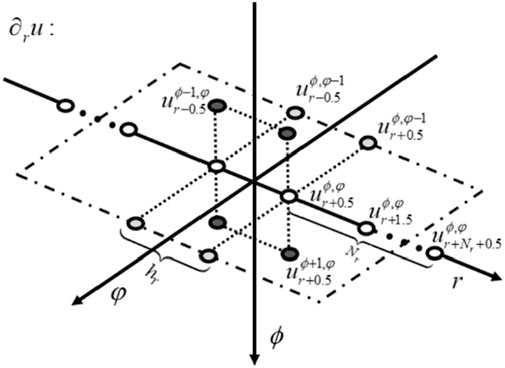
FIGURE 1. Staggered-grid finite-difference (SGFD) stencil of the fourth-order temporal accuracy and arbitrary even-order spatial accuracy, $r,\varphi ,\phi \in \left(x,y,z\right)$ and $r\ne \varphi \ne \phi$.

The dispersion relations in the frequency-wavenumber domain are used to determine the SGFD coefficients. Then the wavenumber response of ${\partial }_{\mathit{r}}^{\mathit{\chi }}\left(\mathit{u}\right)$ and its approximation is derived as

$i{k}_r^{\chi }\approx \frac{2i}{h_r}\left\{\begin{array}{c}{\sum }_{m=1}^{N_r}{c}_{m,\mathrm{0,0}}^{r,\chi }\sin \left(\left(m-0.5\right)k_r{h}_r\right)\\ +2c_{\mathrm{1,1,0}}^{r\varphi ,\chi }\sin \left(\frac{k_r{h}_r}{2}\right)\cos \left(k_{\varphi }{h}_{\varphi }\right)\\ +2c_{\mathrm{1,0,1}}^{r\phi ,\chi }\sin \left(\frac{k_r{h}_r}{2}\right)\cos \left(k_{\phi }{h}_{\phi }\right)\end{array}\right\},(6)$

The SGFD stencil’s Fourier responses can compensate for temporal and spatial dispersion errors using suitable SGFD coefficients. Following the idea of Tan and Huang (2014) and Chen et al. (2016b) of attaining SGFD coefficients, we match the Fourier response of the SGFD discretized Laplacian and velocity-dependent second-order k-space operator, as

$\mathrm{F}\left({\partial }_{tt}u\right)={\chi }^2\left[{\left.{\left(ik\right.}_x^{\chi }\right)}^2+{\left.{\left(ik\right.}_y^{\chi }\right)}^2+{\left.{\left(ik\right.}_z^{\chi }\right)}^2\right],(7)$

where F denotes the Fourier transform. By substituting Eq. 6 into Eq. 7, we have,

$\begin{array}{c}{\gamma }_{x,\chi }^2{\left\{{\displaystyle \sum }_{m=1}^{N_x}{c}_{m,0,0}^{x,\chi }\sin \left[\left(m-\frac{1}{2}\right)k_x{h}_x\right]+2c_{1,1,0}^{xy,\chi }\sin \left(\frac{1}{2}{k}_x{h}_x\right)\cos \left(k_y{h}_y\right)+2c_{1,0,1}^{xz,\chi }\sin \left(\frac{1}{2}{k}_x{h}_x\right)\cos \left(k_z{h}_z\right)\right\}}^2\\ +{\gamma }_{y,\chi }^2{\left\{{\displaystyle \sum }_{m=1}^{N_y}{c}_{m,0,0}^{y,\chi }\sin \left[\left(m-\frac{1}{2}\right)k_y{h}_y\right]+2c_{1,1,0}^{yx,\chi }\sin \left(\frac{1}{2}{k}_y{h}_y\right)\cos \left(k_x{h}_x\right)+2c_{1,0,1}^{yz,\chi }\sin \left(\frac{1}{2}{k}_y{h}_y\right)\cos \left(k_z{h}_z\right)\right\}}^2\\ +{\gamma }_{z,\chi }^2{\left\{{\displaystyle \sum }_{m=1}^{N_z}{c}_{m,0,0}^{z,\chi }\sin \left[\left(m-\frac{1}{2}\right)k_z{h}_z\right]+2c_{1,1,0}^{zx,\chi }\sin \left(\frac{1}{2}{k}_z{h}_z\right)\cos \left(k_x{h}_x\right)+2c_{1,0,1}^{zy,\chi }\sin \left(\frac{1}{2}{k}_z{h}_z\right)\cos \left(k_y{h}_y\right)\right\}}^2+\\ =\frac{1}{2}\left[1-\cos \left(\chi \mathit{\Delta }tk\right)\right],\end{array}(8)$

where ${\gamma }_{r,\chi }=\chi \mathit{\Delta }t/h_r\left(r=x,y\mathrm{o}\mathrm{r}z\right)$ denotes the velocity-dependent CFL number, and the wavenumber $k=\sqrt{k_x^2+k_y^2+k_z^2}$.

After applying the Taylor series expansion to the trigonometric function in Eq. 8, we make the coefficients of the terms ${\mathit{h}}_{\mathit{x}}^{2\mathit{j}}$, ${\mathit{h}}_{\mathit{y}}^{2\mathit{j}}$ and ${\mathit{h}}_{\mathit{z}}^{2\mathit{j}}$ $\left(\mathit{j}=1,2,\dots ,{\mathit{N}}_{\mathit{r}}and{\mathit{N}}_{\mathit{r}}={\mathit{N}}_{\mathit{x}},{\mathit{N}}_{\mathit{y}}or{\mathit{N}}_{\mathit{z}}\right)$ the same on the sides of the equation to achieve the ${2\mathit{N}}_{\mathit{r}}$ order SGFD accuracy in space. Similarly, the coefficients of the hybrid terms ${\mathit{h}}_{\mathit{x}}^2{\mathit{h}}_{\mathit{y}}^2$, ${\mathit{h}}_{\mathit{x}}^2{\mathit{h}}_{\mathit{z}}^2$ and ${\mathit{h}}_{\mathit{y}}^2{\mathit{h}}_{\mathit{z}}^2$ are equalized to the coefficients of $\mathit{\Delta }{\mathit{t}}^4$ on the other side of the equation to attain the fourth-order temporal accuracy. Due to the above strict constraints, the truncation error is $\mathit{o}\left({\mathit{h}}_{\mathit{r}}^{2{\mathit{N}}_{\mathit{r}}}\right)+\mathit{o}\left(\mathit{\Delta }{\mathit{t}}^4\right)$ derived from the dispersion relationship based on the SGFD stencil; therefore, the SGFD simulation’s accuracy could be any even-order (2N_r) in space and the fourth-order in time (2Nr, 4). The SGFD coefficients ${\mathit{c}}_{\mathit{m},\mathrm{0,0}}^{\mathit{r},\mathit{\chi }}\left(\mathit{m}\in \left[1,{\mathit{N}}_{\mathit{r}}\right],\mathit{m}\in {\mathit{Z}}^{+}\right)$, ${\mathit{c}}_{\mathrm{1,1,0}}^{\mathit{r}\mathit{\varphi },\mathit{\chi }}$, and ${\mathit{c}}_{\mathrm{1,0,1}}^{\mathit{r}\mathit{\phi },\mathit{\chi }}$ related to the SGFD stencil are expressed in Eq. 9.

$\left\{\begin{array}{l}{c}_{\mathrm{1,1,0}}^{r\varphi ,\chi }=\frac{1}{24}{\gamma }_{\varphi ,\chi }^2,c_{\mathrm{1,0,1}}^{r\phi ,\chi }=\frac{1}{24}{\gamma }_{\phi ,\chi }^2\\ c_{m,\mathrm{0,0}}^{r,\chi }=\frac{{\left(-1\right)}^{m+1}}{2m-1}{\sum }_{l=1,l\ne m}^{N_r}\frac{{\left(2l-1\right)}^2-{\gamma }_{r,\chi }^2}{\left|{\left(2m-1\right)}^2-{\left(2l-1\right)}^2\right|},\left(m=\mathrm{2,3},\cdots ,N_r\right)\\ c_{\mathrm{1,0,0}}^{r,\chi }=1-2c_{\mathrm{1,1,0}}^{r\varphi ,\chi }-2c_{\mathrm{1,0,1}}^{r\phi ,\chi }-{\sum }_{m=2}^{N_r}\left(2m-1\right)c_{m,\mathrm{0,0}}^{r,\chi }\end{array}\right.,(9)$

where ${\gamma }_{\varphi ,\chi }=\frac{\chi \mathit{\Delta }t}{h_{\varphi ,}}$, ${\gamma }_{\phi ,\chi }=\frac{\chi \mathit{\Delta }t}{h_{\phi }}$, $h_{\varphi }$ is the grid spacing along the $\varphi -\mathrm{a}\mathrm{x}\mathrm{i}\mathrm{s},$ and $h_{\phi }$ is the grid spacing along the $\phi -\mathrm{a}\mathrm{x}\mathrm{i}\mathrm{s}$.

To ensure the wavefield simulation’s stability when using the stencil (Eq. 5), the following CFL condition (Chen et al., 2016b) is defined as

$\chi \mathit{\Delta }t\sqrt{\frac{s_{x,\chi }^2}{h_x^2}+\frac{s_{y,\chi }^2}{h_y^2}+\frac{s_{z,\chi }^2}{h_z^2}}\le 1,(10)$

where $s_{r,\chi }={\displaystyle \sum }_{m=1}^{N_r}\left|c_{m,\mathrm{0,0}}^{r,\chi }\right|-2c_{\mathrm{1,1,0}}^{r\varphi ,\chi }-2c_{\mathrm{1,0,1}}^{r\phi ,\chi }$, $r,\varphi ,\phi \in \left(x,y,z\right)$. A smaller $s_r$ allows a larger Δt value, when $s_r={\displaystyle \sum }_{m=1}^{N_r}\left|c_{m,\mathrm{0,0}}^{r,p}\right|$ of the traditional (2N_r, 2) SGFD stencil is compared, indicating a more relaxed CFL stability condition.

From the above SGFD stencil and corresponding coefficients, we can achieve high-precision solutions for Eq. 3. Specifically, the temporal derivatives in Eq. 3 can be solved using the first-order SGFD discretization of the staggered grid. The spatial derivatives are approximated from the different stencils (for P and S waves) of Eq. 5 and coefficients of Eq. 9. The equation’s simulation is achieved by the discrete solution of the time and space derivatives described above. The simulation accuracy is guaranteed due to using SGFD schemes with fourth-order accuracy in time and arbitrary even-order accuracy in space. Finally, three main important advantages can be clearly summarized: 1) the decoupled partial velocity wavefields for P and S waves are achieved in the 3D elastic wave equation of Eq. 3; 2) the different FD orders for P- and S-wave simulation can be chosen when ${\partial }_{\mathit{r}}^{\alpha }\left(\mathit{u}\right)$ and ${\partial }_{\mathit{r}}^{\mathit{\beta }}\left(\mathit{u}\right)$ are solved in Eq. 3; 3) A relaxed CFL stability condition is proved in Eq. 10.

Vector-based RTM

ERTM uses the following three major steps to image subsurface reflectivity.

Step 1. Forward propagation of the source wavefield

Step 2. Backward propagation of the receiver wavefield and reconstructing the source wavefield via efficient boundary storage strategy in reverse time

Step 3. Apply the elastic vector imaging conditionThe wavefield propagation components were obtained, including the decoupled forward wavefields of particle velocity ${\overrightarrow{\mathit{v}}}^{\alpha }\left(\mathit{x},t\right)={\left({\overrightarrow{v}}_x^{\alpha },{\overrightarrow{v}}_y^{\alpha },{\overrightarrow{v}}_z^{\alpha }\right)}^T$ and ${\overrightarrow{\mathit{v}}}^{\beta }\left(\mathit{x},t\right)={\left({\overrightarrow{v}}_x^{\beta },{\overrightarrow{v}}_y^{\beta },{\overrightarrow{v}}_z^{\beta }\right)}^T$, and the backward wavefields ${\mathit{v}}^{⃖\alpha }\left(\mathit{x},t\right)={\left(v_x^{⃖\alpha },v_y^{⃖\alpha },v_z^{⃖\alpha }\right)}^T$ and ${\mathit{v}}^{⃖\beta }\left(\mathit{x},t\right)={\left(v_x^{⃖\beta },v_y^{⃖\beta },v_z^{⃖\beta }\right)}^T$. We consider only PP and PS images in this paper, and we adopt the vector-based elastic imaging conditions (Yang et al., 2018b) in Eq. 11 and Eq. 12:

$I^{\alpha \alpha }\left(\mathit{x}\right)=\frac{\underset{0}{\overset{T_{\mathit{max}}}{{\displaystyle \int }}}{sgn}^{\alpha \alpha }\left(\mathit{x},t\right)‖{\overrightarrow{\mathit{v}}}^{\mathit{\alpha }}\left(\mathit{x},t\right)‖‖{\mathit{v}}^{⃖\alpha }\left(\mathit{x},t\right)‖dt}{\underset{0}{\overset{T_{\mathit{max}}}{{\displaystyle \int }}}{‖{\overrightarrow{\mathit{v}}}^{\alpha }\left(\mathit{x},t\right)‖}^{2}dt},(11)$

$I^{\alpha \beta }\left(\mathit{x}\right)=\frac{\underset{0}{\overset{T_{\mathit{max}}}{{\displaystyle \int }}}{sgn}^{\alpha \beta }\left(\mathit{x},t\right)‖{\overrightarrow{\mathit{v}}}^{\alpha }\left(\mathit{x},t\right)‖‖{\mathit{v}}^{⃖\beta }\left(\mathit{x},t\right)‖dt}{\underset{0}{\overset{T_{\mathit{max}}}{{\displaystyle \int }}}{‖{\overrightarrow{\mathit{v}}}^{\alpha }\left(\mathit{x},t\right)‖}^{2}dt}.(12)$

Here, $I^{\alpha \alpha }\left(x\right)$ and $I^{\alpha \beta }\left(x\right)$ are the migration imaging for the PP and PS reflectivities, respectively, $T_{\mathit{max}}$ represents the maximum record time, $‖\bullet ‖$ is the absolute value, x = (x, y, z), ${\mathrm{s}\mathrm{g}\mathrm{n}}^{\alpha \alpha }$ and ${\mathrm{s}\mathrm{g}\mathrm{n}}^{\alpha \beta }$ have the forms in Eq. 13 and Eq. 14, respectively,

${sgn}^{\alpha \alpha }=\left\{\begin{array}{c}+1\mathrm{i}\mathrm{f}{\overrightarrow{\mathit{v}}}^{\alpha }\left(\mathit{x},t\right)\cdot {\mathit{v}}^{⃖\alpha }\left(\mathit{x},t\right)>0\\ -1\mathrm{i}\mathrm{f}{\overrightarrow{\mathit{v}}}^{\alpha }\left(\mathit{x},t\right)\cdot {\mathit{v}}^{⃖\alpha }\left(\mathit{x},t\right)\le 0\end{array}\right.,(13)$

${sgn}^{\alpha \beta }=\left\{\begin{array}{c}+1\mathrm{i}\mathrm{f}{\overrightarrow{\mathit{v}}}^{\alpha }\left(\mathit{x},t\right)\cdot {\mathit{v}}^{⃖\beta }\left(\mathit{x},t\right)>0\\ -1\mathrm{i}\mathrm{f}{\overrightarrow{\mathit{v}}}^{\alpha }\left(\mathit{x},t\right)\cdot {\mathit{v}}^{⃖\beta }\left(\mathit{x},t\right)\le 0\end{array}\right.,(14)$

where “·” denotes the dot-product operator between two vectors. The adopted imaging condition retains the dot product’s sign and recomputes the amplitudes via absolute value multiplication of the separated source and receiver wavefields (Yang et al., 2018b).

Numerical example

Accuracy analysis of wavefield simulation

Homogeneous medium

We first demonstrated the simulation accuracy of the temporal fourth-order accuracy method used in our proposed 3D ERTM in a homogeneous medium. Constant velocities of 3,700 and 2,100 m/s are used for P and S waves, respectively, and the density is the constant of 2000 kg/m³. The model is discretized into 301 × 301 ×301 grid nodes with a spatial interval of 20 m, and the time step was 2.4 ms. The first derivative of the Gaussian function of 20 Hz is used as the explosive source located at the central point of the model.

We first study the SGFD coefficients between the second-order temporal accuracy SGFD (STS) method and fourth-order temporal accuracy SGFD (FTS) methods. Since different SGFD orders result in different numbers of coefficients, we take fourth-order accuracy in space as an example. The STS stencil employs four on-axis values, whereas the FTS stencil employs four on-axis values and eight off-axis values for each spatial derivative approximation. We list the SGFD coefficients of both approaches in Table 1. Because the FTS method’s SGFD coefficients are related to velocities, we calculate them for the velocities of 3,700 and 2,100 m/s for P and S waves, respectively. We note from Table 1 that the STS method has the same coefficients for both P and S waves, whereas the coefficient of the FTS method is dependent on the velocities, which is helpful to the high-accuracy simulation in complex media.

TABLE 1

TABLE 1. Staggered-grid finite-difference (SGFD) coefficient comparison between the STS and FTS methods using the same fourth-order spatial SGFD accuracy. The velocities are 3700 and 2100 m/s for P and S waves, respectively, the grid interval is 20 m, and the time step is 2.4 ms.

Then the simulation accuracy between the STS and FTS methods is compared in this section. Figure 2 displays the wavefield snapshots using the STS method with spatial orders 2Nr = 2, 4, and 6, and these subfigures use the same data range. From Figures 2A–C, it is noted the spatial dispersion, i.e., the delay in the arrival, was effectively suppressed with the increase of SGFD orders; however, the temporal dispersion, i.e., the phase advance still exists, even a sixth-order SGFD accuracy in space was used. By contrast, the temporal dispersion is effectively suppressed by the FTS method, as illustrated in Figures 3A,B, where we observe an accurate arrival waveform without notable distortion comparing with Figures 2B,C. Additionally, the wavefield solution at 0.96 s of the FTS method using a time step of 2.4 ms is very close to those of the STS method (Figures 3C,D) using a fine time step of 0.6 ms, which is also further proved by the profile comparisons shown in Figure 4. From the profile comparison of both the fourth- and sixth-order spatial SGFD accuracy, Figure 4 demonstrates that the wavefield solutions of the STS method suffer from obvious waveform advance and distortion at different positions of (y, z) = (1, 1) km, (x, z) = (1, 1) km, and (x, y) = (1, 1) km; however, the wavefield solutions of the FTS method match the references generated using STS method with a small time step of 0.6 ms very well. The dispersion analysis is conducted to understand the phase lead phenomena due to temporal dispersion. Because the wavenumber $\left(k_x,k_y,k_z\right)=k\left(\mathit{sin}{\theta }_1\mathit{cos}{\theta }_2,\mathit{sin}{\theta }_1\mathit{sin}{\theta }_2,\mathit{cos}{\theta }_1\right)$ in the 3D case, the dispersion curves are observed for ${\theta }_1\in \left[0,\pi /4\right]and{\theta }_2\in \left[0,\pi /4\right]$ due to symmetry; Figure 5 shows the dispersion curves of the STS and FTS methods. The STS method with a time step of 2.4 ms exhibits significant P-wave temporal dispersion (Figure 5A) and weak S-wave temporal dispersion (Figure 5B). By contrast, The FTS method with a time step of 2.4 ms does not introduce noticeable temporal dispersion to P and S waves (Figures 5C,D) at the intermediate and high wavenumber parts, which highly agrees with the reference temporal dispersion of the STS method with a time step of 0.6 ms (Figures 5E,F). The dispersion curves explain why the STS method fails to attain a better accuracy than the FTS method in the case of a time step of 2.4 ms.

FIGURE 2

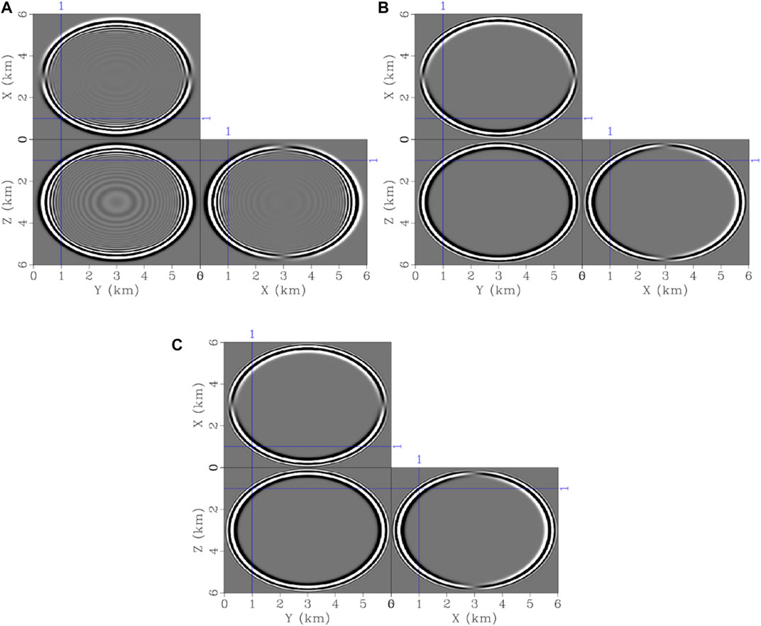
FIGURE 2. Wavefield snapshots $v_x$ obtained using the STS with the SGFD order of 2Nr = (A) 2, (B) 4 and (C) 6, at 0.96 s with a time step of 2.4-ms time marching.

FIGURE 3

FIGURE 3. Wavefield snapshots $v_x$ obtained using FTS with the SGFD (A) fourth- and (B) sixth-order spatial SGFD accuracy and using the STS with the SGFD (C) fourth- and (D) sixth-order spatial SGFD accuracy. The wavefield snapshots are recorded at 0.96 s with a time step of 2.4-ms time marching for the FTS method and 0.6-ms time marching for the STS method.

FIGURE 4

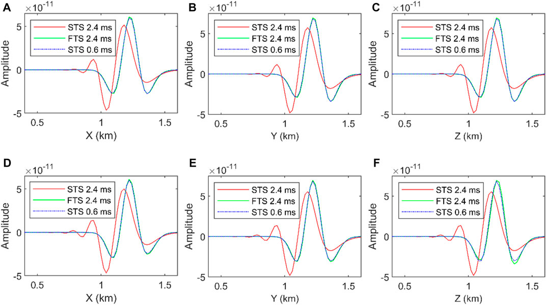
FIGURE 4. Profile comparisons at the positions of (A) and (D) (y, z) = (1, 1) km, (B) and (E) (x, z) = (1, 1) km, and (C) and (F) (x, y) = (1, 1) km. (A-C) are the results from the STS and FTS methods using the fourth-order accuracy in space, and (D-f) are the results from the STS and FTS methods using the sixth-order accuracy in space.

FIGURE 5

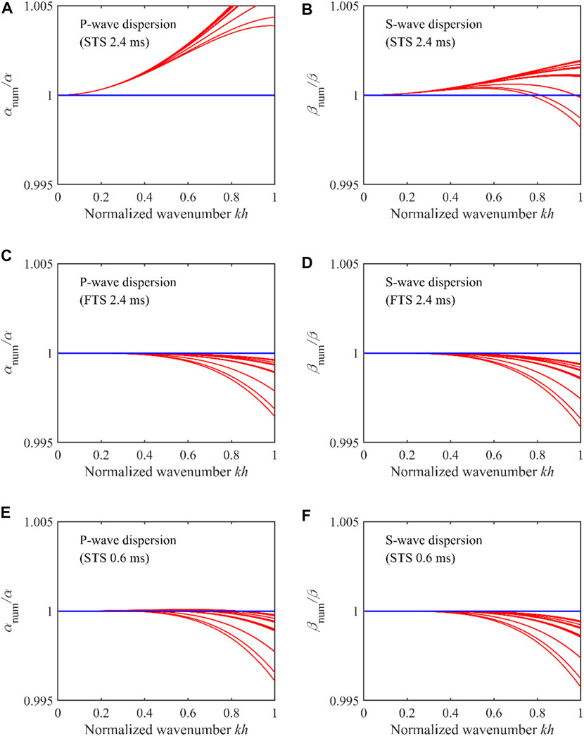
FIGURE 5. Dispersion curves for (A) and (B) the STS with a time step of 2.4 ms, (C) and (D) the FTS with a time step of 2.4 ms, and (E) and (F) the STS with a time step of 0.6 ms. (A), (C) and (E) are for P waves, and (B), (D) and (F) are for S waves. The fourth-order spatial SGFD accuracy is used. In each panel, they are twenty-five curves from bottom to top corresponding to the increases of two propagation angles of ${\theta }_1=0,\pi /16,...,\pi /4$ and ${\theta }_2=0,\pi /16,...,\pi /4$, respectively.

Spherical anomaly medium

The simulation accuracy of the temporal fourth-order accuracy method used in our proposed 3D ERTM is demonstrated in a spherical anomaly medium, as shown in Figure 6. Constant velocities of 3,600 and 1800 m/s are used for P and S waves in spherical anomaly, respectively, constant velocities of 3,000 and 2,160 m/s are used for P and S waves in the background, respectively, and the density is the constant of 2000 kg/m³. The model is discretized into 301 × 301 ×301 grid nodes with a spatial interval of 15 m, and the time step is 2.0 ms. The first derivative of the Gaussian function of 18 Hz is used as the explosive source located at the central point of the model.

FIGURE 6

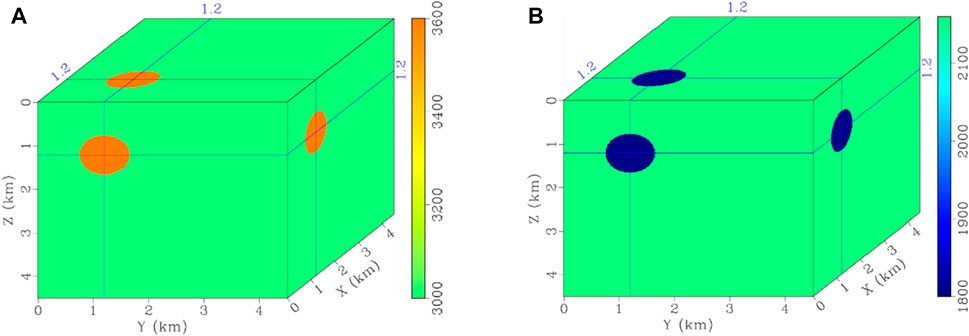
FIGURE 6. Spherical anomaly models of (A) and (B) true P- and S-wave velocity models.

In a spherical anomaly medium, both P and S waves can exist in wavefield snapshots, which can demonstrate that the scheme can properly optimize both P and S waves. The same spatial orders 2Nr =4 are used for the STS and FTS methods. Figure 7 displays the decupled P and S-wavefields of the STS and FTS methods. It is noted that the P wave and S wave are effectively separated based on vector-based decomposition for STS and FTS methods. The P- and S-wave profiles of both two methods are displayed in Figure 8 to make a further comparison. These profiles prove that the FTS method can obtain accurate P and S wavefields, with a good match with the reference results generated by the STS method using a 0.5-ms time step. One thing to be mentioned is that S waves also suffer from the temporal dispersion even in the explosive source because the P wavefield with errors is converted to S waves in the presence of impedance changes.

FIGURE 7

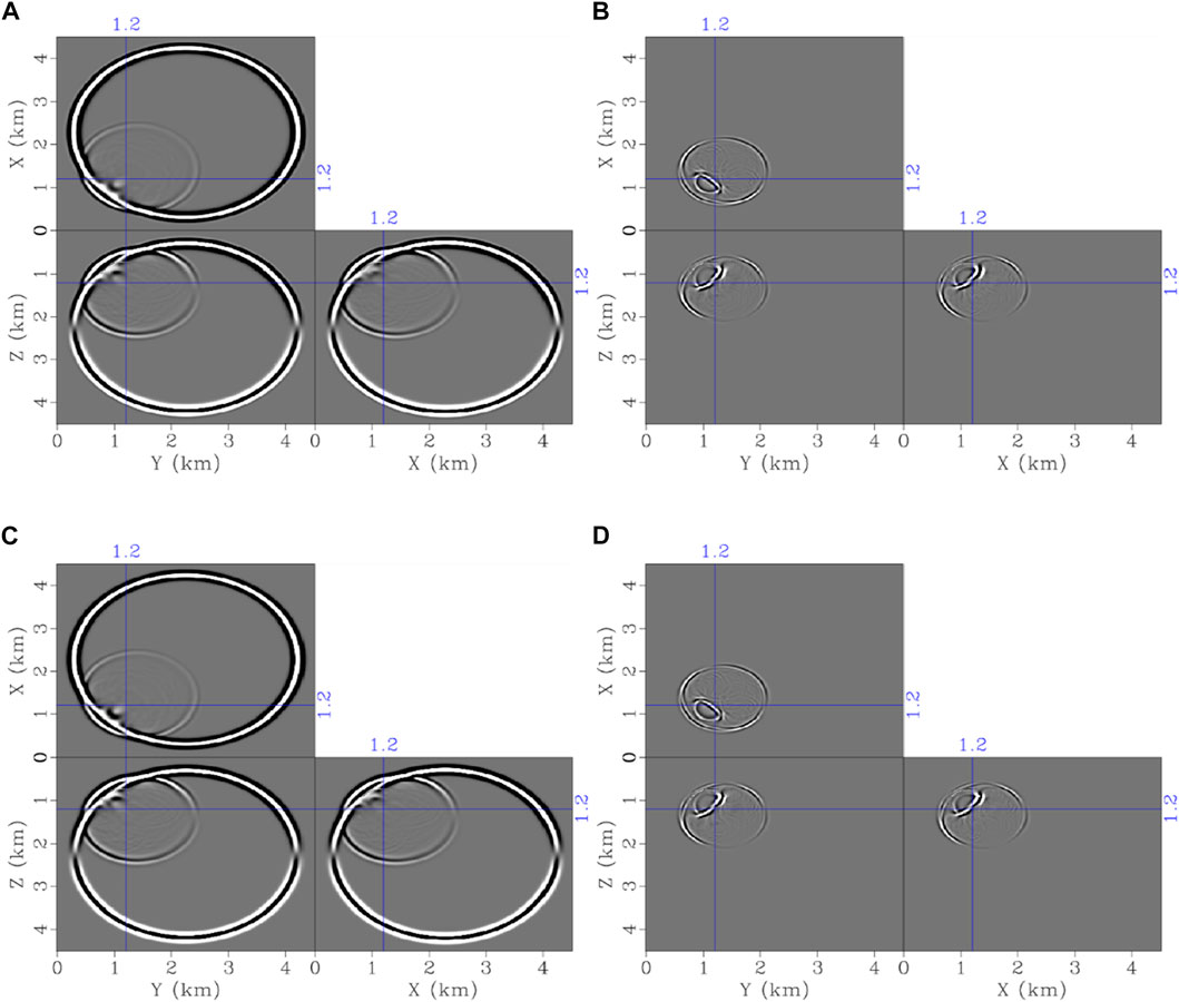
FIGURE 7. (A) and (B) P and S-wavefield snapshots $v_z$ obtained using the STS method, (C) and (D) P and S-wavefield snapshots $v_z$ obtained using the FTS method. The wavefield snapshots are recorded at 0.8 s with a time step of 2.0-ms time marching.

FIGURE 8

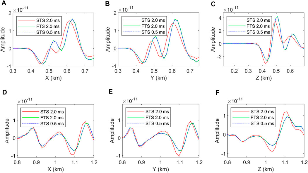
FIGURE 8. Profile comparisons at the positions of (A) and (D) (y, z) = (1.2, 1.2) km, (B) and (E) (x, z) = (1.2, 1.2) km, and (C) and (F) (x, y) = (1.2, 1.2) km. (A-C) are the P-wavefield results from the STS and FTS methods, and (D-F) are the S-wavefield results from the STS and FTS methods.

Efficiency analysis of wavefield simulation

The efficiency between the STS and FTS methods is also investigated here. Since the FTS method involves extra eight grid points in spatial partial derivative calculation, it introduces additional computational load. The SGFD was programmed using the GPU kernel, and the 3D models were mapped into a series of 3D GPU blocks. The GPU block size of 8 × 8 × 8 was chosen in the following efficiency tests. The time consumption of a 1-source/3000-time step simulation is tested for both methods in different SGFD orders and model sizes.

First, the simulation efficiency is tested in a homogeneous medium. The efficiency varying with SGFD orders is tested. The model size is 301 × 301 ×301 grid nodes. Figure 9A displays the time consumption varied with the SGFD orders for the STS and FTS methods. It was noted that the STS method was more efficient than the FTS method with the same time step in the order of 2Nr = 2, 4, and 8, whereas for the 2Nr = 6. The average time consumption of FTS is 1.41 times that of STS. As the accuracy comparisons above, the STS method using a three to four times smaller time step can nearly achieve antidispersion results, however, it requires at least two times the computation time of FTS. At the same time, we also tested the scalability of the algorithms of the two methods as the model size increased. Figure 9B shows that the two methods have better consistency in computing time, with an average time-consuming ratio of 1.37 for FTS to STS, when the model size increases.

FIGURE 9

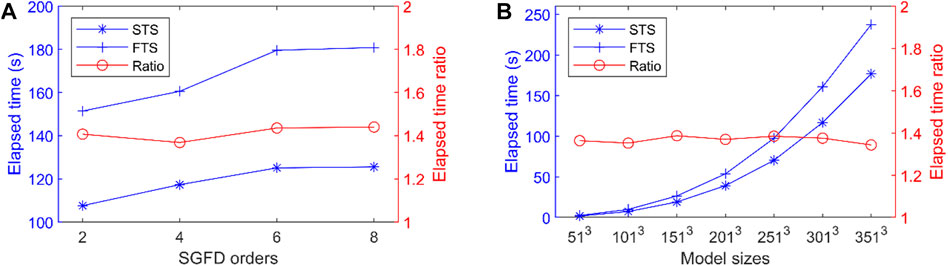
FIGURE 9. Efficiency comparisons of the STS and FTS method (A) with the increase of SGFD orders and (B) with the increase of model sizes. The model size is 301 × 301 ×301 in (A), and the fourth-order spatial accuracy is used in and (B). In (A) and (B), the left axis represents the time consumption and the right axis represents the time consumption ratio of FTS to STS.

Second, the simulation efficiency is tested in a linearly increasing velocity medium with a P-wave velocity range of 2000–6,000 m/s. The reason is that the velocity-dependent SGFD coefficients from a table for each spatial point at each time step may be expensive. The memory increase is negligible after using the rounding strategy, i.e., memory storage of an array of thousands of data points is small compared to the dozens of wavefield variables and model parameters over a million grid points. However, the frequent access of the SGFD coefficient at each spatial point at each time step is worth attention. The P-wave velocities are randomly generated in the velocity range, and S-wave velocities are transformed from P-wave velocities by assuming a Passion ratio of 1.732. There are 4001 SGFD coefficient pairs for the P wave and 2,354 pairs for the S wave by using the rounding strategy.

Figure 10A displays the time consumption of the STS and FTS methods as a function of the SGFD order in a model with 301 × 301 ×301 grid nodes as the SGFD order increases. Figure 10B shows the scalability of the algorithms of the two methods as the model size increases in the use of fourth-order spatial accuracy. The average time consumption of FTS is 1.52 and 1.47 times that of STS for Figures 10A,B, respectively. Compared to the FTS efficiency in the case of a homogeneous medium, heavy accesses to velocity-dependent SGFD coefficients can slightly increase the time consumption (∼7.47%) in the case of media with P- and S-wave velocity ranges of 2000–6,000 m/s and 1154.73–3,464.20, respectively. One thing to be mentioned is that only the SGFD computation part is used for timing without including the time for data recording and disk writing in the above efficiency tests.

FIGURE 10

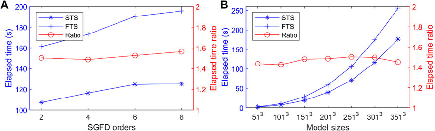
FIGURE 10. Efficiency comparisons of the STS and FTS method (A) with the increase of SGFD orders and (B) with the increase of model sizes. The model size is 301 × 301 ×301 in (A), and the fourth-order spatial accuracy is used in (B). In (A) and (B), the left axis represents the time consumption and the right axis represents the time consumption ratio of FTS to STS.

Modified SEG/EAGE overthrust model migration

The proposed method was first applied to a modified overthrust model of 2.2 km × 2.8 km × 2.8 km and sampled with a spatial interval of 20 m. Figures 11A,B display the true P- and S-wave velocities. A constant density of 2.0 g/cm³ was used, and the fourth-order spatial accuracy was used for all subsequent methods.

FIGURE 11

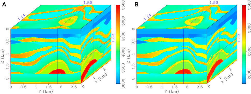
FIGURE 11. Modified overthrust models of (A) and (B) true P- and S-wave velocity models.

The wavefield decomposition of P and S waves is first shown in this section. The wavefield snapshots $v_z$ were displayed in Figure 12A, and its decoupled P- and S-wavefields were in Figures 12B,C, respectively. We noted that the decoupled wave equation form still performed well even for complex media because the short-wavelength S-wave and long-wavelength P-wave generated at the reflectors were separated from the aliased wavefield. In addition, it was worth noting that due to the explosive source used here, the S waves were mainly converted waves.

FIGURE 12

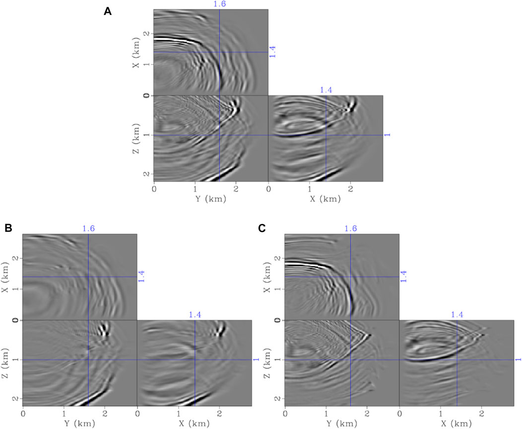
FIGURE 12. Wavefield snapshots $v_z$ of (A) full wavefield, (B) P-wavefield and (C) S-wavefield obtained using the FTS at the time of 0.96 s.

Before performing ERTM, we first observed the difference in synthetic data between the STS and FTS methods using the same 1.8-ms time step and 1.8-s record time. From the final comparisons in Figure 13, Figures 13A,B are similar. The trace comparisons in Figures 13C,D demonstrate the visible phase shift and waveform change compared with the reference generated using the STS method using a 0.45-ms time step. The visible phase shift manifests early arrivals of the reflective events. When comparing Figure 13 in more detail, we found the root-mean-square errors (RMSEs) of the normalized traces shown in Figure 13C were 0.2234 and 0.0750 for the STS and FTS methods, respectively. On an RTX 3090 GPU card, the 10-source/1.8-s simulation tests with the STS and FTS methods took 54.84 s and 74.68 s, respectively. Notably, a more accurate wavefield was obtained at the extra expense of a 36.18%-time cost.

FIGURE 13

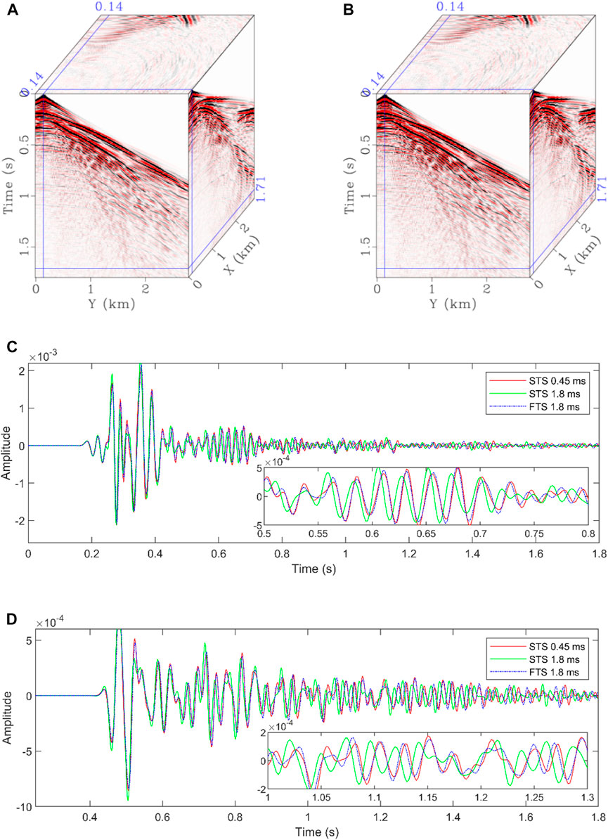
FIGURE 13. One-shot synthetic data v_z generated using the (A) STS and (B) FTS methods and seismic traces v_z comparisons between the results at (C) (x, y) = (1.0, 0.46) km and (D) (x, y) = (1.8, 0.46) km of the STS and the FTS methods with Δt = 1.8 ms and STS method with Δt = 0.45 ms.

Note that the time step of Δt = 1.8 ms is ∼99.12% of the allowed maximum time step of the STS method for this example. Because of the FTS method’s more relaxed CFL conditions, we set the time step to Δt = 2.1 ms, which is 99.41% of the allowed maximum P-wave time step (Fang et al., 2021). Then, the FTS method with a time step of Δt = 2.1 ms had an RMSE of 0.0853, and the 10-source/1.8-s simulation took 65.25 s. We concluded that relaxing the FTS method’s CFL conditions could reduce the extra calculation time from ∼36.18% to 18.98% but seldom reduce the accuracy (Figures 13C,D).

The ERTM improvement gained was investigated using an FTS simulation kernel. The migration velocities were obtained by smoothing the true velocities with a 3D window size of 160 × 160 × 160 m. A 25-Hz Ricker was used to generate the 225 shots as the observed data using the STS method with a fine time step of 0.45 ms. The total recorded time was 1.8 s. The direct waves for these observed data were removed in the ERTM, and two sets of ERTMs were performed using the STS and FTS schemes, respectively. The same 1.8-ms time step was shared for the two approaches. Figure 14 shows the final migration results. Although the two methods recovered the primary events, we still noticed the obvious imaging difference from the imaging slices as shown in Figure 15, especially for the zones indicated by the arrows. The imaging slices of the FTS method exhibit results consistent with the reference solution, whereas the STS method can produce certain artifacts.

FIGURE 14

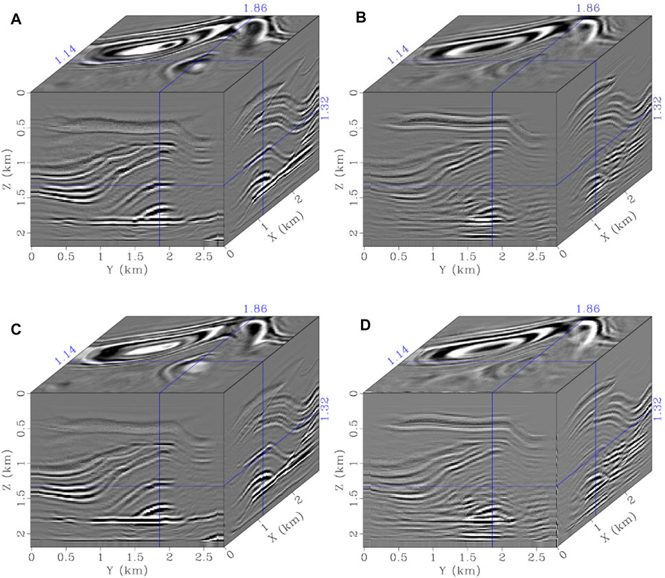
FIGURE 14. (A) and (B) PP and PS images using the STS method and (C) and (D) PP and PS images using the FTS method.

FIGURE 15

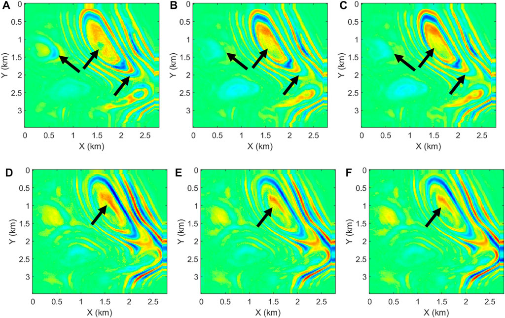
FIGURE 15. Image slices at z = 1.2 km using the (A) and (D) STS and (B) and (E) FTS methods and (C) and (F) references. (A), (B), and (C) are PP images, and (D), (E), and (F) are PS images.

Further, the profile comparisons shown in Figure 16 and Figure 17 demonstrate that when ERTM uses the STS modeling operator, the accuracy of images is reduced compared with the proposed ERTM using the FTS method. Specifically, for the PP images, the two horizontal profiles (Figures 16A,B) show the truth that the imaging positions of the conventional STS method become farther from the model’s center in the horizontal direction, whereas the vertical profile (Figure 16C) demonstrates the fact that the depth of the imaging horizon appears deep for the conventional STS method, with some degree of reflectance amplitude variation. For the PS images, although there is no obvious vertical deepening of imaging depth (Figure 17C), the imaging position shifts and amplitude changes in the horizontal position are obvious (Figures 17A,B). However, the proposed FTS method can overcome the above problems and obtain imaging results that match the reference solution very well for both PP and PS imaging, even with the same discrete time steps as used in the STS method.

FIGURE 16

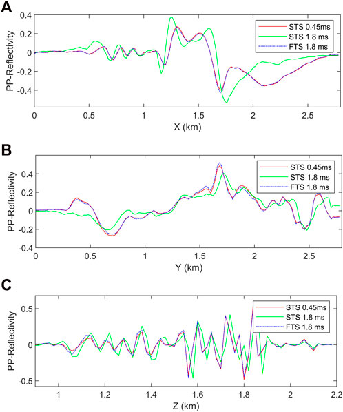
FIGURE 16. PP image profiles at (A) (y, z) = (1.6, 0.8) km, (B) (x, z) = (1.4, 1.8) km and (C) (x, y) = (2.0, 1.0) km via ERTMs using the STS and FTS methods.

FIGURE 17

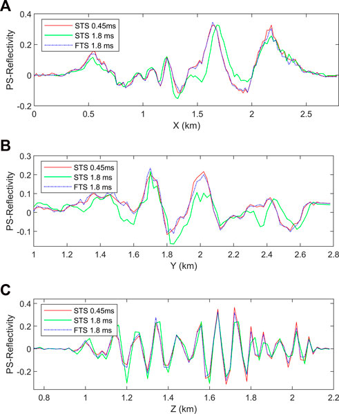
FIGURE 17. PS image profiles at (A) (y, z) = (1.6, 0.8) km, (B) (x, z) = (1.4, 1.8) km and (C) (x, y) = (2.0, 1.0) km via ERTMs using the STS and FTS methods.

At the same time, it is noted that there are larger imaging errors along horizontal directions than that along the vertical direction. One possible reason is that the surface geometry can record more reflections of vertical layers, thus providing better vertical stacking of images. By comparing Figure 16C and Figure 17C, it can be seen that the error of the PS image is smaller than that of the PP image. This is because the time dispersion of the P wave propagating at high velocities is more serious than that of the S wave propagating at low velocities, according to the dispersion analysis.

Modified salt model migration

The second ERTM example was evaluated on a modified salt model (Figure 18), with grid points of 150 × 150 × 100 in the x, y, and z directions and a grid size of 50 m. A constant density of 2.0 g/cm³ was used, and 150 shots were evenly distributed in the subsurface at a depth of 20 m. The first derivative of the Gaussian function with dominant frequency of 10 Hz was selected as the wavelet. These shots were generated as the observed data using the STS method with a fine time step of 1.0 ms.

FIGURE 18

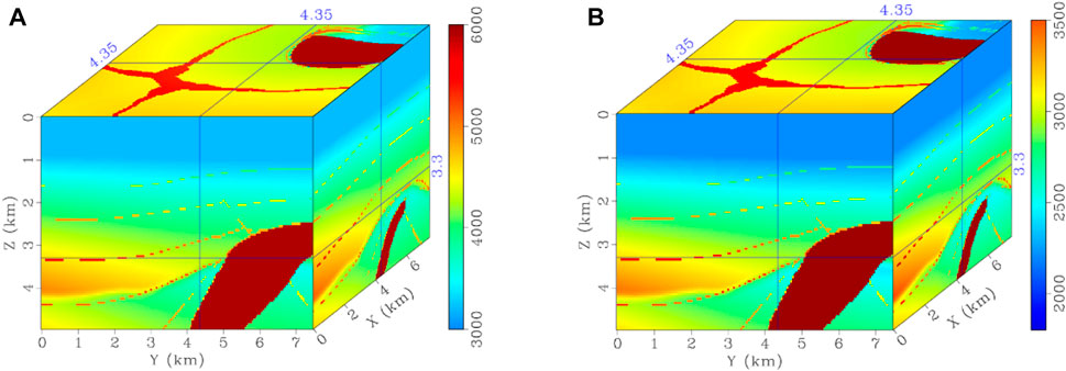
FIGURE 18. Modified salt models of (A) and (B) true P- and S-wave velocity models. Migration velocities are obtained by smoothing the true models using a 400 × 400 × 400 m smoother.

The migration velocities were obtained by smoothing the true velocities. We first generated the reference images by ERTM using the STS with a fine time step of 1.0 ms. Then, two sets of ERTMs were performed using the STS and FTS methods with the same 4.0-ms time step (Figures 19A–D). The slices at z = 4.5 km are displayed in Figure 20 to understand the images better. Figure 20 shows that the proposed ERTM using the FTS method successfully portrays the models’ accurate structures, and the images correlate with the reference images. However, the conventional ERTM using the STS method introduces some fakes due to the shift in the imaging location and the change in imaging amplitude caused by the temporal dispersion. Therefore, the PP and PS images in Figures 20B, E have more precise event boundaries than those in Figures 20A, D, especially for the areas indicated by the arrows. We also noticed some slight background noise in the imaging results, indicating the insufficient number of shots and smoothing of the background velocity models.

FIGURE 19

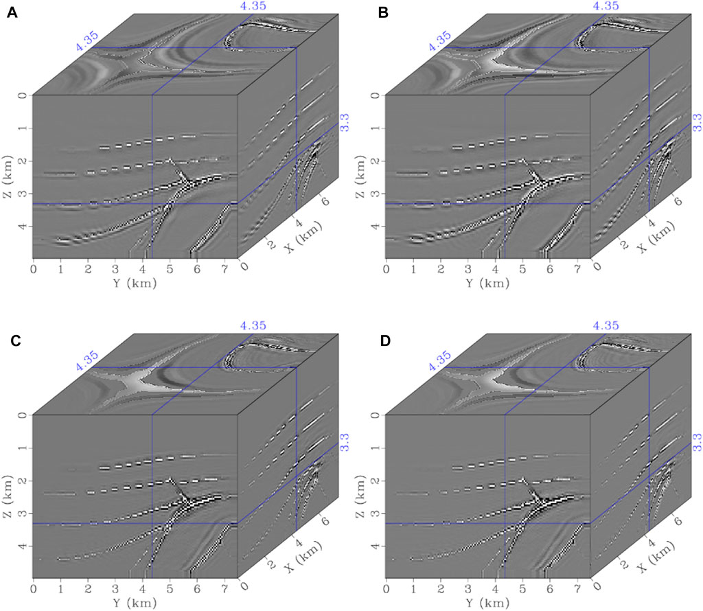
FIGURE 19. (A) and (B) PP and PS images using the STS method and (C) and (D) PP and PS images using the FTS method.

FIGURE 20

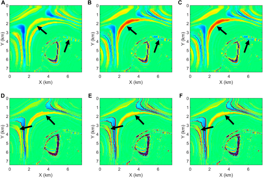
FIGURE 20. Image slices at z = 4.5 km using the (A) and (D) STS and (B) and (E) FTS methods and (C) and (F) references. (A), (B), and (C) are PP images, and (D), (E), and (F) are PS images.

The above simulation and two image results show that the proposed 3D ERTM using an FTS method achieves high-accuracy migration, especially when using a large time step. The errors caused by second-order temporal accuracy deepen and extend the imaging locations vertically and horizontally, respectively. Furthermore, the images might become distorted in deep areas when ERTM uses the STS method.

Discussion

In high-accuracy imaging, we only considered the fourth-order temporal accuracy because Chen et al. (2016b) had demonstrated slight accuracy improvement from the fourth-order to the sixth-order. Therefore, the fourth-order temporal accuracy is sufficient for high-precision RTM imaging without incurring much additional computational cost (Tan and Huang, 2014). The SGFD coefficient calculation includes velocity parameters and precalculating velocity-dependent SGFD coefficients before the differential calculation can improve efficiency. Meanwhile, velocity rounding is a good choice that avoids more pairs of coefficients.

Other ERTM or least-square ERTM techniques (Duan et al., 2017; Feng and Schuster, 2017; Xu et al., 2021; Song et al., 2022.) can be introduced or developed based on the proposed ERTM workflow to suppress the numerical temporal and spatial dispersion. In addition, in anisotropic media, the SGFD coefficients and the wavefield decomposition related to the model parameters should be carefully considered and rederived.

Conclusion

This study develops a high-accuracy 3D ERTM using a temporal fourth-order and arbitrary spatial even-order SGFD simulation kernel. The ERTM workflow uses an advanced 3D P- and S-wave decoupled quasi-stress–velocity wave equation and source-energy-normalized vector-based elastic imaging conditions. The proposed method effectively suppresses the temporal dispersion in traditional second-order temporal accuracy SGFD schemes, ensuring accurate image locations from a numerical simulation perspective. The proposed method using the velocity-independent SGFD coefficients takes more time, but employing a large time step can effectively reduce the time consumption in a certain process. The highlighted numerical examples demonstrate that the proposed 3D ERTM achieves precise and reliable images. The proposed high-accuracy 3D ERTM workflow helps to integrate the most advanced imaging techniques into this computational framework.

Data availability statement

The original contributions presented in the study are included in the article/Supplementary Material, further inquiries can be directed to the corresponding author.

Author contributions

JF: Methodology, Formal analysis, Visualization, Writing—Original Draft LH: Investigation, Visualization, Validation YS: Supervision, Conceptualization, Writing—Review and Editing HC: Software, Writing—Review and Editing BW: Formal analysis, Writing—Review and Editing.

Funding

This work is supported in part by the National Key R&D Program of China (2022YFC3003300), National Natural Science Foundation of China (42104113, 41930431), and Natural Science Foundation of Jiangsu Province of China (BK20210526).

Conflict of interest

The authors declare that the research was conducted in the absence of any commercial or financial relationships that could be construed as a potential conflict of interest.

Publisher’s note

All claims expressed in this article are solely those of the authors and do not necessarily represent those of their affiliated organizations, or those of the publisher, the editors and the reviewers. Any product that may be evaluated in this article, or claim that may be made by its manufacturer, is not guaranteed or endorsed by the publisher.

References

Alkhalifah, T. (2013). Residual extrapolation operators for efficient wavefield construction. Geophys J. Int. 193 (2), 1027–1034. doi:10.1093/gji/ggt040

CrossRef Full Text | Google Scholar

Bleistein, N. (1987). On the imaging of reflectors in the Earth. Geophysics 52 (7), 931–942. doi:10.1190/1.1442363

CrossRef Full Text | Google Scholar

Chang, W. F., and McMechan, G. A. (1987). Elastic reverse-time migration. Geophysics 52 (10), 1365–1375. doi:10.1190/1.1442249

CrossRef Full Text | Google Scholar

Chen, H., Zhou, H., and Sheng, S. (2016a). General rectangular grid-based time-space domain high-order finite-difference methods for modeling scalar wave propagation. J. Appl. Geophys. 133, 141–156. doi:10.1016/j.jappgeo.2016.07.021

CrossRef Full Text | Google Scholar

Chen, H., Zhou, H., Zhang, Q., and Chen, Y. (2016b). Modeling elastic wave propagation using K-space operator-based temporal high-order staggered-grid finite-difference method. IEEE Trans. Geosci. Remote Sens. 55 (2), 801–815. doi:10.1109/TGRS.2016.2615330

CrossRef Full Text | Google Scholar

Chen, J. B. (2007). High-order time discretizations in seismic modeling. Geophysics 72 (5), SM115–SM122. doi:10.1190/1.2750424

CrossRef Full Text | Google Scholar

Claerbout, J. F., and Doherty, S. M. (1972). Downward continuation of moveout-corrected seismograms. Geophysics 37 (5), 741–768. doi:10.1190/1.1440298

CrossRef Full Text | Google Scholar

Courant, R., Friedrichs, K., and Lewy, H. (1928). Über die partiellen Differenzengleichungen der mathematischen Physik. Math. Ann. 100 (1), 32–74. doi:10.1007/BF01448839

CrossRef Full Text | Google Scholar

Du, Q., Gong, X., Zhang, M., Zhu, Y., and Fang, G. (2014a). 3D PS-wave imaging with elastic reverse-time migration. Geophysics 79 (5), S173–S184. doi:10.1190/geo2013-0253.1

CrossRef Full Text | Google Scholar

Du, X., Fowler, P., J., and Fletcher, R. P. (2014b). Recursive integral time-extrapolation methods for waves: A comparative review. Geophysics 79 (1), T9–T26. doi:10.1190/geo2013-0115.1

CrossRef Full Text | Google Scholar

Du, Q., Guo, C., Zhao, Q., Gong, X., Wang, C., and Li, X. Y. (2017). Vector-based elastic reverse time migration based on scalar imaging condition. Geophysics 82 (2), S111–S127. doi:10.1190/geo2016-0146.1

CrossRef Full Text | Google Scholar

Duan, Y., Guitton, A., and Sava, P. (2017). Elastic least-squares reverse time migration. Geophysics 82 (4), S315–S325. doi:10.1190/geo2016-0564.1

CrossRef Full Text | Google Scholar

Etgen, J. T., and Brandsberg-Dahl, S. (2009). “The pseudo-analytical method: Application of pseudo-Laplacians to acoustic and acoustic anisotropic wave propagation,” in Society of Exploration Geophysicists SEG Technical Program Expanded Abstracts 2009 (Houston, TX: Society of Exploration Geophysicists), 2252–2256.

Google Scholar

Fang, G., Fomel, S., Du, Q., and Hu, J. (2014). Lowrank seismic-wave extrapolation on a staggered grid. Geophysics 79 (3), T157–T168. doi:10.1190/geo2013-0290.1

CrossRef Full Text | Google Scholar

Fang, J., Chen, H., Zhou, H., Rao, Y., Sun, P., and Zhang, J. (2020). Elastic full-waveform inversion based on GPU accelerated temporal fourth-order finite-difference approximation. Comput. Geosci. 135, 104381. doi:10.1016/j.cageo.2019.104381

CrossRef Full Text | Google Scholar

Fang, J., Chen, H., Zhou, H., Zhang, Q., and Wang, L. (2021). Three-dimensional elastic full-waveform inversion using temporal fourth-order finite-difference approximation. IEEE Geosci. Remote. Sens. Lett. 19, 1–5. doi:10.1109/LGRS.2021.3125310

CrossRef Full Text | Google Scholar

Fang, J., Shi, Y., Zhou, H., Chen, H., Zhang, Q., and Wang, N. (2022a). A high-precision elastic reverse-time migration for complex geologic structure imaging in applied Geophysics. Remote Sens. 14 (15), 3542. doi:10.3390/rs14153542

CrossRef Full Text | Google Scholar

Fang, J., Zhou, H., Zhang, J., Zhang, Q., Liu, S., and Wang, B. (2022b). 3D elastic multisource full waveform inversion on distributed GPU clusters. J. Appl. Geophys. 199, 104595. doi:10.1016/j.jappgeo.2022.104595

CrossRef Full Text | Google Scholar

Feng, Z., and Schuster, G. T. (2017). Elastic least-squares reverse time migration. Geophysics 82 (2), S143–S157. doi:10.1190/geo2016-0254.1

CrossRef Full Text | Google Scholar

Fomel, S., Ying, L., and Song, X. (2013). Seismic wave extrapolation using lowrank symbol approximation. Geophys. Prospect. 61 (3), 526–536. doi:10.1111/j.1365-2478.2012.01064.x

CrossRef Full Text | Google Scholar

Gazdag, J. (1978). Wave equation migration with the phase-shift method. Geophysics 43 (7), 1342–1351. doi:10.1190/1.1440899

CrossRef Full Text | Google Scholar

Koene, E. F., Robertsson, J. O., Broggini, F., and Andersson, F. (2018). Eliminating time dispersion from seismic wave modeling. Geophys. J. Int. 213 (1), 169–180. doi:10.1093/gji/ggx563

CrossRef Full Text | Google Scholar

Kosloff, D., Filh, A. Q., Tessmer, E., and Behle, A. (1989). Numerical solution of the acoustic and elastic wave equations by a new rapid expansion method. Geophys Prospect 37 (4), 383–394. doi:10.1111/j.1365-2478.1989.tb02212.x

CrossRef Full Text | Google Scholar

Kristek, J., Moczo, P., and Galis, M. (2010). Stable discontinuous staggered grid in the finite-difference modelling of seismic motion. Geophys. J. Int. 183 (3), 1401–1407. doi:10.1111/j.1365-246X.2010.04775.x

CrossRef Full Text | Google Scholar

Li, H., and Li, J. (2022). Elastic transmitted wave reverse time migration for imaging earth’s interior discontinuities: A numerical study. Bull. Seismol. Soc. Am. 112, 2231–2256. doi:10.1785/0120210325

CrossRef Full Text | Google Scholar

Li, Y. E., Wong, M., and Clapp, R. (2016). Equivalent accuracy at a fraction of the cost: Overcoming temporal dispersion. Geophysics 81 (5), T189–T196. doi:10.1190/geo2015-0398.1

CrossRef Full Text | Google Scholar

McMechan, G. A. (1983). Migration by extrapolation of time-dependent boundary values. Geophys Prospect 31 (3), 413–420. doi:10.1111/j.1365-2478.1983.tb01060.x

CrossRef Full Text | Google Scholar

Pestana, R. C., and Stoffa, P. L. (2010). Time evolution of the wave equation using rapid expansion method. Geophysics 75 (4), T121–T131. doi:10.1190/1.3449091

CrossRef Full Text | Google Scholar

Ren, Z., and Li, Z. (2019). High-order temporal and implicit spatial staggered-grid finite-difference operators for modelling seismic wave propagation. Geophys. J. Int. 217 (2), 844–865. doi:10.1093/gji/ggz059

CrossRef Full Text | Google Scholar

Ren, Z., Li, Z., Liu, Y., and Sen, M. K. (2017). Modeling of the acoustic wave equation by staggered-grid finite-difference schemes with high-order temporal and spatial accuracy. Bull. Seismol. Soc. Am. 107 (5), 2160–2182. doi:10.1785/0120170068

CrossRef Full Text | Google Scholar

Ren, Z., Bao, Q., and Gu, B. (2021). Time-dispersion correction for arbitrary even-order Lax-Wendroff methods and the application on full-waveform inversion. Geophysics 86 (5), T361–T375. doi:10.1190/geo2020-0934.1

CrossRef Full Text | Google Scholar

Shi, Y., Zhang, W., and Wang, Y. (2019). Seismic elastic RTM with vector-wavefield decomposition. J. Geophys. Eng. 16 (3), 509–524. doi:10.1093/jge/gxz023

CrossRef Full Text | Google Scholar

Song, X., Fomel, S., and Ying, L. (2013). Lowrank finite-differences and lowrank Fourier finite-differences for seismic wave extrapolation in the acoustic approximation. Geophys. J. Int. 193 (2), 960–969. doi:10.1093/gji/ggt017

CrossRef Full Text | Google Scholar

Song, L., Shi, Y., Liu, W., and Zhao, Q. (2022). Elastic reverse time migration for weakly illuminated structure. App. Sci. 12 (10), 5264. doi:10.3390/app12105264

CrossRef Full Text | Google Scholar

Stewart, R. R., Gaiser, J. E., Brown, R. J., and Lawton, D. C. (2003). Converted-wave seismic exploration: Applications. Geophysics 68 (1), 40–57. doi:10.1190/1.1543193

CrossRef Full Text | Google Scholar

Tan, S., and Huang, L. (2014). An efficient finite-difference method with high-order accuracy in both time and space domains for modelling scalar-wave propagation. Geophys.J. Int. 197 (2), 1250–1267. doi:10.1093/gji/ggu077

CrossRef Full Text | Google Scholar

Tessmer, E. (2011). Using the rapid expansion method for accurate time-stepping in modeling and reverse-time migration. Geophysics 76 (4), S177–S185. doi:10.1190/1.3587217

CrossRef Full Text | Google Scholar

Virieux, J. (1986). P-SV wave propagation in heterogeneous media: Velocity-stress finite-difference method. Geophysics 51 (4), 889–901. doi:10.1190/1.1442147

CrossRef Full Text | Google Scholar

Wang, M., and Xu, S. (2015). Finite-difference time dispersion transforms for wave propagation. Geophysics 80 (6), WD19–WD25. doi:10.1190/geo2015-0059.1

CrossRef Full Text | Google Scholar

Wang, C., Cheng, J., and Arntsen, B. (2016). Scalar and vector imaging based on wave mode decoupling for elastic reverse time migration in isotropic and transversely isotropic media. Geophysics 81 (5), S383–S398. doi:10.1190/geo2015-0704.1

CrossRef Full Text | Google Scholar

Wang, W., Hua, B., McMechan, G. A., and Duquet, B. (2018). P-and S-decomposition in anisotropic media with localized low-rank approximations. Geophysics 83 (1), C13–C26. doi:10.1190/geo2017-0138.1

CrossRef Full Text | Google Scholar

Whitmore, N. D. (1983). “Iterative depth migration by backward time propagation,” in SEG Technical Program expanded abstracts 1983 (Las Vegas, NV: Society of Exploration Geophysicists), 382–385. doi:10.1190/1.1893867

CrossRef Full Text | Google Scholar

Wu, B., Tan, W., Xu, W., and Li, B. (2022). Trapezoid-grid finite difference time domain method for 3D seismic wavefield modeling using CPML absorbing boundary condition. Front. Earth Sci. 9, 1297. doi:10.3389/feart.2021.777200

CrossRef Full Text | Google Scholar

Wu, Z., and Alkhalifah, T. (2014). The optimized expansion based low-rank method for wavefield extrapolation. Geophysics 79 (2), T51–T60. doi:10.1190/geo2013-0174.1

CrossRef Full Text | Google Scholar

Xu, S., Liu, Y., Ren, Z., and Zhou, H. (2019). Time-space-domain temporal high-order staggered-grid finite-difference schemes by combining orthogonality and pyramid stencils for 3D elastic-wave propagation. Geophysics 84 (4), T259–T282. doi:10.1190/geo2018-0551.1

CrossRef Full Text | Google Scholar

Xu, H., Wang, X., Wang, C., and Zhang, J. (2021). Sparse constrained least-squares reverse time migration based on Kirchhoff approximation. Front. Earth Sci. 9, 770. doi:10.3389/feart.2021.731697

CrossRef Full Text | Google Scholar

Yan, J., and Sava, P. (2008). Isotropic angle-domain elastic reverse-time migration. Geophysics 73 (6), S229–S239. doi:10.1190/1.2981241

CrossRef Full Text | Google Scholar

Yang, J., Zhu, H., Huang, J., and Li, Z. (2018a). 2D isotropic elastic Gaussian-beam migration for common-shot multicomponent records. Geophysics 83 (2), S127–S140. doi:10.1190/geo2017-0078.1

CrossRef Full Text | Google Scholar

Yang, J., Zhu, H., Wang, W., Zhao, Y., and Zhang, H. (2018b). Isotropic elastic reverse time migration using the phase-and amplitude-corrected vector P-and S-wavefields. Geophysics 83 (6), S489–S503. doi:10.1190/geo2018-0023.1

CrossRef Full Text | Google Scholar

Yong, P., Huang, J., Li, Z., Liao, W., Qu, L., Li, Q., et al. (2016). Elastic-wave reverse-time migration based on decoupled elastic-wave equations and inner-product imaging condition. J. Geophys. Eng. 13 (6), 953–963. doi:10.1088/1742-2132/13/6/953

CrossRef Full Text | Google Scholar

Zhang, Q., and McMechan, G. A. (2010). 2D and 3D elastic wavefield vector decomposition in the wavenumber domain for VTI media. Geophysics 75 (3), D13–D26. doi:10.1190/1.3431045

CrossRef Full Text | Google Scholar

Zhang, R., Huang, J. P., Zhuang, S. B., and Li, Z. C. (2019). Target-oriented Gaussian beam migration using a modified ray tracing scheme. Pet. Sci. 16 (6), 1301–1319. doi:10.1007/s12182-019-00388-y

CrossRef Full Text | Google Scholar

Zhou, H., Liu, Y., and Wang, J. (2021a). Acoustic finite-difference modeling beyond conventional Courant-Friedrichs-Lewy stability limit: Approach based on variable-length temporal and spatial operators. Earthq. Sci. 34 (2), 123–136. doi:10.29382/eqs-2021-0009

CrossRef Full Text | Google Scholar

Zhou, H., Liu, Y., and Wang, J. (2021b). Elastic wave modeling with high-order temporal and spatial accuracies by a selectively modified and linearly optimized staggered-grid finite-difference scheme. IEEE Trans. Geosci. Remote Sens. 60. doi:10.1109/TGRS.2021.3078626

CrossRef Full Text | Google Scholar

Zhu, H. (2017). Elastic wavefield separation based on the Helmholtz decomposition. Geophysics 82 (2), S173–S183. doi:10.1190/geo2016-0419.1

CrossRef Full Text | Google Scholar