Machine learning based ground motion site amplification prediction

Site condition impact on seismic ground motion has been a complex but important subject in earthquake hazard analysis. Traditional studies on site amplification effect are either based on site response via wave propagation simulation or regression analysis using parameters such as Vs30, bedrock ground motion and site response period. Ground Motion Prediction Equations (GMPEs) are used for regions where there is limited data of seismic records. The main issues with these approaches are that they cannot demonstrate the complex relationship between site amplification and its various affecting parameters, thus there exists large uncertainty in the results. Recent studies based on machine learning have shown significant improvement in predicting the site amplification, but the result is not well explained. This study assembled the information on 6 parameters including Vs30, magnitude, epicentral distance, earthquake source depth, bedrock ground motion, and altitude of 353,327 records observed during 1997 and 2019 from 698 KiK-net stations. Three machine learning algorithms of Random Forest (RF), XGBoost, and Deep Neural Networks (DNN) were implemented to predict the site amplification factor using these 6 selected parameters. Shapley Additive explanation (SHAP) was used to explain the importance of the 6 parameters. The results show that all three machine learning algorithms performed much better than the traditional GMPE approach with XGBoost’s performance the best. The explanation provided by the SHAP analysis further enhanced the reasonability of this study. It is anticipated that the combination of machine learning and SHAP analysis can provide better assessment for site amplification of ground motion with better potential of future application in seismic hazard analysis.

1 Introduction

The effect of site condition on seismic ground motion has been a research focus in geotechnical earthquake engineering and seismic hazard analysis. Numerous records have demonstrated that site conditions amplify the ground motion and further intensify the earthquake damage (Borcherdt, 1970; Borcherdt and Gibbs, 1976; Seed et al., 1988; Dobry et al., 2000; Bala et al., 2009). A large number of studies have been performed to better represent the effect of site amplification, and traditional approaches can be categorized into two groups: site response analysis based on wave propagation simulation and the empirical Ground Motion Prediction Equations (GMPEs). Site response analysis based on site wave propagation simulation is mostly using one-dimensional (1-D) or multi-dimensional models. The non-linear property of the soil is approximated through equivalent linearization (Idriss and Seed, 1968; Seed and Idriss, 1969). Park and Hashash conducted the analysis through improved equivalent linearization of site soil non-linear property (Park and Hashash, 2004; Park and Hashash, 2008), and Gerlymos and Gazetas proposed a new constitutive model in a 1-D analysis (Gerolymos and Gazetas, 2005). Harmon et al. developed the ground motion site amplification model for the West and East part of the US based on extensive site response simulation (Harmon et al., 2019). Site response analysis can provide detailed results of the site amplification, but the analysis requires extensive information on soil property which is often not available. The other approach for site response analysis is through empirical Ground Motion Prediction Equations (GMPEs), which is a statistical model based on earthquake property and simplified parameters of site soil conditions. The early stage GMPEs were usually developed separately for rock and soil site conditions, and ground motion amplification factor was used to consider statistical effect of site conditions (Boore et al., 1997; Sadigh et al., 1997). Abrahamson and Silva considered non-linear effect of the site amplification factor (Abrahamson and Silva, 1997), and Boore et al. (Boore et al., 1997) used the average shear-wave velocity of the top 30 m soils (Vs30) to represent the site effect. Seyhan and Stewart (Seyhan and Stewart, 2014) developed a site amplification model for the West part of the US and used the GMPEs by Boore et al. (Boore et al., 2014) for rock sites to compliment the data scarcity of records on rock sites. Most GMPEs used only Vs30 to express the site condition, which cannot completely represent the complex nature of the various site conditions, thus resulting in a large degree of uncertainty. With the accumulation of a great number of observed records and rapid development of computational resources machine learning algorithms have been actively introduced to predict the site response. Daniel Roten et al. (Roten and Olsen, 2021a) applied machine learning to predict the site amplification factor using records from the KiK-net, and the result was compared against the result by the 1-D site response analysis showing the mean squared logarithm error reduction of at least 50%. Hamidreza et al. (Hamidreza and Soleimani Kutanaei, 2015) compared the site amplification result by Artificial Neural Network (ANN) against the result by 2-D site response analysis and found that the shear wave velocity and soil layer depth are more important than other factors in site amplification. Kveh (Kaveh et al., 2016)and (Derras et al., 2017) predicted the site amplification through M5 decision tree method and ANN, respectively. Chuanbin Zhu (Zhu et al., 2021)compared the performance of RF, GRA, SRI and HVSR methods on the benchmark dataset, and the results showed that RF performance is relatively better. Daniel Roten (Roten and Olsen, 2021b) compared the neural network methods (CNN, MLP) with the theoretical SH1D amplification method, and the results showed that CNN has a smaller MSLE and MAE in the prediction results. Machine learning approach has shown its superiority in predicting site amplification of ground motion, but the approach itself looked like a “black box” approach with results somethings difficult to be explained.

This study utilized the observed ground motion in KiK-net between 1997 and 2019, and applied RF, XGBoost, and DNN approaches to predict site amplification factor for different periods. The results were compared against those by (Yoojoong and Jonathan, 2005), who used Vs30 as the main parameter to predict ground motion site amplification. The comparison demonstrates that machine learning approaches are superior in predicting site amplification with XGBoost performance the best. Shapley additive explanation (SHAP) was then introduced to explain the proposed prediction models, and the contribution of each parameter on site amplification was analyzed to provide better guidance for future similar studies.

2 Data

KiK-net is the ground motion observation network operated by the Japanese National Research Institute for Earth Science and Disaster Resilience (NIED), which is composed of approximately 700 stations (https://www.doi.org/10.17598/NIED.0004). Each station has a pair of high-end sensors placed at the top and bottom of the borehole to record three components (NS, EW, UD) of the earthquake ground motion. In addition, detailed soil profile data has been provided for most stations by NIED. This study conducted the research based the data accumulated by KiK-net during 1997–2019.

2.1 Data preparation

The ground motion records by KiK-net are stored separately for each earthquake event, and this study assembled the records with the following additional parameters. Information on earthquake magnitude (Mag), altitude of the station (S_Altitude), earthquake source depth (Depth), and the latitude and longitude of both the earthquake source and the observation stations are included in the ground motion records. The epicentral distance(R) can be calculated via the latitude and longitude of the earthquake source and observation stations. The Vs30 at the stations can be calculated from the borehole data according to Eq. 1 (Yoojoong and Jonathan, 2005). For stations where borehole data does not reach down to 30 m, the last layer will be extended to 30 m deep (Boore, 2004).

${\mathit{V}}_{\mathbf{30}}=\mathbf{30}/{\displaystyle \sum }_{\mathbf{1}}^{\mathit{n}}\frac{{\mathit{d}}_{\mathit{i}}}{{\mathit{V}\mathit{s}}_{\mathit{i}}}(1)$

where ${\mathit{d}}_{\mathit{i}}$ is the depth for the $\mathit{i}$-th layer, and ${\mathit{V}\mathit{s}}_{\mathit{i}}$ is its corresponding shear wave velocity. The calculation only accounts for soil layers up to 30 m deep. Spectral acceleration Sa is calculated as in Eq. 2 (Chen Longwei Chen Zhuoshi Yuan Xiaoming, 2013).

$\mathit{S}\mathit{a}\left(\mathit{T}\right)=\sqrt{{\mathit{S}\mathit{a}\left(\mathit{T}\right)}_{\mathit{E}\mathit{W}}\ast {\mathit{S}\mathit{a}\left(\mathit{T}\right)}_{\mathit{N}\mathit{S}}}(2)$

where ${\mathit{S}\mathit{a}\left(\mathit{T}\right)}_{\mathit{E}\mathit{W}}$, ${\mathit{S}\mathit{a}\left(\mathit{T}\right)}_{\mathit{N}\mathit{S}}$ are the spectral acceleration of the $\mathit{E}\mathit{W}$ and $\mathit{N}\mathit{S}$ component for period $\mathit{T}$.

The site amplification factor ($\mathrm{A}\mathrm{m}\mathrm{p}$) for Sa can be calculated as in Eq. 3.

$\mathit{A}\mathit{m}\mathit{p}\left(\mathit{T}\right)=\frac{{\mathit{S}\mathit{a}\left(\mathit{T}\right)}_{\mathit{S}}}{{\mathit{S}\mathit{a}\left(\mathit{T}\right)}_{\mathit{R}}}(3)$

where ${\mathit{S}\mathit{a}\left(\mathit{T}\right)}_{\mathit{S}}$, ${\mathit{S}\mathit{a}\left(\mathit{T}\right)}_{\mathit{R}}$ are the SA at surface and bottom respectively for period $\mathit{T}$. The above computation is repeated for all the records observed in the KiK-net during 1997–2019, resulting in a data set of Amp for more than 350,000 earthquake records.

2.2 Data filtering and distribution

The location distribution of earthquake source and observation station for the dataset selected in this study is shown in Figure 1. Previous researches (Bommer and Martinez-Pereira, 2000) have shown that only ground motions with PGA more than 20 cm/s² will have impact on our society, engineering structures and living environment. The PGA_S (subscript s stands for surface) distribution of the data collected for this study is shown in Figure 2A, and from Figure 2A it can be seen that PGA_S for most records is below 20 cm/s². For application in future engineering practice, we need to filter the data from the assembled dataset. Figure 2B shows the distribution of Amp with datasets of different minimum PGA_S of 0, 1, 2, and 20 cm/s². As can be seen from Figure 2B, the distribution of Amp for datasets of minimum 1 cm/s² and 20 cm/s² looks similar, therefore, we chose the dataset with minimum PGA_S of 1 cm/s² for this study to ensure that there be enough samples in the dataset. This filtered dataset has more than 260,000 samples. The distribution of Vs30, Mag, R and Depth for the selected dataset is also shown in Figures 3A–D, respectively. As can be seen from Figure 3 Vs30 mostly falls into the range of 250–700 m/s, and M is mostly between 4 and 7, while R is mostly less than 200 km and the source depth is mostly shallower than 60 km.

FIGURE 1

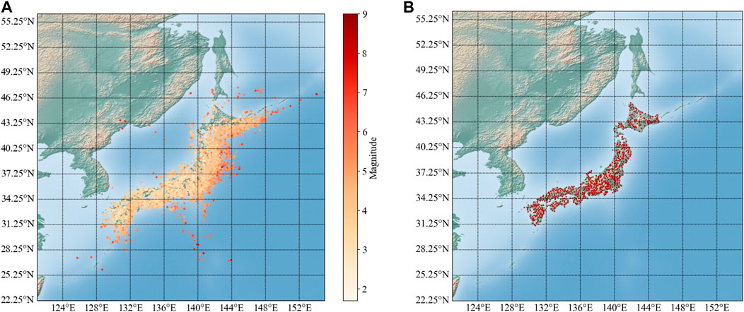
FIGURE 1. Location distribution of earthquake source and observation station. (A) Earthquake source location, (B) Observation station location.

FIGURE 2

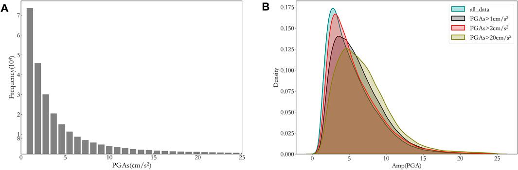
FIGURE 2. Record frequency distribution with PGAs or its amplification. (A) PGAs distribution for all records, (B) Amp (PGA) distribution of datasets with different filtrating PGA_S.

FIGURE 3

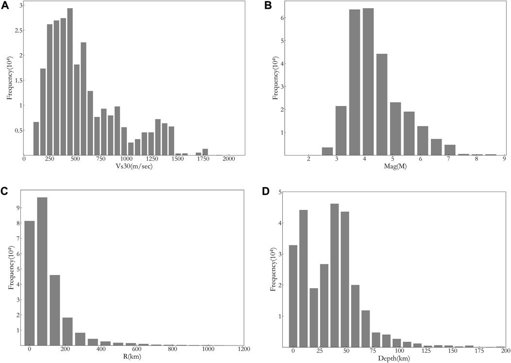
FIGURE 3. Distribution of the dataset for different parameters. (A) Vs30, (B) Magnitude, (C) Epicentral distance and (D) Source depth.

3 Models for predicting

3.1 Traditional approach

Most traditional approaches use parameters such as Vs30 and PGA_R to predict the site amplification factor. (Yoojoong and Jonathan, 2005) established a site amplification prediction equation using Vs30 and PGA_R and verified its effectiveness via comparison with actual amplification based on a large number of ground motion records. Their results also demonstrated explicit deviation from the NEHRP provision of amplification factors. Their prediction formula can be shown in Eq. 4.

$\mathit{Ln}\left(\mathit{A}\mathit{m}\mathit{p}\right)=\mathbf{c}\mathbf{ln}\left(\frac{\mathit{V}\mathit{s}\mathbf{30}}{{\mathit{V}}_{\mathit{r}\mathit{e}\mathit{f}}}\right)+\mathit{b}\mathbf{ln}\left(\frac{{\mathit{P}\mathit{G}\mathit{A}}_{\mathit{R}}}{\mathbf{0.1}}\right)+\mathit{\eta }+\mathit{\epsilon }(4)$

where $\mathbf{c}$, ${\mathit{V}}_{\mathit{r}\mathit{e}\mathit{f}}$, $\mathit{b}$ are regression coefficients, and $\mathit{\eta }$ is a random factor expressing the ground motion response, and $\mathit{\epsilon }$ is the error of regression.

It is noted that Eq. 4 is only applicable when Vs30 is between 130 and 1,300 m/s and PGA_R is between 0.02 and 0.8 g. This study made sure that the selected dataset also met these conditions for the comparison study.

3.2 Machine learning approaches

Because of the vast advancement of computer technology and computing resources in recent years, machine learning approaches have been extensively applied in many areas of studies, often resulting in much satisfactory results (Jordan and Mitchell, 2015). In this study three representative machine learning algorithms (RF, XGBoost, DNN) were selected in constructing models to predict the site amplification factor. For the feature parameters in the constructed machine learning models, only parameters which were easily accessible and without regional restrictions were selected, which included Vs30, Mag, R, S_altitude, Depth, Acc_rock. For validating the proposed models, 10% records were randomly selected from the dataset. Of the remaining 90% data, 70% were used for training, and the other 30% were used for testing the accuracy and degree of fitting in the prediction.

3.2.1 Random forest

Random Forest (RF) algorithm is a classification prediction approach based on multiple decision trees by Leo Breiman (Breiman, 2001), and it is an extension of decision tree algorithm. The RF algorithm traverses all nodes (trees) to be split, identifies the optimum split variable and its corresponding slipt threshold for maximum impurity reduction for all sub-nodes. The above process is repeated until the threshold value requirement is satisfied, thus resulting in generation of a forest of trees. Impurity is often represented by Gini index, which can be calculated using the following formula:

$\mathit{G}\mathit{i}\mathit{n}\mathit{i}\left(\mathit{t}\right)=\mathbf{1}-{\sum }_{\mathit{k}}^{\mathit{K}}{\left[\mathit{P}\left(\frac{\mathit{k}}{\mathit{t}}\right)\right]}^{\mathbf{2}}(5)$

where $\mathit{G}\mathit{i}\mathit{n}\mathit{i}\left(\mathit{t}\right)$ is the Gini index at node $\mathit{t}$, $\mathit{P}\left(\frac{\mathit{k}}{\mathit{t}}\right)$ is the ratio of k category sample size by the total sample size at node $\mathit{t}$, and $\mathit{K}$ is the number of sample categories at note $\mathit{t}$.

Bagging approach is used as the key algorithm in RF, and each tree in the forest is trained by a randomly selected sample set. The output of the results is an average of results for all the trees, as shown below:

$\mathit{F}\left(\mathit{x}\right)=\mathbf{m}\mathbf{e}\mathbf{a}\mathbf{n}\left({\sum }_{\mathit{i}}^{\mathit{n}}{\mathit{f}}^{\mathit{i}}\left(\mathit{x}\right)\right)(6)$

where $\mathit{F}\left(\mathit{x}\right)$ is the output result, ${\mathit{f}}^{\mathit{i}}\left(\mathit{x}\right)$ is the result for tree $\mathit{i}$, and $\mathit{n}$ is the number of trees in the forest.

3.2.2 XGBoost

XGBoost algorithm is a classification prediction approach based on the iteration of multiple decision trees by Tianqi Chen (Chen and Guestrin, 2016), and boosting is the key algorithm in XGBoost. The XGBoost approach starts from an initial model trained on an initial dataset, and the result is used to reconstruct the next model, and this process repeats until a satisfactory result is obtained. During this iteration process, the newly generated tree is used to approximate the error of the previous tree, and the result can be expressed as the additive tree models. Aggregation can be used to represent the result, as shown below:

${\mathit{y}}_{\mathit{i}}^{\left(\mathit{t}\right)}={\sum }_{\mathit{k}=\mathbf{1}}^{\mathit{t}}{\mathit{f}}^{\mathit{k}}\left({\mathit{x}}_{\mathit{i}}\right)={\mathit{y}}_{\mathit{i}}^{\left(\mathit{t}-\mathbf{1}\right)}+{\mathit{f}}^{\mathit{n}}\left({\mathit{x}}_{\mathit{i}}\right)(7)$

where ${\mathit{y}}_{\mathit{i}}^{\left(\mathit{t}\right)}$ is the model prediction result for the t iteration, ${\mathit{f}}^{\mathit{k}}\left(\mathit{x}\right)$ is the prediction result for tree k, and t is the number of tree models.

During the iteration process, XGBoost use an approach similar to the one for decision tree, that is, traversing of classification of all feature parameters and using an objective function OBJ to evaluate the performance. Splitting is performed when OBJ increment surpasses pre-determined threshold, and the OBJ can be expressed as in the following:

$\mathit{O}\mathit{B}\mathit{j}={\sum }_{\mathit{i}}^{\mathit{n}}\mathit{l}\left({\mathit{y}}_{\mathit{i}},{\check{\mathit{y}}}_{\mathit{i}}\right)+{\sum }_{\mathit{i}}^{\mathit{t}}\mathit{\Omega }\left({\mathit{f}}^{\mathit{i}}\right)(8)$

where the first item on the right is the differentiable loss function used to measure the distance between predicted value ${\check{\mathit{y}}}_{\mathit{i}}$ and the object value ${\mathit{y}}_{\mathit{i}}$ which is differentiable, and the second item $\mathit{\Omega }$ is penalty for model’s complexity, which is used to reduce the risk of over-fitting.

3.2.3 Deep neural networks

The multi-layer network proposed by Hinton in 2006 opened the door for deep learning (Hinton et al., 2006). Multi-layer perceptron (MLP) is composed of input, hidden (multiple), output layers with full connection between neighboring layers. Each layer can be treated as a logistic regression model, and neuron parameter can be calculated via a traversing approach as shown in Eq. 9:

${\mathit{a}}_{\mathit{i}}^{\mathit{n}}=\mathbf{\sigma }\left({\sum }_{\mathit{k}=\mathbf{1}}^{\mathit{K}}{\mathit{w}}_{\mathit{i}\mathit{k}}^{\mathit{n}\mathit{m}}*{\mathit{a}}_{\mathit{k}}^{\mathit{m}}\right)(9)$

where ${\mathbf{a}}_{\mathbf{i}}^{\mathbf{n}}$ is the $\mathit{i}$-th neuron in the nth layer, $\mathit{K}$ is number of neurons in the neighboring layer $\mathit{m}$, ${\mathbf{w}}_{\mathbf{i}\mathbf{k}}^{\mathbf{n}\mathbf{m}}$ is the calculation coefficient for two neurons (${\mathbf{a}}_{\mathbf{i}}^{\mathbf{n}}{,\mathbf{a}}_{\mathbf{k}}^{\mathbf{m}}$), and $\mathbf{\sigma }$ is the activation function to provide non-linear modeling capability for the networks.

3.3 Optimization of hyper-parameters

The hyper-parameters in an ML model are very important in affecting the performance of the models, so identifying the proper setup of hyper-parameters is an important task in building ML models. In this study, based on the Optuna framework of Bayesian optimization, we optimize the important hyper-parameters in the three selected ML models. For RF, the hyper-parameters are maximum depth of decision tree (Max_depth), the number of trees (Num_boost_round), the minimum sample size for splitting (Samples_split) and the minimum sample size in a leaf (Samples_leaf). For XGBoost the hyper-parameters are maximum depth of the decision trees (Max_depth), learning rate (Learning_rate), number of decision trees (Num_boost_round), fitting parameter (Gamma) and normalization parameters (Alpha, Lambda). Similarly, for DNN, the hyper-parameters include learning rate (Learning_rate), number of network layers (N_layers) and sample size in one training (Batch_size). Mean Squared Error (MSE) of the model results was used as the control parameter to determine the hyper-parameters and MSE can be expressed as in the following Equation:

$\mathit{M}\mathit{S}\mathit{E}=\frac{\mathbf{1}}{\mathit{N}}{\sum }_{\mathit{i}}^{\mathit{N}}{\left({\mathit{y}}_{\mathit{i}}-{\check{\mathit{y}}}_{\mathit{i}}\right)}^{\mathbf{2}}(10)$

where $\mathit{N}$ represents the number of samples, ${\mathit{y}}_{\mathit{i}}$ is the object value of $\mathit{i}$-th sample, ${\check{\mathit{y}}}_{\mathit{i}}$ is the predicted value of the $\mathit{i}$-th sample.

The MSE and the average training time for the hyper-parameter optimization of the 3 ML models are shown in Table 1, and the training process is visualized in Figure 4.

TABLE 1

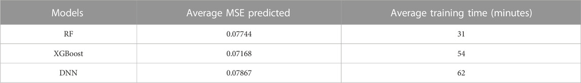
TABLE 1. Parameter adjustment results and training time of three models.

FIGURE 4

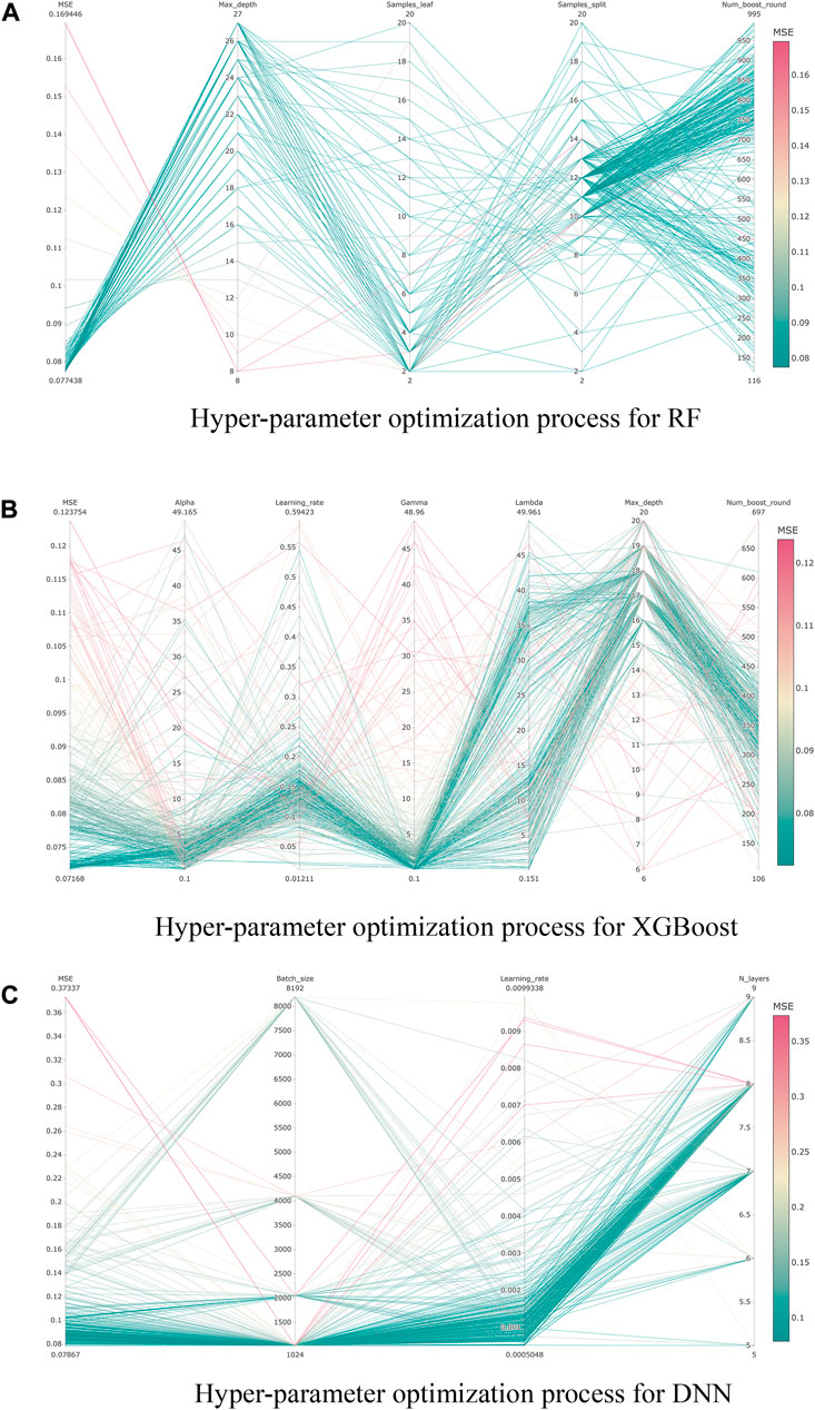
FIGURE 4. The Bayesian optimization process for hyper-parameters of the 3 ML models. (A)Hyper-parameter optimization process for RF, (B)Hyper-parameter optimization process for XGBoost, (C)Hyper-parameter optimization process for DNN.

3.4 Results for the four models

The traditional model by Yoojoong Choi et al. is used as the baseline model, and the results by the three proposed machine learning models are compared against it from the baseline model at periods of 0.01, 0.2, 1, and 3 s. The results are shown in Figure 5 where the horizontal axis is the actual Amp while the vertical axis is the predicted Amp. For further observing the prediction error of the model, we calculate the residual and the result is shown in Figure 6, where the residual can be calculated based on Eq. 13 which represents the model prediction error. As can be seen clearly from Figures 5, 6, the results from the three machine learning models show much less scattering and smaller residual, indicating better accuracy than it by the traditional approach. To further analyze the prediction accuracy of the three proposed models, R² and mean absolute error (MAE) are used to assess the three models for the training, testing and validation datasets. The results are shown in Figure 7, where R² represents the ratio of explainable portion in the overall squared summation divided by the predicted squared summation. The closer R² is to 1, the better the prediction results. R² and MAE can be expressed in the following equations.

${\mathit{R}}^{\mathbf{2}}=\mathbf{1}-\frac{{\sum }_{\mathit{i}=\mathbf{0}}^{\mathit{N}}{\left({\mathit{y}}_{\mathit{i}}-{\check{\mathit{y}}}_{\mathit{i}}\right)}^{\mathbf{2}}}{{\sum }_{\mathit{i}=\mathbf{0}}^{\mathit{N}}{\left({\mathit{y}}_{\mathit{i}}-\overline{{\mathit{y}}_{\mathit{i}}}\right)}^{\mathbf{2}}}(11)$

$\left.\mathit{M}\mathit{A}\mathit{E}=\frac{\mathbf{1}}{\mathit{N}}{\sum }_{\mathit{i}}^{\mathit{N}}\left({\mathit{y}}_{\mathit{i}}-{\check{\mathit{y}}}_{\mathit{i}}\right.\right)(12)$

$\mathbf{R}\mathbf{e}\mathbf{s}\mathbf{i}\mathbf{d}\mathbf{u}\mathbf{a}\mathbf{l}={\mathit{y}}_{\mathit{i}}-{\check{\mathit{y}}}_{\mathit{i}}(13)$

where $\mathit{N}$ represents the number of samples, ${\mathit{y}}_{\mathit{i}}$ is the object value of the $\mathit{i}$-th sample, ${\check{\mathit{y}}}_{\mathit{i}}$ is the predicted value of the $\mathit{i}$-th sample, and $\overline{{\mathit{y}}_{\mathit{i}}}$ is the mean value of the object value.

FIGURE 5

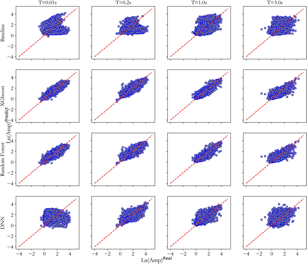
FIGURE 5. The prediction performance of four methods on validation dataset (The closer the scatter distribution is to the 1:1 line, the better the prediction results).

FIGURE 6

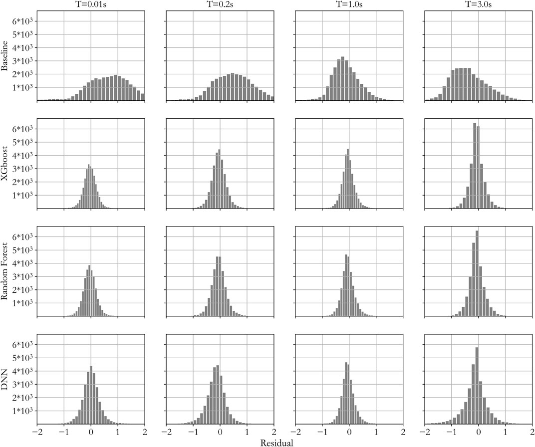
FIGURE 6. The prediction residual of four methods on validation dataset.

FIGURE 7

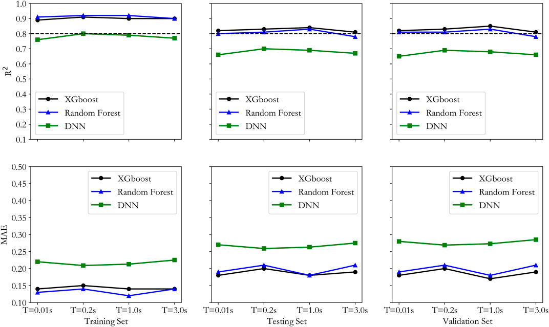
FIGURE 7. R² and MAE distribution of the three machine learning models for training, testing and validation datasets.

From the R² distribution in Figure 7 it can be concluded that DNN has smaller values than the values by both XGBoost and RF for training, testing and validation datasets. RF has higher R² value than it by XGBoost for the training dataset, but lower values for both the testing and validation datasets, indicating an overfitting trend by the RF model, which may lead to less generalization capability in future predictions. From the MAE distribution in Figure 7, it can be seen that DNN has the highest values in all three datasets, and RF has lower MAE than XGBoost for the training dataset, but it has higher MAE than XGBoost for both the testing and validation datasets. Based on the above observation, it can be concluded that the DNN model performed the worst, and RF model showed some over-fitting tendency, while the XGBoost model performed the best in predicting the site amplification factor.

To further study the generalization capability of the proposed XGBoost model, 6 events with different Vs30 values outside the training dataset were chosen to verify the amplification prediction results, as shown in Figure 8. As can be seen from Figure 8, for different Vs30, the predicted amplification factor is pretty close to the actual ratio, indicating good stability and generalization capability of the proposed model.

FIGURE 8

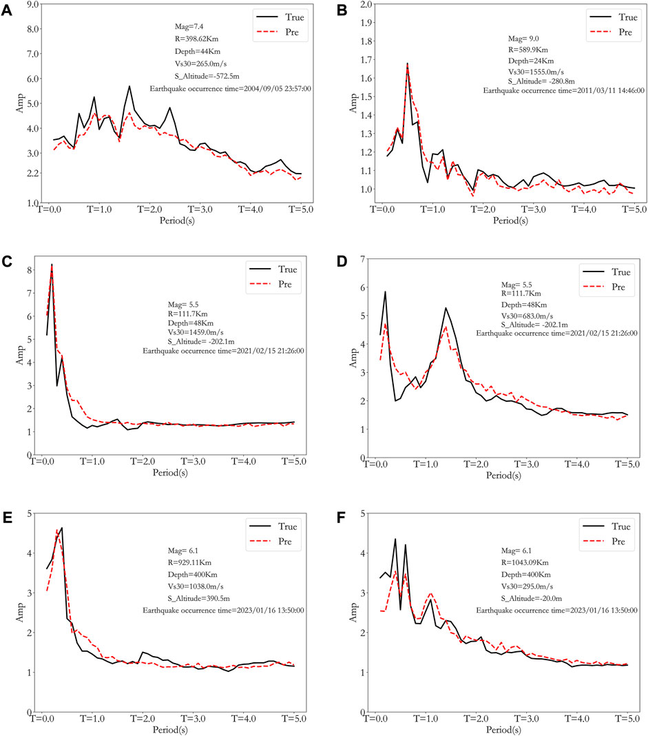
FIGURE 8. Generalization testing of actual events with different Vs30 (black line is the actual amplification while the red dashed line is the predicted amplification). The A−F figures represent seismic motion prediction validations for different earthquake events and site conditions, with earthquake events and site conditions presented as legends in each figure.

4 Explanation of the predicted results

Although machine learning has been increasingly applied in many areas with great success, it is still considered a “black box” approach with little reasonable explanation of the results. In this study the SHAP approach is introduced to explain the prediction models proposed. SHAP was originally constructed by Lundberg (Akiba et al., 2019) in 2017 as an explanation model, and its core is to calculate the contribution (SHAP values) of each feature parameter based on collaborative game theory to reflect the contribution of each parameter in the prediction. The calculation of SHAP value can be expressed in the following.

${\mathit{S}\mathit{H}\mathit{A}\mathit{P}}_{\mathit{f}\mathit{e}\mathit{a}\mathit{t}\mathit{u}\mathit{r}\mathit{e}}\left(\mathbf{x}\right)={\displaystyle \sum }_{\mathit{s}\mathit{e}\mathit{t}:\mathit{f}\mathit{e}\mathit{a}\mathit{t}\mathit{u}\mathit{r}\mathit{e}\in \mathit{s}\mathit{e}\mathit{t}}{\left[\left|\mathbf{s}\mathbf{e}\mathbf{t}\right|*\left(\begin{array}{c}\mathbf{F}\\ \left|\mathit{s}\mathit{e}\mathit{t}\right|\end{array}\right)\right]}^{-\mathbf{1}}\left[{\mathbf{y}}_{\mathit{s}\mathit{e}\mathit{t}}\left(\mathbf{x}\right)-{\mathbf{y}}_{\mathit{s}\mathit{e}\mathit{t}\backslash \mathit{f}\mathit{e}\mathit{a}\mathit{t}\mathit{u}\mathit{r}\mathit{e}}\left(\mathbf{x}\right)\right](14)$

where ${\mathbf{y}}_{\mathit{s}\mathit{e}\mathit{t}}\left(\mathit{x}\right)$ represents the model prediction when feature parameters are $\mathit{s}\mathit{e}\mathit{t}$ and $\mathbf{F}$ is the feature number.

For assembled tree models, SHAP method considers each feature parameter as a contributor, and the summation of contribution value from every parameter will lead to the final prediction assessment, as in the following (Lundberg and Lee, 2017):

$\mathit{y}={\mathbf{S}\mathbf{H}\mathbf{A}\mathbf{P}}_{\mathbf{0}}+{\sum }_{\mathit{i}=\mathbf{1}}^{\mathit{F}}{\mathit{S}\mathit{H}\mathit{A}\mathit{P}}_{\mathit{i}}(15)$

where $\mathit{y}$ is the predicted result by the model, and ${\mathbf{S}\mathbf{H}\mathbf{A}\mathbf{P}}_{\mathbf{0}}$ is the average prediction for all samples in the training dataset. ${\mathit{S}\mathit{H}\mathit{A}\mathit{P}}_{\mathit{i}}$ represents the SHAP value of the $\mathit{i}$-th feature parameter.

It should be noted that the effect of each feature parameter on the prediction has been studied in the past (Liu and Lei, 2005), but those studies did not consider the coupling effect of other feature parameters in the analysis. Based on collaborative game theory, SHAP approach can well represent the contribution by each feature parameter via SHAP value in the prediction results accounting for the coupleinge effect of feature parameters, and the contribution can be both positive and negative, thus well suited for explaining the prediction results (Zhang, 2020).

4.1 Contribution of each feature parameter

As explained in previous sections, XGBoost performed the best in the prediction, therefore it was selected to predict site amplification factor at 6 periods (0.01, 0.2, 0.6, 1, 2, and 3 s) and the corresponding SHAP values were calculated. For observation of the relationship between feature parameter and SHAP value, scattering plots were provided in Figure 9 for all 6 parameters at the 6 periods. From Figure 9 we can make the following observations.

1. SHAP value increases with Vs30 when Vs30 is small, but decreases when Vs30 is large, representing a negative correlation between SHAP value and Vs30. This negative trend increases with increasing period value. The positive correlation when Vs30 is small indicates that the predicted value for soft soil sites is bigger than actual value, and this over prediction is worse for longer periods. This observation is comparable to the conclusions in previous studies (Emel et al., 2014; Wojtuch et al., 2021), validating the results by this study and providing an evidence to show that SHAP analysis can well explain the model results.

2. There is generally a negative correlation between Mag and its SHAP value, representing over prediction by the model for smaller earthquakes.

3. There is no clear correlation trend between station altitude and its SHAP value when the period is short (0.01 and 0.2 s). When the period increases, the SHAP value is big when the altitude is small, and the SHAP value increases with decreasing station altitude, representing over prediction at low altitude for long periods.

4. There is obvious negative correlation between bedrock acceleration (Acc_rock) and SHAP value, which means that the model overpredicts the site amplification when Acc_rock is small but underestimates the amplification when Acc_rock is big. This observation is also supported by results by Beresnev (Walling et al., 2008), which may be because of non-linear effect of the site.

5. From the perspective of SHAP calculation, the SHAP values for Depth and R do not show a particularly obvious trend.

FIGURE 9

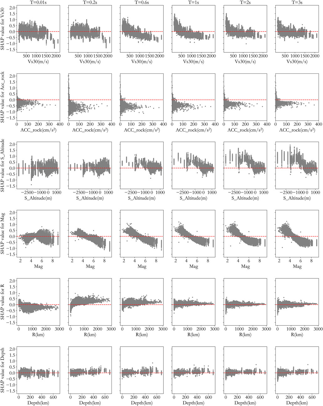
FIGURE 9. Scattering plots for feature parameters and their corresponding SHAP values.

4.2 Feature parameter importance

The SHAP value analysis has provided a good picture of the impact by each feature parameter, and to further quantify the impact of each parameter on the prediction results, importance analysis was performed for all the feature parameters in this study. In a typical XGBoost model, importance can be ranked using different measures (Gain, Cover, Weight) but the conclusion can be different if using different measures, so it is hard to decide which measure is the best for application. Since SHAP value represents the contribution of each feature parameter on the prediction result, we can use the average of the SHAP value to objectively represent the importance of each feature parameter and rank the absolute mean SHAP value to decide on the importance of each parameter. The results are shown in Table 2. The same results are graphically represented in Figure 9 for better comprehension. As can be seen from both Table 2 and Figure 10 Vs30, Mag, S_Altitude and Acc_rock have relatively large influence on the prediction results while R and Depth show less influence with Vs30 having the largest impact and Depth having the least impact. These results may serve as good reference for future site amplification studies.

TABLE 2

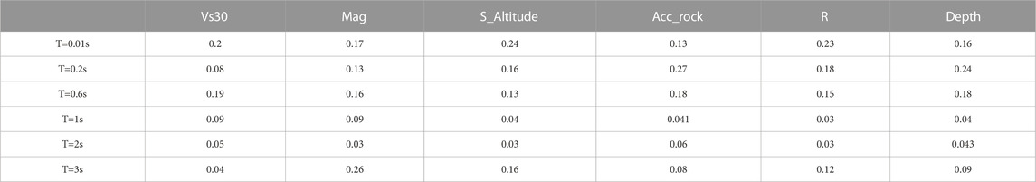
TABLE 2. Average SHAP value of each feature parameter at different periods.

FIGURE 10

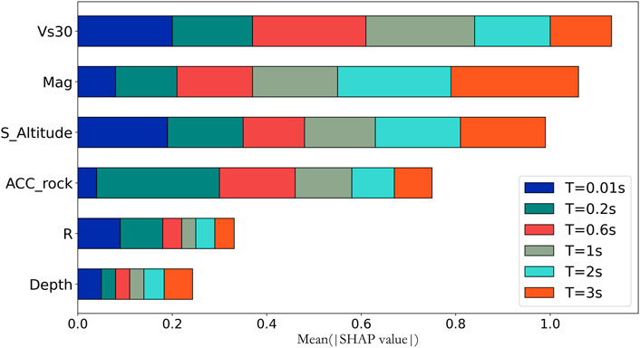
FIGURE 10. Feature importance ranking.

5 Conclusion

Based on the observed ground motion between 1997 and 2019 and station information from the KiK-net, a large database was assembled that included both the site amplification factor and 6 feature parameters. Three prediction models for site amplification factor based on machine learning were proposed and prediction results were compared against the result by a traditional approach at 6 different periods. Extensive analysis was conducted to find the best prediction model. SHAP analysis was used on the XGBoost model to provide better explanation of the prediction results and assess the impact and importance of the 6 feature parameters at 6 different periods. The following observations can be made based on this study.

1. In terms of predicting site amplification effect, machine learning algorithms are significantly better than traditional regression methods. Among the three machine learning approaches studied, XGBoost performs the best, followed by RF and DNN.

2. Comparison with the actual ground motion records for site amplification verifies the performance of the XGBoost prediction model, demonstrating huge potential of machine learning in site amplification factor prediction.

3. In the SHAP analysis, Vs30, Acc_rock and Mag are significantly negatively correlated with the predicted value, and S_Altitude is negatively correlated for large periods.

4. Of the 6 feature parameters, Vs30 has the largest impact on the prediction results, followed by Mag, S_Altitude, Acc_rock, R and Depth of the hypocenter.

These conclusions can be used to better quantify the effect of site condition and provide reference for future studies on site conditions.

Data availability statement

Publicly available datasets were analyzed in this study. This data can be found here: https://www.doi.org/10.17598/NIED.0004 https://pan.baidu.com/

Author contributions

XW, ZW, and JW participated in the conception and design of the study and wrote the first draft. PM, HD, and ZL wrote sections of the manuscript. All authors contributed to manuscript revision, read, and approved the submitted version.

Funding

This study is funded by National Natural Science Foundation of China (51978634) and Scientific Research Fund of Institute of Engineering Mechanics, China Earthquake Administration (Grant No. 2021B09).

Acknowledgments

The authors are grateful to NIED for its ground motion database, and to Google for its TensorFlow package used in this study.

Conflict of interest

Authors ZW and JW were employed by CEAKJ ADPRHexa Inc.

The remaining authors declare that the research was conducted in the absence of any commercial or financial relationships that could be construed as a potential conflict of interest.

Publisher’s note

All claims expressed in this article are solely those of the authors and do not necessarily represent those of their affiliated organizations, or those of the publisher, the editors and the reviewers. Any product that may be evaluated in this article, or claim that may be made by its manufacturer, is not guaranteed or endorsed by the publisher.

References

Abrahamson, N. A., and Silva, W. J. (1997). Empirical response spectral attenuation relations for shallow crustal earthquakes. Seismol. Res. Lett. 68 (1), 94–127. doi:10.1785/gssrl.68.1.94

CrossRef Full Text | Google Scholar

Akiba, T., Sano, S., and Yanase, T. (2019). “Optuna: A next-generation hyperparameter optimization framework,” in Proceedings of the 25th ACM SIGKDD international conference on knowledge discovery & data mining, 2623–2631.

Google Scholar

Bala, A., Grecu, B., Ciugudean, V., and Raileanu, V. (2009). Dynamic properties of the quaternary sedimentary rocks and their influence on seismic site effect: Case study in bucharest city, Romania. Soil Dyn. Earthq. Eng. 29 (1), 144–154.

CrossRef Full Text | Google Scholar

Bommer, J. J., and Martinez-Pereira, A. (2000). “Strong-motion parameters: Definition, usefulness andpredictability,” in Proc. of the 12th World Conference on Earthquake Engineering Auckland, New Zealand.

Google Scholar

Boore, D. M., Fumal, T. E., and Joyner, W. B. (1997). Equations for estimating horizontal response spectra and peak acceleration from western north American earthquakes: A summary of recent work. Seismol. Res. Lett. 68 (1), 128–153. doi:10.1785/gssrl.68.1.128

CrossRef Full Text | Google Scholar

Boore, D. M. (2004). Estimating s(30) (or NEHRP site classes) from shallow velocity models (depths < 30 m)[J]. Bull. Seismol. Soc. Am. 94 (2).

CrossRef Full Text | Google Scholar

Boore, D. M., Stewart, J. P., Seyhan, E., and Atkinson, G. M. (2014). NGA-West2 equations for predicting PGA, PGV, and 5% damped PSA for shallow crustal earthquakes. Earthq. Spectra 30 (3), 1057–1085. doi:10.1193/070113eqs184m

CrossRef Full Text | Google Scholar

Borcherdt, R. D., and Gibbs, J. F. (1976). Effects of local geological conditions in the San Francisco Bay region on ground motions and the intensities of the 1906 earthquake. Bull. Seismol. Soc. Am. 66 (2), 1170.

CrossRef Full Text | Google Scholar

Borcherdt, R. D. (1970). Effects of local geology on ground motion near San Francisco Bay. Bull. Seismol. Soc. Am. 60 (1), 29–61.

Google Scholar

Breiman, L. (2001). Random forests. Mach. Learn. 45 (1), 5–32. doi:10.1023/a:1010933404324

CrossRef Full Text | Google Scholar

Chen Longwei Chen Zhuoshi Yuan Xiaoming (2013). Site-specific amplification function assessment and variability analysis using KiK-Net single-station strong motion data. China Cicil Eng. J. 46, 141–145.

Google Scholar

Chen, T., and Guestrin, C. (2016). “Xgboost: A scalable tree boosting system,” in Proceedings of the 22nd acm Sigkdd International Conference on Knowledge Discovery and Data Mining, 785–794.

Google Scholar

Derras, B., Bard, P-Y., and Cotton, F. (2017). VS30, slope, H800 and f0: Performance of various site-condition proxies in reducing ground-motion aleatory variability and predicting nonlinear site response. Earth Planets Space 69 (1), 133. doi:10.1186/s40623-017-0718-z

CrossRef Full Text | Google Scholar

Dobry, R., Borcherdt, R., Crouse, C., Idriss, I. M., Joyner, W. B., Martin, G. R., et al. (2000). New site coefficients and site classification system used in recent building seismic code provisions. Earthq. Spectra 16 (1), 41–67. doi:10.1193/1.1586082

CrossRef Full Text | Google Scholar

Emel, S., Jonathan, P. S., and Eeri, S. (2014). Semi-empirical nonlinear site amplification from NGA-west2 data and simulations. Earthq. Spectra Prof. J. Earthq. Eng. Res. Inst. 30 (3), 1241–1256. doi:10.1193/063013eqs181m

CrossRef Full Text | Google Scholar

Gerolymos, N., and Gazetas, G. (2005). Constitutive model for 1-D cyclic soil behaviour applied to seismic analysis of layered deposits. Soils Found. 45 (3), 147–159. doi:10.3208/sandf.45.3_147

CrossRef Full Text | Google Scholar

Hamidreza, T., and Soleimani Kutanaei, S. (2015). Evaluation of effect of soil characteristics on the seismic amplification factor using the neural network and reliability concept. Arabian J. Geosciences 8 (6), 3881–3891. doi:10.1007/s12517-014-1458-z

CrossRef Full Text | Google Scholar

Harmon, J., Hashash, Y. M. A., Stewart, J. P., Rathje, E. M., Campbell, K. W., Silva, W. J., et al. (2019). Site amplification functions for central and eastern North America – Part II: Modular simulation-based models. Earthq. Spectra 35 (2), 815–847. doi:10.1193/091117eqs179m

CrossRef Full Text | Google Scholar

Hinton, G. E., Osindero, S., and Teh, Y. W. (2006). A fast learning algorithm for deep belief nets. Neural Comput. 18 (7), 1527–1554. doi:10.1162/neco.2006.18.7.1527

PubMed Abstract | CrossRef Full Text | Google Scholar

Idriss, I. M., and Seed, H. B. (1968). Seismic response of horizontal soil layers. Proc. ASCE 94 (4), 1003–1031. doi:10.1061/jsfeaq.0001163

CrossRef Full Text | Google Scholar

Jordan, M. I., and Mitchell, T. M. (2015). Machine learning: Trends, perspectives, and prospects. Science 349 (6245), 255–260. doi:10.1126/science.aaa8415

PubMed Abstract | CrossRef Full Text | Google Scholar

Kaveh, A., Bakhshpoori, T., and Hamze-Ziabari, S. M. (2016). Derivation of new equations for prediction of principal ground-motion parameters using M5′ algorithm. J. Earthq. Eng. 20 (6), 910–930. doi:10.1080/13632469.2015.1104758

CrossRef Full Text | Google Scholar

Liu, Huan, and Lei, Yu (2005). Toward integrating feature selection algorithms for classification and clustering [J]. IEEET rans Knowled geand Data Eng. 17 (4), 491–502.

Google Scholar

Lundberg, S. M., and Lee, S. I. (2017). “A unified approach to InterpretingModel predictions,” in Proceedings of Annual Conference onNeural Information Processing Systems, 4765–4774.

Google Scholar

Park, D., and Hashash, Y. M. A. (2008). Rate-dependent soil behavior in seismic site response analysis. Can. Geotechnical J. 45 (4), 454–469. doi:10.1139/t07-090

CrossRef Full Text | Google Scholar

Park, D., and Hashash, Y. M. A. (2004). Soil damping formulation in nonlinear time domain site response analysis. J. Earthq. Eng. 8 (2), 249–274. doi:10.1080/13632460409350489

CrossRef Full Text | Google Scholar

Roten, D., and Olsen, K. B. (2021). Estimation of site amplification from geotechnical array data using neural networks[J]. Bull. Seismol. Soc. Am. 111 (4).

Google Scholar

Roten, D., and Olsen, K. B. (2021). Estimation of site amplification from geotechnical array data using neural networks[J]. Bull. Seismol. Soc. Am. 111 (4), 1784–1794.

Google Scholar

Sadigh, K., Chang, C. Y., Egan, J. A., Makdisi, F., and Youngs, R. R. (1997). Attenuation relationships for shallow crustal earthquakes based on California strong motion data. Seismol. Res. Lett. 68 (1), 180–189. doi:10.1785/gssrl.68.1.180

CrossRef Full Text | Google Scholar

Seed, H. B., and Idriss, I. M. (1969). The influence of soil conditions on ground motions during earthquake[J]. J. Soil Mech. Found. Eng. Div. ASCE 94, 93–137.

Google Scholar

Seed, H. B., Romo, M. P., Sun, J. I., Jaime, A., and Lysmer, J. (1988). The Mexico earthquake of September 19, 1985: Relationships between soil conditions and earthquake ground motions [J]. Earthq. Spectra 4, 687–729. doi:10.1193/1.1585498

CrossRef Full Text | Google Scholar

Seyhan, E., and Stewart, J. P. (2014). Semi-empirical nonlinear site amplification from NGA-West2 data and simulations. Earthq. Spectra 30 (3), 1241–1256. doi:10.1193/063013eqs181m

CrossRef Full Text | Google Scholar

Walling, M., Silva, W., and Abrahamson, N. (2008). Nonlinear site amplification factors for constraining the NGA models. Earthq. Spectra 24 (1), 243–255. doi:10.1193/1.2934350

CrossRef Full Text | Google Scholar

Wojtuch, A., Jankowski, R., and Podlewska, S. (2021). How can SHAP values help to shape metabolic stability of chemical compounds? J. Cheminformatics 13 (1), 74–20. doi:10.1186/s13321-021-00542-y

CrossRef Full Text | Google Scholar

Yoojoong, C., and Jonathan, P. S. (2005). Nonlinear site amplification as function of 30 m shear wave velocity. Earthq. Spectra 21. doi:10.1193/1.1856535

CrossRef Full Text | Google Scholar

Zhang, L. (2020). Prediction of V _s30 in datong basin and amplification effect of site ground motion based on typical geological characteristics analysis. IOP Conf. Ser. Earth Environ. Sci. 455 (1), 012069. (11pp). doi:10.1088/1755-1315/455/1/012069

CrossRef Full Text | Google Scholar

Zhu, C., Cotton, F., Kawase, H., Haendel, A., Pilz, M., and Nakano, K. (2021). How well can we predict earthquake site response so far? Machine learning vs. Physics-based modeling. Earthq. Spectra 38 (2), 1047–1075. doi:10.1177/87552930211060859

CrossRef Full Text | Google Scholar