 Shufang Fan
 Wei Tang2,3
 Yanfei Wang
95% of researchers rate our articles as excellent or good
Learn more about the work of our research integrity team to safeguard the quality of each article we publish.
Find out more
ORIGINAL RESEARCH article
Front. Earth Sci. , 01 February 2023
Sec. Environmental Informatics and Remote Sensing
Volume 11 - 2023 | https://doi.org/10.3389/feart.2023.1050031
This article is part of the Research Topic Advances in Geophysical Inverse Problems View all 7 articles
X-Ray computed tomography is a non-destructive method that is used, among many applications, to study the size, shape, 3D structures and interconnections of pores in shale. We use phase retrieval methods to deal with the “edge enhancement” effect caused by phase shift. The process of phase retrieval can be described by the transport-of-intensity equation (TIE). But this is an ill-posed problem. The existing methods focus on phase retrieval in the frequency domain. To tackle the ill-posedness, we propose a new method whose main idea is to solve this problem in space domain with a regularization technique. We study a synthetic shale model and simulate the projection data. Then we apply three methods to retrieve the phase: conventional method in frequency domain, direct solving method and iterative Tikhonov regularization method in space domain. Finally, we use the standard filtered back-projection (FBP) method to present the outcome. By analyzing the results, we find advantages of the new method: more stability and fewer artifacts under noise perturbations. The study shows that relative errors of the new method are nearly 1% of that of the traditional method based on frequency domain, and hence the new method is promising for the practical data processing.
X-ray computed tomography (CT) is an important diagnostic approach in healthcare and is a non-destructive detecting technology. Due to its particular advantages, it is widely used in industry and medical imaging. CT relies on X-ray flux measurements from different angles to form an image. If the input X-ray photons are mono-chromatic, the X-ray intensities follow the Beer-Lambert law from the microscopic view (Natterer, 2001):
The common CT reconstruction algorithms can be divided into two categories: analytical methods and iterative methods (Natterer, 2001). In practice, we use methods like filtered back-projection algorithm (FBP) and the algebraic reconstruction technique (ART) correspondingly (Shepp and Logan, 1983; Gordon et al., 1970). The former one utilizes explicit formula which may cause ring-artifacts, whereas the latter can suppress some artifacts but requires longer computing time than the former one. Some commercially available CT scanners use fan-beam projections, but they are not applicable for the reconstruction of shale structure by using the synchrotron radiation-based X-ray CT. Synchrotron radiation allows us to select monochromatic X-ray beams from the full spectrum and conserve enough intensity for imaging. Because of the small size of the shale sample, parallel geometry can be used to conduct the experiment.
Conventional X-ray (CT) is based on the contrast of the absorption. However, a wide range of samples used in biology and material exhibit very weak absorption contrast, nevertheless can produce significant phase shifts in the X-ray beam (Bronnikov, 2006). When the distance between the sample and the CCD (CCD stands for “charged couple device”) becomes larger, the projected image becomes a mixture of the absorption-contrast image and the phase-contrast image. As for shale, it contains a lot of weak absorption organic materials which are similar with pores in the absorption-contrast image. Although the conventional X-ray CT algorithm may not distinguish the difference between the pore and weak absorption materials, the phase shift that X-ray undergoes when passing through the material may provide better image quality. Experiments have demonstrated that the intensity distribution changes a lot with different distances between the sample and the CCD (Bronnikov, 2006). This leads to a fact that the Radon transform cannot be used to simulate the practical process of the CT imaging exactly. Therefore, it is necessary to use the information about the phase. The “edge enhancement” effect caused by the phase shift will affect the final imaging (Chen et al., 2009). So we should use the phase information to reduce these artifacts.
X-ray phase contrast imaging has received much more attention in recent years, either in biomedical sciences (Bravin et al., 2013) or in material sciences (Mayo et al., 2012a; 2012b). The object can be depicted by its refractive index distribution,
The computational procedures of the X-ray phase contrast imaging can be outlined as follows (Lee, 2015).
• Phase retrieval
- Obtain the measured intensity function
- Calculate the Fourier transform of the measurement
- Apply a user-defined filter in frequency domain
- Perform the inverse Fourier transform of the filtered result
- Obtain the phase image through FBP or inversion
• Filtered back-projection (FBP)
- Calculate the Fourier transform of the phase
- Frequency filtering
- Calculate the inverse Fourier transform of the filtered result
- Back-projection
In above steps, the phase retrieval is used for dealing with the edge effect, while the FBP is used to present the image results.
There are two basic assumptions when we use the information of phase to retrieve the structure of the object: the absorption is negligible (
In this paper, we propose a new method based on space domain. In this new method, the problem can be expressed as
We will compare three methods: traditional transformed-based frequency-domain method, direct normal equation solving method (equaling to the least-squares method), and a posterior regularization method. To be simplicity in context, the above three methods are named as TFDM, LSM and PRM, respectively. These methods will be addressed in details in the following sections. Finally, some conclusions are given.
Let
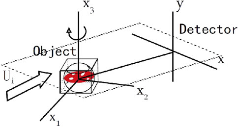
FIGURE 1. Coordinate system for the object and the plane of observation.
We assume that the source
where
The absorption function
where
where the double asterisk “**” denotes two-dimensional convolution and
where
where
The right-hand side of Eq. 8 is the observation, the left represents the effect caused by the phase. The conventional method to deal with this problem is to take the Fourier transform to both sides of the above equation to get (Paganin et al., 2002)
where
Instead of this final step, here we solve Eq. 8 directly in the space domain. To do so, we first build an operator equation to reformulate the Eq. 8 to get
where
All data are noisy, so Eq. 10 should be rewritten as:
Therefore we cannot guarantee that
where “
This method for solving ill-posed problems is called a Tikhonov regularizing method (Tikhonov and Arsenin, 1977; Wang et al., 2010). Tikhonov regularization means a variational approach based on minimization of a smoothing functional as follows (Xiao et al., 2003)
where
Numerical methods for minimizing
(1) Direct methods, i.e., solving an Euler equation:
(2) Iterative Tikhonov regularization methods: i.e., solving the above Euler equation iteratively with higher-order convergence rate.
(3) Optimization methods, i.e., solving an optimization problem
We will consider a posterior regularization method with optimal regularization parameter selection. Details will be given in the following section.
To simplify the notation, we denote the discrete form of the operator equation as
where
The coefficients
When the light travels through the air, we assume that the intensity at the detector equals the intensity at the object plane. This is the situation that happens at the boundary of the projection data. This condition means, the operator
where
Using this finite difference scheme, we can construct discrete operator
With the improvement of the spatial resolution, the condition number of the operator
The regularization method of solving Eq. 14 refers to minimize the following objective functional,
where
In order to verify the validity and advantages of the new algorithm, we carried out numerical simulations in the case of parallel-beam CT. The model we used is shown in Figure 2. In which, the grey values of the phantom represents the
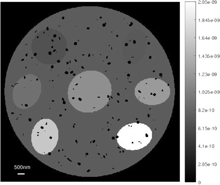
FIGURE 2. Linear absorption model.
The model’s main component is quartz, and the component percentages are listed as in Table 1.
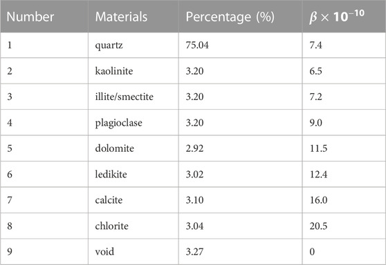
TABLE 1. Theoretical
The line integral projection is displayed as in Figure 3, where we discretize the model by decomposing it into
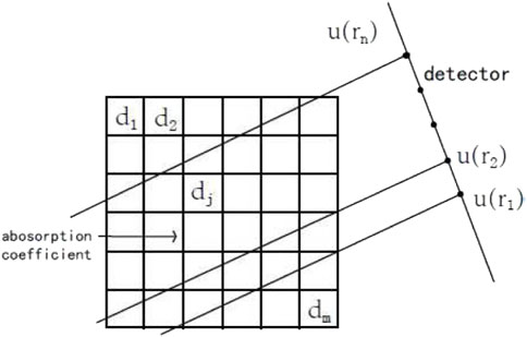
FIGURE 3. Acquisition geometry.
In our experiments, as mentioned before, we compare the three methods respectively: TFDM—the frequency domain method with phase retrieval, LSM—the direct method in space domain (without regularization), and PRM-the proposed regularization method in space domain.
First we consider the ideal case, i.e., the data is noiseless. As a comparison, we first use the FBP method to deal with the projection without considering phase property. The reconstruction result is illustrated in Figure 4. The Err will be 227.2 and we will only get some blurred information at the edge of the structure. Therefore, the reconstruction result is unsatisfactory. This indicates that the effect caused by the phase information is inevitable.
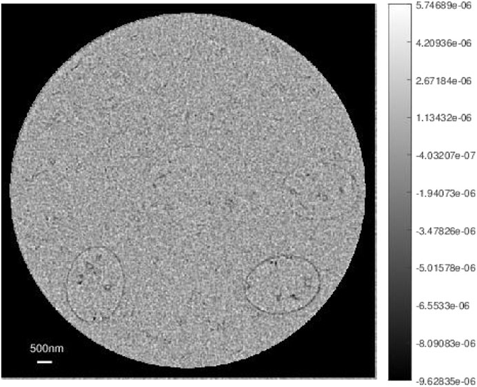
FIGURE 4. FBP result without phase retrieval.
We apply the aforementioned three methods to the phase retrieval problem. The reconstruction results are shown in Figures 5–7, respectively. The Errs for the three methods are 7.99, 0.018 and 0.018 correspondingly. The inversion results indicate that for noiseless data, the reconstructions from the direct method and the regularization method are similar, and are better than that of the frequency domain method.
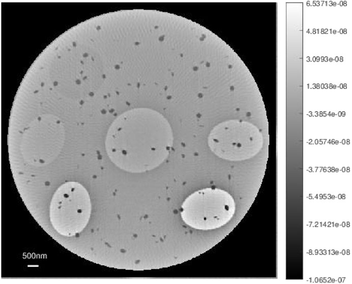
FIGURE 5. The inversion result using TFDM for noiseless data.
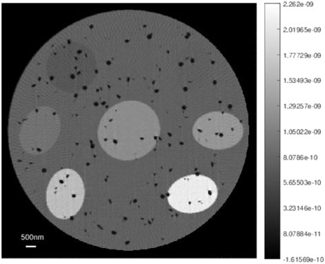
FIGURE 6. The inversion result using LSM for noiseless data.
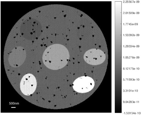
FIGURE 7. The inversion result using PRM for noiseless data.
A random noise with Gaussian distribution was added to the phantom projection. Two levels of noise were used, so that two new data sets were generated. First, we try to simulate the effect caused by small noise, where the noise-level equaling 0.1% is added to the true data. Figures 8–10 display the simulation results using the TFDM, LSM and PRM with 0.1% Gaussian noise in each case. The Errs for the three methods are 4.38, 1.51 and 0.0482, correspondingly.

FIGURE 8. The inversion result using TFDM for noisy data with noise-level 0.1%.
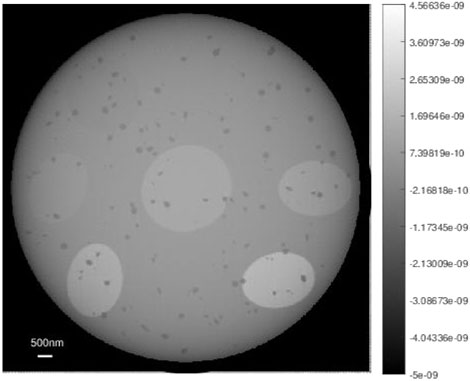
FIGURE 9. The inversion result using LSM for noisy data with noise-level 0.1%.
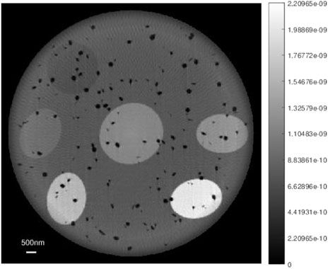
FIGURE 10. The inversion result using PRM for noisy data with noise-level 0.1%.
If we add large noise (noise-level = 1%), the results with the TFDM, LSM and PRM, are shown in Figures 11–13, respectively. The Errs for the three methods are 10.85, 14.02 and 0.0627 correspondingly. To quantitatively illustrate differences of the three methods, we draw a profile in Figure 14, which shows the results calculated by above mentioned three methods, in which the black line is the model parameter (true value), the red line is the result calculated by the regularization method (PRM) proposed in this paper, the green line is the result calculated by the LSM and the blue line is the result calculated by the TFDM in the frequency domain.
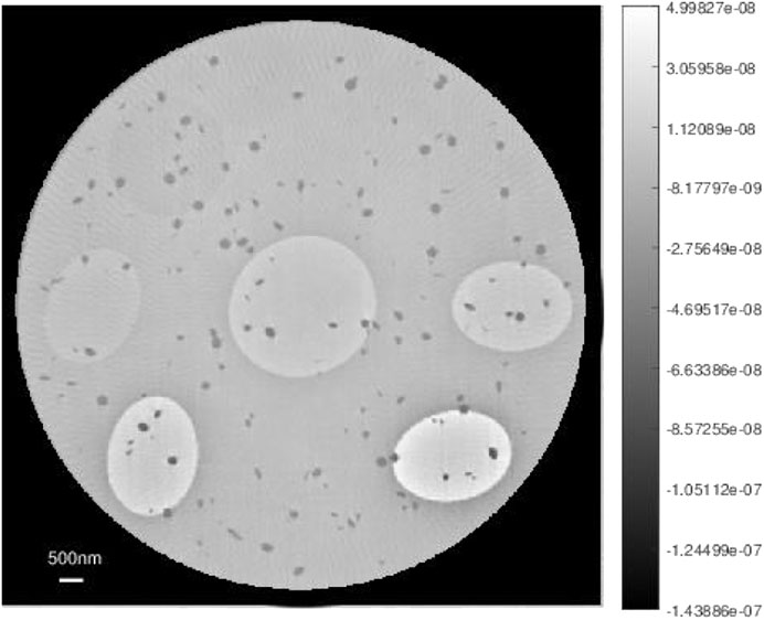
FIGURE 11. The inversion result using TFDM for noisy data with noise-level 1%.
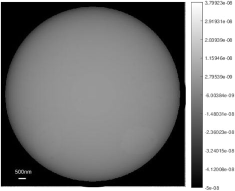
FIGURE 12. The inversion result using LSM for noisy data with noise-level 1%.
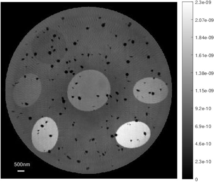
FIGURE 13. The inversion result using PRM for noisy data with noise-level 1%.
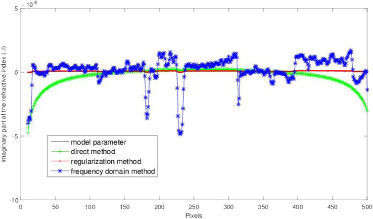
FIGURE 14. Comparison of three methods on their profiles for noisy data with noise-level 1%.
Due to the ill-posedness of the nano-scale CT imaging problem, the direct solution is not stable (LSM) when noise exists. When the noise level is 1%, it is even hard to get anything from the result as is shown in Figure 12. Under the same experiment condition, the signal-noise ratio will be low especially when the sample is in micro size. Therefore, even if the direct method has a fast computational speed, it is still hard to image well for the practical data, as noise always exists for practical measurements.
Even though the results given by the frequency domain method (TFDM) can show the structure information under some noise levels, if we observe a particular position where the pore located, the results, calculated by the frequency domain method, show significant difference. When the value of the model parameter is high, there exists serious artifact around them. So the results from the frequency method may be affected by the values of pixels around them. The worst thing for the frequency domain method is that its relative error is much higher than that of the proposed method in space domain. We also performed some numerical experiments under different situations (e.g., change the resolution, change the distance between sample and detector), the method we proposed behaved well.
An organic-rich shale sample is selected for this study. This sample is a Qiliao shale from Chongqing Shizhu-Qiliao profile belonging to the five peak group-Longmaxi (LMX) group, China. It is composed of quartz (71%), feldspar (8%), pyrite (3%), dolomite (4%), and illite-smectite-chlorite (14%). LMX formation shale at Shizhu-Qiliao outcrop mainly consisted of dark carbonaceous shale with pyrite and quartz veins. To carry out the experiment, the Nano-TXM samples were prepared by an FEI Helios Nano-Lab 600 DualBeam FIB-SEM. Nano-TXM experiments were carried out at beamline BL01B1, the National Synchrotron Radiation Research Center (NSRRC) in Hsinchu, Taiwan (Wang et al., 2016). Equipped with Zernike-phase-contrast capability, the instrument can take images of light materials such as biological specimens. The spatial resolution of the microscope is
As an illustration, the projection data of the first slice is shown in Figure 15. If we do not consider removal of phase effect, the inversion result is shown in Figure 16. With removal phase effect, we make a comparison of three methods: TFDM, LSM and PRM. As mentioned in theoretical simulations, the proposed regularization method (PRM) performs best. The inversion results using TFDM, LSM and PRM are shown in Figures 17–19, respectively. It is clear from Figure 19 that the high resolution result is obtained using PRM. To be focus, we zoomed the same part of each figure of the reconstruction in Figure 20, it clearly shows that the proposed regularization method (PRM) yields the better reconstruction result with high resolution. We also plot the histograms of the reconstruction results in Figure 21, where each output grayscale image has 64 bins. Finally, we patch all slices using PRM together to generate a three-dimensional in Figure 22. It illustrates that honeycomb coal-like pyrite and pores are observed clearly.
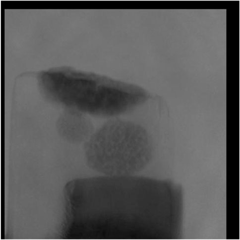
FIGURE 15. Projection data of the first slice.
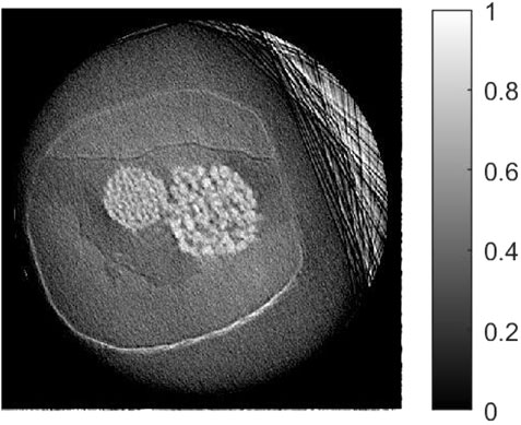
FIGURE 16. One slice of the reconstruction results: without phase removal.
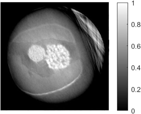
FIGURE 17. One slice of the reconstruction results: TFDM.

FIGURE 18. One slice of the reconstruction results: LSM.
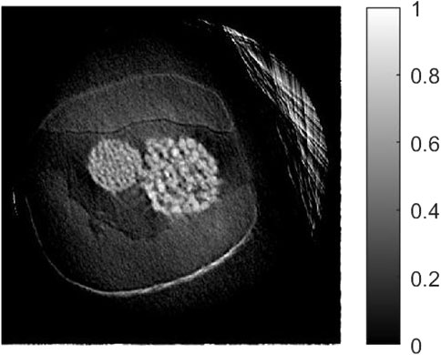
FIGURE 19. One slice of the reconstruction results: PRM.
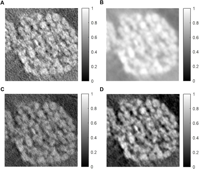
FIGURE 20. Comparison of reconstruction results with zoomed parts: (A) without phase removal, (B) TFDM, (C) LSM and (D) PRM.
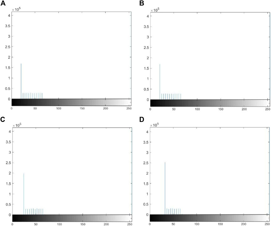
FIGURE 21. Histograms of reconstruction results: (A) without phase removal, (B) TFDM, (C) LSM and (D) PRM.
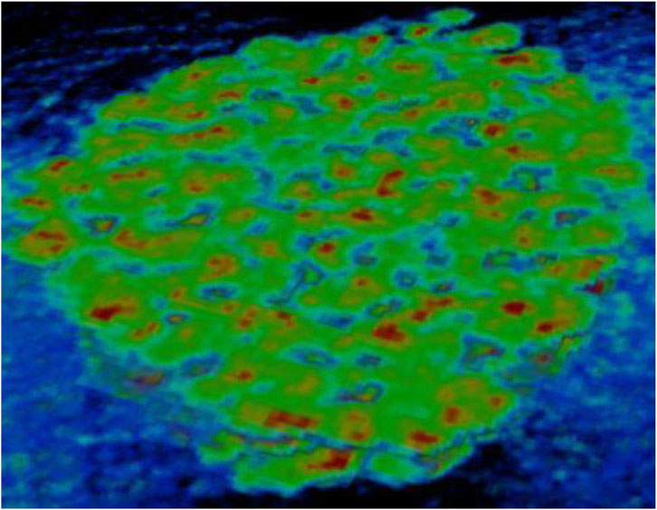
FIGURE 22. Three-dimensional display of the reconstruction results of PRM.
From methodological view of point, our method works for complex, finely layers systems prevalent in most shales, this is because, for shale samples, although the absorption of light cannot be ignored like biological samples, when the object leaves the receiving screen for a certain distance, the phase factor will cause certain interference to the projection data, forming an “edge enhancement” effect, which is necessary to combine the basic theory of phase contrast imaging to remove the interference of phase factors on the projection. Therefore, a phase retrieval model based on TIE equation in space domain is established. During solution of the TIE equation, since the discretization of differential operators leads to the instability of the problem, the regularization technique is employed, and a posterior regularization method in space domain (PRM) is proposed for solving the phase retrieval problem, meanwhile selection of an optimal posterior regularization parameter is adopted, which accelerates the convergence speed of the iterations. Due to an optimal regularization parameter is achieved, the solution reaches optimal. Comparison with the standard method in frequency domain (TFDM) and the direct method in space domain (LSM) shows that the regularization method yields an accurate reconstruction and is robust to noise. Though this method is theoretically sound, there is still a restriction: we assume that the ratio between the real and imaginary parts of the refraction coefficient is homogeneous which may not be practical. So when we want to deal with the real data, we should choose the suitable energy and ratio (between values
We remark that other imaging technique such as scanning electron microscopy equipped with a focused ion beam (FIB-SEM) can be used for nano-scale imaging of pore structures of shale. Though the resolution is high, it belongs to the destructive method. We believe that a combination of FIB-SEM (supplying high quality actual pore volume fraction) with nano-scale CT imaging will be a good choice for large amount of data analysis, e.g., employing the artificial intelligence technique, which will be also an interesting topic.
The original contributions presented in the study are included in the article/Supplementary Material, further inquiries can be directed to the corresponding author.
All authors listed have made a substantial, direct, and intellectual contribution to the work and approved it for publication.
The research is supported by Doctoral Scientific Research Foundation of Liaocheng University (Grant No. 318051911), the Innovation Research Program of the Chinese Academy of Sciences (Grant No. ZDBS-LY-DQC003) and the key program IGGCAS-2019031.
We are grateful for constructive comments from four reviewers and the editor, which improve the quality of the paper. The Center of Big Data and AI in Earth Sciences of IGGCAS in supplying facilities for simulation and practical data processing is also acknowledged.
The authors declare that they have no known competing financial interests or personal relationships that could have appeared to influence the work reported in this paper.
All claims expressed in this article are solely those of the authors and do not necessarily represent those of their affiliated organizations, or those of the publisher, the editors and the reviewers. Any product that may be evaluated in this article, or claim that may be made by its manufacturer, is not guaranteed or endorsed by the publisher.
Beltran, M. A., Paganin, D. M., Uesugi, K., and Kitchen, M. J. (2010). 2D and 3D X-ray phase retrieval of multi-material objects using a single defocus distance. Opt. Express. 18, 6423–6436. doi:10.1364/OE.18.006423
Bravin, A., Coan, P., and Suortti, P. (2013). X-Ray phase-contrast imaging: From pre-clinical applications towards clinics. Phys. Med. Biol. 58, 1–35. doi:10.1088/0031-9155/58/1/R1
Bravin, A. (2003). Exploiting the X-ray refraction contrast with an analyzer: The state of the art. J. Phys. 36, A24–A29. doi:10.1088/0022-3727/36/10A/306
Brenner, H. (1952). On the asymptotic evaluation of diffraction integrals with a special view to the theory of defocusing and optical contrast. Physica 18, 469–485. doi:10.1016/S0031-8914(52)80079-5
Bronnikov, A. V. (2006). Phase-contrast CT: Fundamental theorem and fast image reconstruction algorithms. Proc. Spie. 6318, 63180Q. doi:10.1117/12.679389
Bronnikov, A. V. (1999). Reconstruction formulas in phase-contrast tomography. Opt. Commun. 171, 239–244. doi:10.1016/S0030-4018(99)00575-1
Bronnikov, A. V. (2002). Theory of quantitative phase-contrast computed tomography. J. Opt. Soc. Am. A 19, 472–480. doi:10.1364/JOSAA.19.000472
Chen, R. C., Yangle, W., Tiqiao, X., Huitong, X., Zhou, G., and Deng, B. (2009). Preliminary results for X-ray phase contrast micro-tomography on the biomedical imaging beamline at SSRF. Nucl. Phys. 32, 241–245. doi:10.1088/1674-1137/33/8/010
Fan, S. F., Ma, Q. H., and Wang, Y. F. (2006). A new method for choosing regularization parameter with perturbed operator and noisy data. J. Beijing Normal Univ. Nat. Sci. 42, 25–31. doi:10.1007/s10444-011-9203-6
Freeden, W., Nashed, M. Z., Sonar, T., and Heine, C. (2010). Handbook of geomathematics. Heidelberg, Germany: Springer.
Gordon, R., Bender, R., and Herman, G. T. (1970). Algebraic reconstruction techniques (ART) for three-dimensional electron microscopy and X-ray photography. J. Theor. Biol. 29, 471–481. doi:10.1016/0022-5193(70)90109-8
Lane, R. G., and Tallon, M. (1992). Wave-front reconstruction using a Shack-Hartmann sensor. Appl. Opt. 31, 6902–6908. doi:10.1364/AO.31.006902
Lee, P. C. (2015). Phase retrieval method for in-line phase contrast X-ray imaging and denoising by regularization. Opt. Express. 23, 100668–110679. doi:10.1364/OE.23.010668
Liu, H. Q., Wang, Y., Ren, Y., Xue, Y., He, Y., and Guo, H. (2012). Investigation on X-ray micro-computed tomography suitable for organic compound samples based on modified Bronnikov algorithm. Acta. Opt. Sin. 32, 320–326. doi:10.3788/aos201232.0434001
Mayo, S. C., Stevenson, A. W., and Wilkings, S. W. (2012a). In-line phase-contrast x-ray imaging and tomography for materials science. Mater 5, 937–965. doi:10.3390/ma5050937
Mayo, S. C., Tulloh, A. M., Trinchi, A., and Yang, Y. S. (2012b). Data-constrained microstructure characterisation with multi-spectrum X-ray micro-CT. Microsc. Microanal. 18, 524–530. doi:10.1017/S1431927612000323
Natterer, F. (2001). The mathematics of computerized tomography. New York, USA: Society for Industrial and Applied Mathematics.
Nesterets, Y. I., and Wilkins, S. W. (2008). Phase-contrast imaging using a scanning-double-grating configuration. Opt. Express. 16, 5849–5867. doi:10.1364/OE.16.005849
Olivo, A., Diemoz, P. C., and Bravin, A. (2012). Amplification of the phase contrast signal at very high x-ray energies. Opt. Lett. 37, 915–917. doi:10.1364/OL.37.000915
Paganin, D., Mayo, S. C., Gureyev, T. E., Miller, P. R., and Wilkins, S. W. (2002). Simultaneous phase and amplitude extraction from a single defocused image of a homogeneous object. J. Microsc. 206, 33–40. doi:10.1046/j.1365-2818.2002.01010.x
Shepp, L. A., and Logan, B. F. (1983). The Fourier reconstruction of a head section. J. Opt. Soc. Am. 73, 1434–1441. doi:10.1109/TNS.1974.6499235
Sixou, B. (2015). Regularization methods for phase retrieval and phase contrast tomography. Abstr. Appl. 1–11. doi:10.1155/2015/943501
Song, Y. F., Chang, C. H., Liu, C. Y., Chang, S. H., Jeng, U. S., Lai, Y. H., et al. (2007). X-ray beamlines for structural studies at the NSRRC superconducting wavelength shifter. J. Synchrotron Rad. 14, 320–325. doi:10.1107/S0909049507021516
Tang, W., and Wang, Y. F. (2017). Iterative regularization methods for phase retrieval TIE equation in space domain. Chin. J. Geophys. 60 (5), 1851–1860. doi:10.6038/cjg20170520
Teague, M. R. (1983). Deterministic phase retrieval: A green’s function solution. J. Opt. Soc. Am. 73, 1434–1441. doi:10.1364/JOSA.73.001434
Tikhonov, A. N., and Arsenin, V. Y. (1977). Solutions of ill-posed problems. New York, USA: John Wiley & Sons.
Wang, Y. D., Yang, Y., Liu, K., Ren, Y., Tan, H., and Deng, B. (2015). Quantitative and multi-scale characterization of pore connections in tight reservoirs with micro-CT and DCM. Bull. Mineral. Pet. Geochem. 34, 86–92. doi:10.3969/j.issn.1007-2802.2015.01.010
Wang, Y. F. (2007). Computational methods for inverse problems and their applications. Beijing, China: Higher Education Press.
Wang, Y. F., Fan, S. F., Leonov, A. S., Lukyanenko, D. V., Yagola, A. G., Wang, L. H., et al. (2020). Non-smooth regularization and fast optimization algorithm for micropore reconstruction of shale. Chin. J. Geophys. 63 (5), 2036–2042. doi:10.6038/cjg2020M0684
Wang, Y. F., and Tang, W. (2018). Method and device for nano-scale imaging based on spatial phase retrieval technique. Patent 2, ZL201610566803. doi:10.1016/j.ultramic.2011.10.012
Wang, Y. F., and Xiao, T. Y. (2001). Fast realization algorithms for determining regularization parameters in linear inverse problems. Inverse. Probl. 17, 281–291. doi:10.1088/0266-5611/17/2/308
Y. F. Wang, A. G. Yagola, and C. C. Yang (Editors) (2010). (Heidelberg, Germany: Springer).Optimization and regularization for computational inverse problems and applications.
Wang, Y., Pu, J., Wang, L. H., Wang, J. Q., Jiang, Z., Song, Y. F., et al. (2016). Characterization of typical 3D pore networks of Jiulaodong formation shale using nano-transmission X-ray microscopy. Fuel 170, 84–91. doi:10.1016/j.fuel.2015.11.086
Wu, X. Z., and Liu, H. (2005). X-ray cone-beam phase tomography formulas based on phase-attenuation duality. Opt. Express. 13, 6000–6014. doi:10.1364/OPEX.13.006000
Xiao, T. Y., Yu, S. G., and Wang, Y. F. (2003). Numerical methods for the solution of inverse problems. Beijing, China: Science Press.
Ye, L. L. (2013). X-ray phase contrast micro-tomography and its application in quantitative 3D imaging study of wild ginseng characteristic microstructures. Acta. Opt. Sin. 33, 365–370. doi:10.3788/AOS201333.1234002
A posterior selection of the regularization parameter.
The minimization problem (17) is equivalent to solving the linear equations:
where
(1) A prior way: it requires knowledge of some source condition about the solution, e.g.,
(2) A posterior way: we can choose an optimal parameter
We suppose the noise level
Since
The derivative of the non-linear function
where
To solve for the parameter
Thus we use the Newton iterative formula for the parameter
Having specified the system matrix
(1) Input initial values of the regularization parameter
(2) Solve the Eq. (A5) using the Gaussian eliminations;
(3) Compute the function values
(4) Compute the parameter
(5) If
(6) Output
Keywords: X-ray tomography, inversion, regularization, phase retrieval, shale nanopores
Citation: Fan S, Tang W, Wang Y and Nashed MZ (2023) Posterior regularization method for phase removal of shale nano-structure imaging in space domain. Front. Earth Sci. 11:1050031. doi: 10.3389/feart.2023.1050031
Received: 21 September 2022; Accepted: 16 January 2023;
Published: 01 February 2023.
Edited by:
Ali Khenchaf, UMR6285 Laboratoire des Sciences et Techniques de l'Information de la Communication et de la Connaissance (LAB-STICC), FranceReviewed by:
Ederli Marangon, Federal University of Pampa, BrazilCopyright © 2023 Fan, Tang, Wang and Nashed. This is an open-access article distributed under the terms of the Creative Commons Attribution License (CC BY). The use, distribution or reproduction in other forums is permitted, provided the original author(s) and the copyright owner(s) are credited and that the original publication in this journal is cited, in accordance with accepted academic practice. No use, distribution or reproduction is permitted which does not comply with these terms.
*Correspondence: Yanfei Wang, eWZ3YW5nQG1haWwuaWdnY2FzLmFjLmNu
Disclaimer: All claims expressed in this article are solely those of the authors and do not necessarily represent those of their affiliated organizations, or those of the publisher, the editors and the reviewers. Any product that may be evaluated in this article or claim that may be made by its manufacturer is not guaranteed or endorsed by the publisher.
Research integrity at Frontiers
Learn more about the work of our research integrity team to safeguard the quality of each article we publish.