 Zhengwei Fang
 Liqiang Zhang
 Shicui Yan2
- 1School of Geosciences, China University of Petroleum (East China), Qingdao, China
- 2Research Institute of Petroleum Exploration and Development, Shengli Oilfield, Dongying, China
- 3Sinopec Key Laboratory of Shale Oil/Gas Exploration and Production, Shengli Oilfield Branch, Dongying, China
- 4Shandong Provincial Key Laboratory of Unconventional Oil and Gas Exploration and Development, Dongying, China
- 5Key Laboratory of Sedimentary Simulation and Reservoir Evaluation, Sinopec Shengli Oilfield, Dongying, China
Lacustrine shale in continental rift basins is complex and features a variety of mineralogical compositions and microstructures. The lithofacies type of shale, mainly determined by mineralogical composition and microstructure, is the most critical factor controlling the quality of shale oil reservoirs. Conventional geophysical methods cannot accurately forecast lacustrine shale lithofacies types, thus restricting the progress of shale oil exploration and development. Considering the lacustrine shale in the upper Es4 member of the Dongying Sag in the Jiyang Depression, Bohai Bay Basin, China, as the research object, the lithofacies type was forecast based on two machine learning methods: support vector machine (SVM) and extreme gradient boosting (XGBoost). To improve the forecast accuracy, we applied the following approaches: first, using core and thin section analyses of consecutively cored wells, the lithofacies were finely reclassified into 22 types according to mineralogical composition and microstructure, and the vertical change of lithofacies types was obtained. Second, in addition to commonly used well logging data, paleoenvironment parameter data (Rb/Sr ratio, paleoclimate parameter; Sr %, paleosalinity parameter; Ti %, paleoprovenance parameter; Fe/Mn ratio, paleo-water depth parameter; P/Ti ratio, paleoproductivity parameter) were applied to the forecast. Third, two sample extraction modes, namely, curve shape-to-points and point-to-point, were used in the machine learning process. Finally, the lithofacies type forecast was carried out under six different conditions. In the condition of selecting the curved shape-to-point sample extraction mode and inputting both well logging and paleoenvironment parameter data, the SVM method achieved the highest average forecast accuracy for all lithofacies types, reaching 68%, as well as the highest average forecast accuracy for favorable lithofacies types at 98%. The forecast accuracy for all lithofacies types improved by 7%–28% by using both well logging and paleoenvironment parameter data rather than using one or the other, and was 7%–8% higher by using the curve shape-to-point sample extraction mode compared to the point-to-point sample extraction mode. In addition, the learning sample quantity and data value overlap of different lithofacies types affected the forecast accuracy. The results of our study confirm that machine learning is an effective solution to forecast lacustrine shale lithofacies. When adopting machine learning methods, increasing the learning sample quantity (>45 groups), selecting the curve shape-to-point sample extraction mode, and using both well logging and paleoenvironment parameter data are effective ways to improve the forecast accuracy of lacustrine shale lithofacies types. The method and results of this study provide guidance to accurately forecast the lacustrine shale lithofacies types in new shale oil wells and will promote the harvest of lacustrine shale oil globally.
1 Introduction
Shale oil has attracted increasing attention as an unconventional resource. It can be produced from both marine and lacustrine shales. Marine shale is generally developed in a stable and gentle tectonic environment, has a few types of lithofacies (Loucks and Ruppel, 2007; Abouelresh et al., 2020), and is widely distributed (Li et al., 2019). In comparison, lacustrine shale formed in a continental rift basin has various types of lithofacies owing to paleogeological conditions such as a relatively small lake area, multiple material sources, and frequent climate changes (Wang et al., 2016; Jia et al., 2018; Li et al., 2020). Moreover, the type and thickness of lithofacies change frequently across layers (Liang et al., 2017), which presents unprecedented challenges to the forecasting of favorable lithofacies types and the selection of shale oil targets (Cao et al., 2019). Conventional well logging interpretation can forecast shale mineral components by calibrating with X-ray mineral content analysis; however, it cannot accurately forecast the microstructure (mineral distribution and arrangement) of shales or find favorable lithofacies. The lithofacies type is mainly determined by mineralogical composition and microstructure, which not only determine shale oil reservoir performance but also affects the fracture characteristics of shales (Niu et al., 2023). The mineralogical composition and microstructure affect the pore development and the brittleness of shale; therefore, the accurate determination of lithofacies type is closely related to the target layer selection of shale oil horizontal wells and the design of hydraulic fracturing schemes.
Machine learning technology currently provides new ideas and methods to solve interpretation ambiguity and uncertainty in geological evaluations, which is a new field that urgently requires exploration (Zhou et al., 2018; Li et al., 2021). As available geological data grow exponentially, research on big data mining and machine learning in oil exploration and development is gradually increasing. Naeini and Prindle (2018) used examples to demonstrate the application of machine learning in petroleum geology research, such as document and image segmentation, well-logged facies recognition, petrophysical logging prediction, and fault interpretation. Bergen et al. (2019) systematically analyzed the application of data-driven machine learning methods in Earth science, and Alkinani et al. (2019) summarized the application of artificial neural networks in the oil and gas industry. Regarding mineral and complex lithology identification, some researchers have achieved good results using machine learning (Carey et al., 2015; Dev and Eden, 2019; Guo, 2021). Machine learning can also be used to identify the diagenetic facies of tight sandstone, with good results (Li et al., 2022; Zhang et al., 2022).
In shale research, machine learning has been used to identify marine shale lithofacies (Bhattacharya and Carr, 2019), sweet spots (Tahmasebi et al., 2017), reservoir potential (Ali et al., 2022), and total organic carbon content forecasts (Shi et al., 2016), and to model shale gas production (Kalantari-Dahaghi et al., 2015; Belyadi, 2021). However, no effective method or machine learning-based solution currently exists to forecast lacustrine shale lithofacies types in continental rift basins.
The Jiyang Depression is a typical Cenozoic continental rift basin in eastern China that is rich in shale oil, and many shale oil wells have been drilled with cores. Conventional logging interpretation methods to select target layers in the early stages of shale oil exploration are poor, and alternative methods for lithofacies types forecast and accurately identifying target layers are urgently needed. This study on the upper Es4 member of the Dongying Sag in the Jiyang Depression is based on core observation, thin-section identification, and elemental and well logging analysis. This work performed lithofacies type forecast modeling using machine learning methods, compared the modeling results, and discussed factors affecting the accuracy of lithofacies type forecasts. As the exploration area has sufficient test data to establish an effective learning sample database, this work provides guidance to forecast the lithofacies types of shale strata with strong heterogeneity.
2 Geological background
The Bohai Bay Basin is a continental rift basin located in eastern China and contains a series of Paleogene-rifted depressions, namely, the Liaohe, Liaodong Bay, Bozhong, Jiyang, Huanghua, Jizhong, and Linqing Depression (Figure 1A; Liang et al., 2016). Dongying Sag developed during the Cenozoic rifting stage, in the southeastern of the Jiyang depression of the Bohai Bay Basin, and covers an area of 5,700 km2. It can be subdivided into four subsags (Minfeng, Lijin, Niuzhuang, and Boxing subsags) by several normal faults and the central anticlinal belt (Figure 1B).
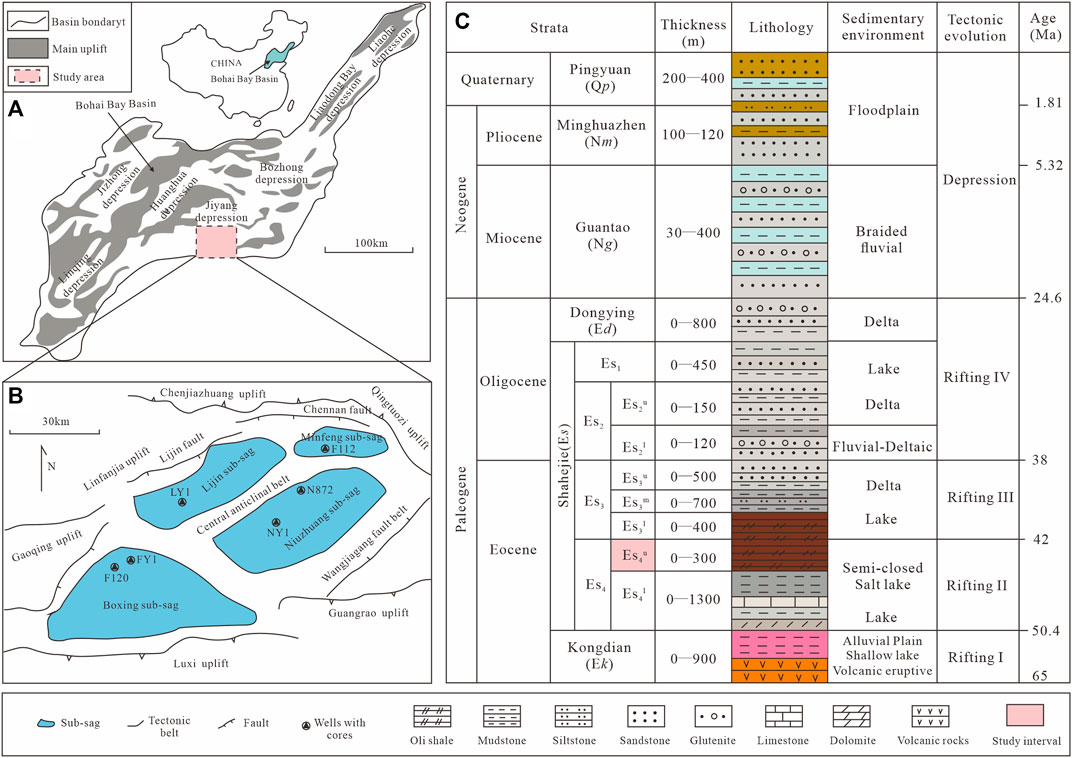
FIGURE 1. Location map (A), structural map and key well locations of the Dongying Sag, (B) and its stratigraphic column (C).
The Dongying Sag underwent rifting during the Paleogene period and a subsidence stage during the Neogene and Quaternary periods and was filled with a thick Cenozoic sediment sequence such as the Paleogene Kongdian (Ek), Shahejie (Es), and Dongying (Ed) formations (Figure 1C). The Es Formation is the main source rock and reservoir in the basin and is further divided into four members, Es4, Es3, Es2, and Es1 (from base to top). During the sedimentary period of Ek formation, the Dongying Sag was in the initial stage of rifting (Rifting I) due to crustal extension caused by an upwelling of the deep mantle and volcanic eruptions. The lacustrine basin had a shallow-water environment and a semi-arid climate, resulting in the deposition of red mudstone that contained gypsum salt. During the sedimentary period of Es4 (Rifting II), the climate gradually changed to a warm–semi-arid condition and the lake level rose, resulting in the deposition of black oil shales (Figure 1C). The upper part of the Es4 member (Es4u) consists of gray to black shales, calcareous shales, and mudstones. During the Es3 period, the lacustrine basin witnessed rift spreading (Rifting III), causing lake area expansion and water depth increase, resulting in the deposition of dark mudstones and calcareous shales. During the Es2 to Ed period, the lacustrine basin witnessed the shrinking of the rift (Rifting IV) and deposition of lacustrine delta strata.
At present, the shale oil wells drilled in the Es4u member of the Dongying Sag have achieved industrial oil flow. The member mainly comprises ∼300 m thick lacustrine shales and gradually becomes a very important exploration target for shale oil (Wang et al., 2019). During the early exploration for shale oil, a few exploratory wells (i.e., FY1, NY1, and LY1) (Figure 1B) drilled through the Es4u member, and a large amount of basic data was obtained. This study primarily focused on the Es4u member to forecast lacustrine shale lithofacies types based on machine learning.
3 Lithofacies classification
Lithofacies classification is the basis for building a learning sample database for machine learning. Recent studies have shown that the shale in the Dongying Sag can be divided into three major sedimentary categories (Wang et al., 2016). However, a unified understanding of the origin and sedimentary environment of each lithofacies is lacking. Well FY1 has a continuous core in the upper Es4 unit (from 3,245 to 3,440 m) of the Dongying Sag. In this study, the 195 m core was carefully observed and a total of 753 thin sections were made to identify the rock composition and microstructure, with an average of 1 thin section per 0.25 m. Core observation and thin-section identification of the typical components and sedimentary structures of shale can reflect the characteristics of the sedimentary environment. Finally, according to the characteristics of the mineralogical compositions and microstructures, the shale lithofacies in the upper Es4 unit of Well FY1 were divided into six major types and 22 minor types. A detailed description of this process is as follows.
The lithofacies deposited on lower coastal slopes include massive/layered silty fine sandstone (LL1), massive/layered cryptocrystalline granulated dolomite (LL2), and massive/layered cryptocrystalline granulated limestone (LL3). LL1 has a massive or layered structure and granular texture. The clastic particles are primarily very fine sand with a small amount of silt. The clastic components are mainly quartz and feldspar, as well as crystalline rock fragments, mica, and calcite. The intergranular fillings are mainly clay minerals, dolomite, and calcite. LL2 and LL3 have massive or layered structures and granular textures dominated by sand-sized grains and partial silt-sized grains. The grains include cryptocrystalline dolomitic and limy silt-to-sand sized allochem, oolites, and bioclasts with a certain amount of terrigenous clasts.
The lithofacies deposited in the upper shallow lake slope included layered silty mudstone muddy siltstone (US1), layered muddy cryptocrystalline dolomite bearing algal remains (US2), and layered ostracod-bearing muddy cryptocrystalline limestone (US3). US1 has a layered and partially laminated structure with relatively straight bedding and lamina boundaries. The silt is mixed with mud. US2 has a layered structure and is composed mainly of dolomite, calcite, mud, and small amounts of terrigenous clasts. The mud is uniformly mixed with dolomite. Deformed algal bands and algal remains filled completely by single-crystal calcite were also observed. US3 has a layered structure and is composed mainly of grains, calcite, mud, and silt. The grains are mainly ostracod fragments with a small amount of remaining microcrystalline-cryptocrystalline limy algal. The ostracod fragments show a significant directional arrangement.
The lithofacies deposited on the middle shallow lake slopes include layered mudstone (MS1), layered cryptocrystalline limestone (MS2), layered ostracod- and silt-bearing mudstone (MS3), and layered cryptocrystalline dolomite (MS4). MS1 has a layered structure and muddy texture. It is mainly composed of mud with a small amount of silt and occasional oriented ostracod fragments. MS2 and MS4 have layered structures. They are composed of cryptocrystalline lime or dolomite and a small amount of mud. MS2 and MS4 are generally homogeneous and not subjected to hydrodynamic action. MS3 has a layered structure and muddy texture. It is primarily composed of mud with silts and ostracod fragments oriented along the bedding plane.
The lithofacies deposited in the lower shallow lake slope include lenticular laminated limestone-mudstone (LS1), lenticular laminated dolomite-limestone (LS2), lenticular imbricate limy-silty-muddy peperite (LS3), and lenticular Ostracoda-bearing limestone-mudstone (LS4). LS1 exhibits a lenticular structure. Micritic or powder crystal limes are lenticular, banded, and wrapped in mud with small amounts of silt. LS2 also exhibits a lenticular structure. The micritic or powdered crystal limes are lenticular, banded, and wrapped in clay and dolomite layers. Dolomite displays a micritic texture with a uniform crystal size. LS3 also has a lenticular structure. The micritic or powdered crystal limes are lenticular, banded, and filled with or wrapped in mud and silt. LS4 features lenticular lamina. Micritic or powder crystal limes are lenticular, banded, and wrapped in mud containing a small amount of silt. Oriented ostracod fragments are also observed in LS4.
The lithofacies deposited in the semi-deep lake include laminated muddy cryptocrystalline limestone (SD1), laminated muddy sparite limestone (SD2), laminated muddy cryptocrystalline dolomite (SD3), and laminated dolomitic muddy cryptocrystalline limestone (SD4). SD1 and SD3 have laminated structures with fine, straight laminae. The lamination is mainly displayed in the interbedding of organic-rich clayey lamina and limy or dolomitic lamina. The laminae are evenly distributed with clear boundaries. The lamina is 0.05–0.15 mm thick. The limy and dolomitic materials have micritic or powder crystal textures. SD2 has the same structure and composition as SD1 but includes limy laminae with medium to fine crystal texture and a higher content of organic matter in the interbedded clayey laminae. The medium-to-fine crystal limy lamina was recrystallized from the micritic limy lamina. SD4 has a laminated structure. The three main types of laminae—limy, clayey, and dolomite mitochondrial laminae—show uneven thicknesses and distributions.
The lithofacies deposited in the deep lake include laminated organic-rich mudstone (D1), laminated lime-bearing mudstone (D2), laminated mudstone containing sparry calcite (D3), and laminated dolomitic mudstone (D4). D1 has a laminated structure and is mainly composed of clay minerals. The lamination is displayed in the interbedding of clayey and organic laminae, and the bedding or lamina interface is straight. D2 also has a laminated structure. The lamination is displayed as the interbedding of clayey and organic lamina, with a small amount of cryptocrystalline limy lamina unevenly distributed between the former types of laminae. The structure of D3 is like that of D1 but differs from that of D1 in the local distribution of leguminous coarse and chain-shaped fine crystal calcite along the lamina. Both leguminous and chain-shaped calcites were formed during diagenesis. Lastly, D4 also has a laminated structure. The bedding mainly consists of dolomite mitochondrial laminae. The dolomite presents a fine crystal and micritic texture and develops densely in the mitochondrial form, including some organic matter and clayey lamina.
The 22 lithofacies types varied in mineral compositions and structures (Figure 2). Typical microscopic images of the various lithofacies are shown in Figure 2. The laminated lithofacies deposited in a semi-deep lake (SD1–SD4) are the most favorable lithofacies to extract shale oil (Sun, 2017). Different sedimentary environments form shales with different components and structures, which function as the physical basis or mechanism to predict shale lithofacies.
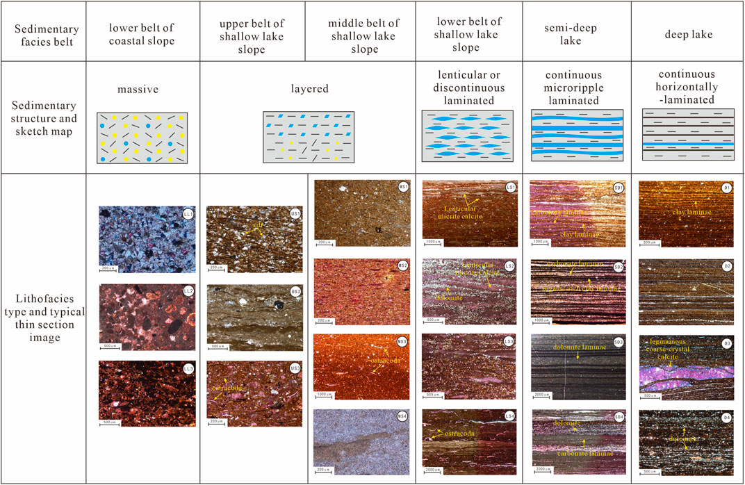
FIGURE 2. Lithofacies types of shale in the upper member of Es4 of the Dongying Sag.
In this study, the vertical lithofacies from 3,245 to 3,440 m in Well FY1 were distinguished using thin-section identification and color and structural changes in the continuous core section images (Figure 3A). The frequencies and thicknesses of the different lithofacies varied (Figure 3B). In the entire core section, LS1 was the thickest and had the second-largest frequency; MS1 was the second thickest and had the largest frequency; D2, LL1, LL2, LL3, LS2, LS4, MS2, MS4, and US2 had smaller thicknesses and frequencies; and the remaining lithofacies had medium thicknesses and frequencies.
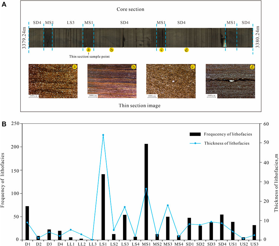
FIGURE 3. Example of vertical lithofacies division (A) and frequency and thickness statistics of different lithofacies types (B).
4 Data and methods
4.1 Data acquisition
Nearly all oil and gas exploration and development wells have acquired well logging data. Logging data lithology and lithofacies identification have wide applicability; therefore, samples from well logging data were preferred in this study. A total of 1,561 logging data sampling points exist in the upper Es4 of Well FY1, from 3,245 to 3,440 m, with a sampling interval of 0.125 m. Five logging parameters that are sensitive to shale lithology and lithofacies were selected as the sample sources, namely, natural gamma ray logging (GR), resistivity, acoustic slowness, density (DEN), and compensated neutron logging. All logging data were normalized by Shengli Logging Company before they were obtained. The relationship between well logging data and lithofacies was preliminarily analyzed, as shown in Figure 4. Different lithofacies have different ranges of GR values; a small portion has obvious differences, and a large portion has overlapping GR ranges (Figure 4A). Other logging responses exhibit similar characteristics. In the cross-plot of GR and DEN (Figure 4B), differentiation between the lithofacies was very low. With an increase in the number of lithofacies classifications, the difference in logging responses of various lithofacies decreases, and the difficulty of lithofacies prediction increases. The traditional method of attribute intersection is not sufficient to work with high-dimensional attributes because the attributes of various lithofacies are often intersectional or even inclusionary.
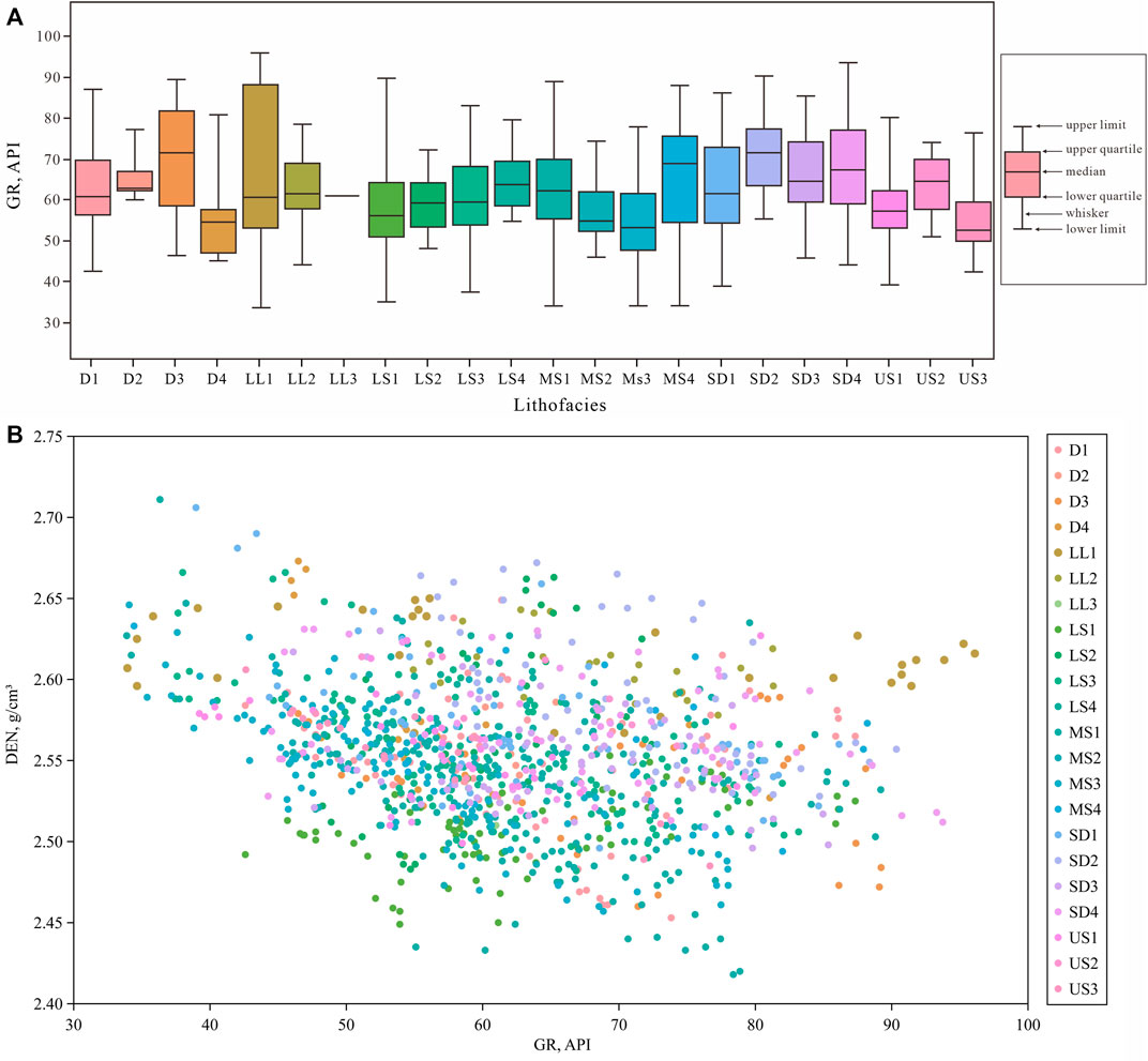
FIGURE 4. Boxplot of gamma-ray logging values for different lithofacies types (A) and cross-plot of DEN-GR (B).
In addition, because the components and sedimentary structures of shale are strongly related to the paleoenvironment (Croudace et al., 2015; Wang et al., 2021; Fu et al., 2018), paleoenvironmental parameters can reasonably be used to predict lithofacies. This is useful to determine differences between shale lithofacies. By testing the strength of the output signal, a portable X-ray fluorescence spectrum scanner (XRF) can qualitatively and semi-quantitatively analyze the chemical element compositions of sediments and obtain high-resolution, continuous element records. XRF is advantageous in that it is minimally destructive, convenient, and fast; it has been widely used to study sedimentary paleoenvironmental changes in sediments in lakes, oceans, rivers, and loess sedimentation (Tian et al., 2011). The present study used a handheld XRF (Bruker Company) on the core section of Well FY1 from 3,245 to 3,440 m using the general mode, 10 kV detection voltage, 0.15 mA current, 60 s detection time, and 4–15 cm sampling interval. A total of 2,334 data points were obtained, and major (Ca, Si, Al, Mg, Fe, K, etc.) and trace (Ti, Rb, Cr, Mn, Sr, p, Cu, Zr, etc.) elements were detected in more than 20 species. All elemental data obtained by XRF were normalized using Origin 9.0. Five paleoenvironmental parameters widely used to study sedimentary environments were obtained: the Rb/Sr ratio (paleoclimate parameter), Sr % (paleosalinity parameter), Ti % (paleoprovenance parameter), Fe/Mn ratio (paleo-water depth parameter), and P/Ti ratio (paleoproductivity parameter) (Fu et al., 2018; Liu et al., 2019; Yang et al., 2021). Lithofacies are the product of paleoenvironmental and diagenetic evolution, and the elements in shale are affected by both. The shale thickness in the study area reaches hundreds of meters, and the diagenesis process is in a closed system, hindering long-distance fluid migration and exchange. Therefore, the sedimentary environment is the main controlling factor for the composition and structure of shale in the study area. In addition, considering the influence of diagenesis, the selected paleoenvironmental parameters were elements with relatively slow migration rates in diagenetic evolution, which were often used as important indicators in previous research on the paleoenvironment of shale formation.
The sample distributions of different lithofacies are shown in Figure 5. Owing to the differences in thickness, the well logging and paleoenvironmental data quantity varied significantly for each lithofacies. In addition, owing to the detection limits of the XRF instrument, five paleoenvironmental parameters were incomplete at some depth points, resulting in slightly fewer paleoenvironmental parameter data points than logging data points.
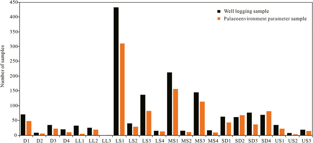
FIGURE 5. Sample quantities for different lithofacies types.
4.2 Sample extraction
Lithofacies predicted by well logging or paleoenvironmental parameter data should be matched one-to-one with the lithofacies according to depth. Two correspondence or sample extraction modes were used in this study: point-to-point and curve shape-to-point (Figure 6).
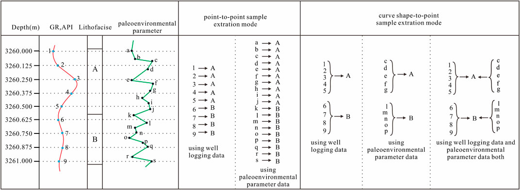
FIGURE 6. Sketch of point-to-point and curve shape-to-point sample extraction modes.
The point-to-point sample extraction mode is suitable for predicting lithofacies from either well logging or paleoenvironmental parameter data. The well logging sampling interval was 0.125 m. Thus, the data and corresponding lithofacies were extracted at 0.125 m intervals in the depth domain to form a one-to-one sample database. The sampling interval of the paleoenvironmental parameters was 0.05–0.15 m; thus, the paleoenvironmental parameters and corresponding lithofacies were extracted at the same intervals. The two sample databases must be used separately owing to the different sampling intervals, which prevented their fusion.
When predicting lithofacies using two sets of data, the curve shape-to-point sample data extraction mode must be used to obtain fusion information of the two types of data. We selected the 0.05 m sampling interval as the final sampling interval to extract the depth points. For each depth point, the nearest data points (selecting the three nearest paleoenvironmental parameter data points and the four nearest well logging data points) were acquired to represent the morphological characteristics of the sample values.
4.3 Selection of machine learning methods
Considering the heterogeneous distribution and quantity differences of the different lithofacies types, two machine learning methods were chosen: support vector machine (SVM) and extreme gradient boosting (XGBoost).
SVM is a representative machine learning method that has significant advantages in solving identification problems with small, non-linear, and highly dimensional sample sizes. Its main function is to identify the most important learning samples (called support vectors) that affect pattern judgment during training and then complete the data prediction based on these samples, thereby greatly improving fault tolerance and calculation efficiency (Suykens and Vandewalle, 1999; Vapnik, 1999). Li et al. (2019) analyzed the importance of machine learning methods in lithology identification and demonstrated the effectiveness of the SVM model. The theory and specific formula of the SVM are described in detail in Machine Learning in Action (Harrington, 2012), and a principal map of the SVM is shown in Figures 7A,B. An SVM is essentially a classification method with the function:
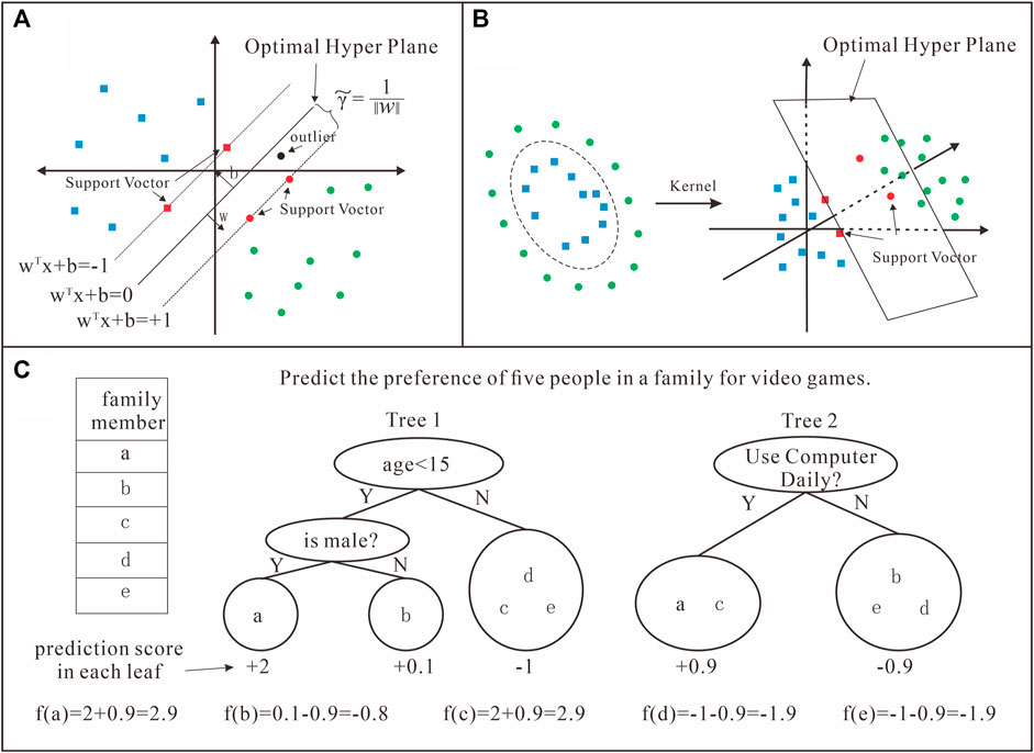
FIGURE 7. Principle sketch map of support vector machine (SVM); two-dimensional linear classification (A); two-dimensional non-linear classification (B) (quote from Harrington (2012) and modified locally) and extreme gradient boosting (XGBoost); the final prediction for a given example is the sum of the predictions from each tree (C) (quote from Chen and Guestrin (2016)).
The learning goal of the SVM is to identify a hyperplane in the n-dimensional data space. The equations for this hyperplane can be expressed as
Because of outliers (data points far from the normal position), the slack variable
where C is a hyperparameter >0, called the penalty parameter, which controls the weight between the two items in the objective function; namely, finding the hyperplane with the largest margin and ensuring minimal deviation of data points.
Kernel functions
When given values for C and
XGBoost can solve related problems using less data. XGBoost is a distributed general gradient-boosting library that improves the gradient-boosting decision tree and aims for efficiency, flexibility, and portability. The calculation efficiency of the XGBoost model generally decreases with increasing numbers of independent variables in the sample. When considering more independent variables, several variables are randomly selected to reorganize the learning samples so that the model can quickly process smaller learning samples (Liu et al., 2021). XGBoost avoids overfitting with high probability during the training process, thereby ensuring its reliability. Owing to the integration of parallel computing technology, the calculation efficiency of the model does not decline significantly with increasing training sample size (Zhou et al., 2020; Den et al., 2019). The theory and specific formula of XGBoost are described in detail by Chen and Guestrin (2016), and a principal sketch map of XGBoost is shown in Figure 7C. The core concept of XGBoost is to constantly add trees and split features to grow a tree. By adding a tree each time, a new function
The prediction function of XGBoost model is defined as
where
The loss function L is represented by the predicted value
where n is the number of samples. The loss function represents deviation in the model, and the variance is determined by the regular term Ω that suppresses the model’s complexity. The objective function Obj can be defined as
where T represents the number of leaf nodes, ω is the leaf weight value, γ is the penalty factor of the leaf tree, and λ is the leaf weight penalty factor. For each step, the loss function values must be calculated, and the objective function to obtain
K-fold cross-validation was selected to optimize the model parameters in the present study. This robust hyperparameter optimization method identifies a hyperparameter value to optimize the model generalization performance, effectively utilizing limited data and making the evaluation results as close as possible to the performance of the model in the test set. The training set in our study was divided into five parts. In the cross-validation process, we selected one part for training and the other four parts for verification, cycle training, and testing to ensure that each part was trained and tested. The average of five test results was returned, which was used as an estimate of model accuracy. A sketch of the K-fold cross-validation process is shown in Figure 8.
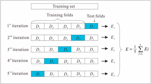
FIGURE 8. Sketch of K-fold cross-validation process.
5 Modeling process
A total of six modeling processes were performed to forecast the lithofacies types as follows: a) well logging data based on the SVM method in the point-to-point sample extraction mode; b) paleoenvironmental parameter data based on the SVM method in the point-to-point sample extraction mode; c) paleoenvironmental parameter data based on the SVM method in the curve shape-to-point sample extraction mode; d) well logging data based on the SVM method in the curve shape-to-point sample extraction mode; e) well logging data and paleoenvironmental parameter data based on the SVM method in the curve shape-to-point sample extraction mode; f) well logging data and paleoenvironmental parameter data based on the XGBoost method in the curve shape-to-point sample extraction mode.
The modeling flowchart of the lithofacies type forecasts based on the SVM and XGBoost models is shown in Figure 9. Each modeling process could be divided into three steps, namely, data preprocessing, model building, and model application.
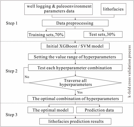
FIGURE 9. Modeling flowchart of lithofacies prediction based on support vector machine (SVM) and extreme gradient boosting (XGBoost) models.
Step 1. Data preprocessing: The lithofacies were numbered from 1 to 22: D1, 1; D2, 2; D3, 3; D4, 4; LL1, 5; LL2, 6; LL3, 7; LS1, 8; LS2, 9; LS3, 10; LS4, 11; MS1, 12; MS2, 13; MS3, 14; MS4, 15; SD1, 16; SD2, 17; SD3, 18; SD4, 19; US1, 20; US2, 21; and US3, 22. According to the different experimental conditions, a sample extraction mode was selected to extract samples from the raw data to build a correspondence sample dataset. Finally, the sample was randomly divided into training and prediction data at a ratio of 7:3, and the training data were further divided into five parts.
Step 2. Model building: The model was trained using the training data and K-fold cross-validation. The optimum model hyperparameters were selected. The SVM model had two important parameters, C and
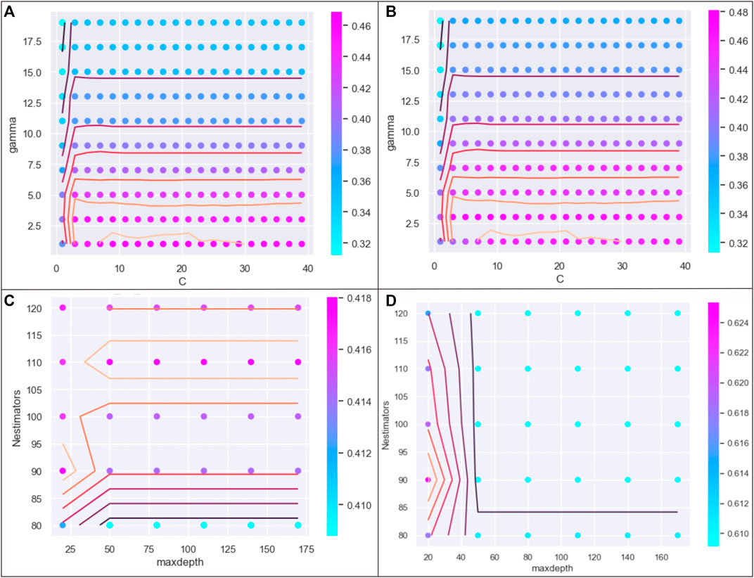
FIGURE 10. Cross-validation and parameter optimization analysis of models (a) and (f): (A) and (C) show the scores of forecast accuracies caulated by using training samples in model (a) and (f); (B) and (D) show the scores of forecast accuracies caulated by using testing samples in model (a) and (f).
Step 3. Model application: The optimal model was selected, and the lithofacies type forecasts were conducted to output the resulting map. Figure 10 also shows the complex relationship between the accuracy and the parameters. Overall, we observed no obvious linear relationship between them, and the accuracy was controlled by either the C and
6 Modeling results
The forecast accuracies of the six models were determined according to the output results, as shown in Figure 11 and Table 1. Model e) showed the highest average forecast accuracy for all lithofacies types, reaching 68%, as well as the highest average forecast accuracy for favorable lithofacies types at 98%. Model b) showed the lowest average forecast accuracy for all and favorable lithofacies types. Models d) and f) showed forecast accuracies similar to those of model e). Model c) showed a forecast accuracy similar to that of model b). Overall, model e) was the most applicable for the forecasting of lacustrine lithofacies types.
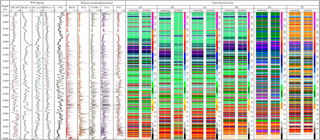
FIGURE 11. Shale lithofacies type modeling results at Well FY1 based on machine learning.
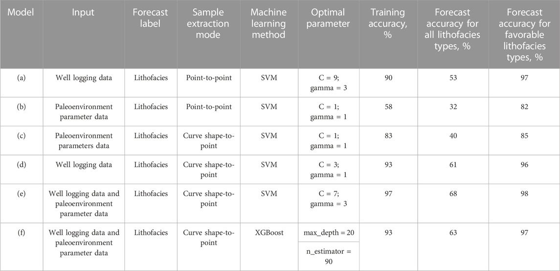
TABLE 1. Comparison of machine learning results for different modeling conditions.
For favorable lithofacies types, the average forecast accuracy of models (a-f) reached 82%–98%. The accuracy fully met the exploration requirements for accurately identifying target layers and confirmed the feasibility of machine learning for forecasting lacustrine lithofacies types. In addition, based on SVM, the average forecast accuracy of all lithofacies types was improved by 7%–28% using both well logging data and paleoenvironmental parameter data, rather than using just either data, and by 7%–8% by using the curve shape-to-point sample extraction mode compared to the point-to-point sample extraction mode. These improvements in forecast accuracy indicated that the introduction of paleoenvironmental parameters data was effective and that the sample extraction mode can affect the forecasting results. Therefore, when using machine learning to forecast lacustrine lithofacies types, the selection of data extraction mode and the application of data types are prerequisites for obtaining good results.
Overall, the modeling results reveal the forecast accuracies under different conditions (see Section 5), laying a foundation for finding effective methods and processes to forecast lacustrine shale lithofacies types in continental rift basins. When using machine learning methods, selecting the curved shape-to-point sample extraction mode and inputting both types of data is an effective way to improve the forecast accuracy.
7 Discussion
From a geological perspective, the relatively low average forecast accuracy for all lithofacies types occurred because the learning sample quantity of the different lithofacies types varied significantly. With many learning samples, the average forecast prediction accuracy is high, whereas the training accuracy is very low, leading to lower forecast accuracy. Figure 12 shows the relationship between the learning sample size and forecast accuracy. When the number of learning samples was >45 for a single lithofacies type, the forecast accuracy was >90%.
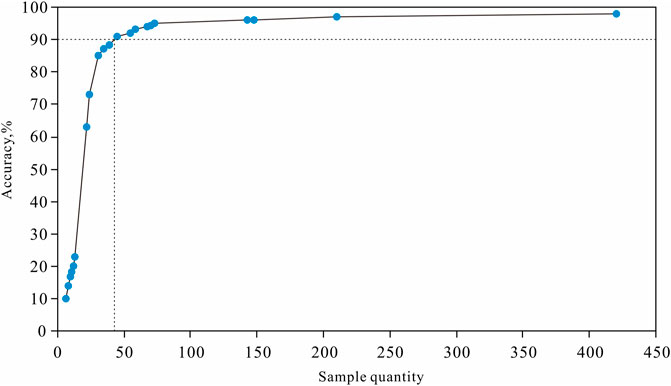
FIGURE 12. Relationship between learning sample quantity and forecast accuracy (statistics from model (a)).
Paleoenvironmental parameters directly influence shale lithofacies. Theoretically, the accuracy of lithofacies type forecasts using paleoenvironmental parameter data should be the highest; however, the actual forecast accuracy from the modeling results was quite low. The most likely explanation for this is the complex structure of lacustrine shale. For the same lithofacies tested by XRF at different locations, the paleoenvironmental parameters also differed due to heterogeneity within the lithofacies. In laminated lithofacies with limy and clayey lamina, the testing focal spot of XRF is in the lamina, producing different test results. This causes the value range of paleoenvironmental parameters to be relatively wide, overlapping with values in different lithofacies types, such as Sr content (Figure 13). This reduces the effectiveness of machine learning and the forecast accuracy, leading to a lower accuracy using paleoenvironmental parameter data.
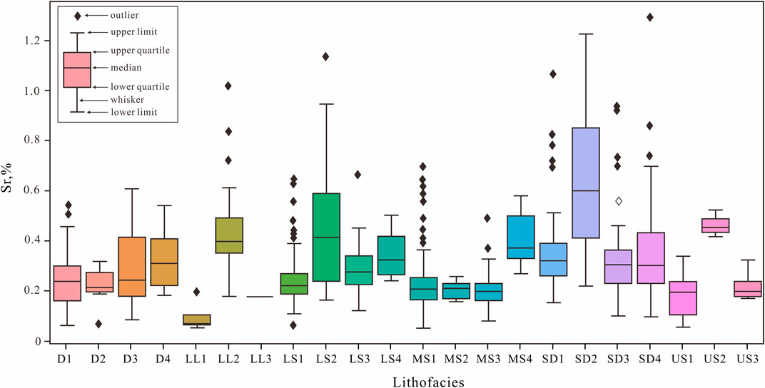
FIGURE 13. Boxplot of Sr content for different lithofacies types.
Machine learning is an effective method for solving complex geological problems. However, further research is required regarding lacustrine shale with strong heterogeneity in continental rift basins. First, rock microstructure is the key factor affecting shale reservoirs and is an important criterion for lithofacies classification, leading to heterogeneity and anisotropy in classification results. Therefore, additional physical experiments of rock microstructure are needed to further reveal the typical features of various lithofacies types and to enrich the learning samples. Second, correlation studies between logging response, element content or ratio, and shale microstructure are needed. Third, the current study did not improve on the calculation methods of SVM and XGBoost; thus, further optimization and improvement of machine learning methods are the focus of future research. We believe that the forecast accuracy of lacustrine shale lithofacies types can be improved by machine learning methods, which will be a positive step in the evaluation of shale oil sweet spots in oil fields worldwide.
8 Conclusion
The shale lithofacies in the upper Es4 unit of the Dongying Sag were distinguished using the components and structural changes shown in the core and thin sections. Considering the sedimentary composition and structure as the main criteria, the shale lithofacies of the upper Es4 unit in Dongying Sag were divided into six major and 22 minor types. Statistical analysis showed that the quantities and thicknesses of the different lithofacies types varied significantly.
Six machine learning-based modeling processes were conducted using well logging and paleoenvironmental parameter data. The forecast accuracy for all and favorable lithofacies types was highest when using both types of data to forecast lithofacies types using the SVM method and the curved shape-to-point sample extraction mode, whereas the accuracy was lowest when using only paleoenvironmental parameter data based on the SVM method with the point-to-point sample extraction mode.
The differences in the learning sample quantities of different lithofacies types affect the average forecast accuracy of all lithofacies types. The heterogeneity within the lithofacies results in a value range overlap with the paleoenvironmental parameter data, which also affects forecast accuracy.
Taken together, our results demonstrate progress compared to previous studies (i.e., Tahmasebi et al. (2017); Naeini and Prindle (2018); Dev and Eden (2019); Guo (2021)). First, we used a machine learning method to forecast the key features of the sedimentary structure of shales and lacustrine shale lithofacies type classification, rather than using these methods mainly to forecast mineral components, as in previous studies. Second, this study is the first to apply paleoenvironmental parameter data with well logging to forecast shale lithofacies types, which achieved significant forecast accuracy.
Data availability statement
The original contributions presented in the study are included in the article; further inquiries can be directed to the first author and corresponding authors.
Author contributions
All authors listed have made a substantial, direct, and intellectual contribution to the work and approved it for publication.
Funding
This study was financially supported by the National Science and Technology Major Project of China (No. 2017ZX05049-4), the Key Scientific and Technological Project of SINOPEC (KL21042), and the Key Scientific and Technological Research Project of Shengli Oilfield (YGK2204).
Conflict of interest
Authors ZF and SY were employed by the Research Institute of Petroleum Exploration and Development, Shengli Oilfield. Author ZF was employed by the Sinopec Key Laboratory of Shale Oil/Gas Exploration and Production, Shengli Oilfield Branch and by the Key Laboratory of Sedimentary Simulation and Reservoir Evaluation, Sinopec Shengli Oilfield.
The authors declare that this study received funding from SINOPEC and Shengli Oilfield Company. The funders were involved in the study design and collection of data, and not involved in analysis, interpretation of data, the writing of this article and the decision to submit it for publication.
Publisher’s note
All claims expressed in this article are solely those of the authors and do not necessarily represent those of their affiliated organizations, or those of the publisher, the editors, and the reviewers. Any product that may be evaluated in this article, or claim that may be made by its manufacturer, is not guaranteed or endorsed by the publisher.
References
Abouelresh, M., Babalola, L., Bokhari, A. K., Omer, M., and Kubur, A. (2020). Sedimentology, geochemistry and reservoir potential of the organic-rich qusaiba shale, tabuk basin, nw Saudi Arabia. Mar. Petroleum Geol. 111 (2020), 240–260. doi:10.1016/j.marpetgeo.2019.05.001
Ali, J., Ashraf, U., Anees, A., Peng, S., Umar, M. U., Thanh, H. V., et al. (2022). Hydrocarbon potential assessment of carbonate-bearing sediments in a meyal oil field, Pakistan: Insights from logging data using machine learning and quanti elan modeling. ACS Omega 7 (43), 39375–39395. doi:10.1021/acsomega.2c05759
Alkinani, H. H., Al-Hameedi, A. T., Dunn-Norman, S., Flori, R. E., Alsaba, M. T., and Amer, A. S. (2019). Applications of artificial neural networks in the petroleum industry: A review. In SPE Middle East oil and gas show and conference. doi:10.2118/195072-ms
Belyadi, F., and Fathi, E. (2021). New hybrid approach for developing automated machine learning workflows: A real case application in evaluation of marcellus shale gas production. Fuels 2 (3), 286–303. doi:10.3390/fuels2030017
Bergen, K. J., Johnson, P. A., de Hoop, M. V., and Beroza, G. C. (2019). Machine learning for data-driven discovery in solid Earth geoscience. Science 363 (6433), eaau0323. doi:10.1126/science.aau0323
Bhattacharya, S., and Carr, T. R. (2019). Integrated data-driven 3D shale lithofacies modeling of the Bakken Formation in the Williston basin, North Dakota, United States. J. Petroleum Sci. Eng. 177, 1072–1086. doi:10.1016/j.petrol.2019.02.036
Cao, B., Xuebin, D. U., Yongchao, L. U., Liu, H., Liu, Z., Yiquan, M. A., et al. (2019). Identification and controlling factors of multi-scale lithofacies for continental shale under an isochronous stratigraphic framework: A case study in dongying sag, bohai Bay Basin. Petroleum Geol. Exp. 41 (5), 752–761. doi:10.11781/sysydz201905752
Carey, C., Boucher, T., Mahadevan, S., Bartholomew, P., and Dyar., M. D. (2015). Machine learning tools for mineral recognition and classification from Raman spectroscopy. J. Raman Spectrosc. 46 (10), 894–903. doi:10.1002/jrs.4757
Chen, T., and Guestrin, C. (2016). XGBoost: A scalable tree boosting system. Proceedings of the 22nd ACM SIGKDD international conference on knowledge discovery and data mining. doi:10.1145/2939672.2939785
Dev, V. A., and Eden, M. R. (2019). Formation lithology classification using scalable gradient boosted decision trees. Comput. Chem. Eng. 128, 392–404. doi:10.1016/j.compchemeng.2019.06.001
Fu, J., Li, S., Xu, L., and Niu, X. (2018). Paleo-sedimentary environmental restoration and its significance of chang 7 member of triassic yanchang formation in ordos basin, NW China. Petroleum Explor. Dev. 45 (6), 998–1008. doi:10.1016/s1876-3804(18)30104-6
Guo, J. (2021). Research on lithology identification method based on mechanical specific energy principle and machine learning theory. Expert Syst. Appl. 189. doi:10.1016/j.eswa.2021.116142
Jia, C., Zou, C., Yang, Z., Zhu, R., and Jiang, L. (2018). Significant progress of continental petroleum geology theory in basins of central and Western China. Petroleum Explor. Dev. 45 (4), 546–560. doi:10.11698/PED.2018.04.02
Kalantari-Dahaghi, A., Mohaghegh, S., and Esmaili, S. (2015). Coupling numerical simulation and machine learning to model shale gas production at different time resolutions. J. Nat. Gas Sci. Eng. 25, 380–392. doi:10.1016/j.jngse.2015.04.018
Li, C., Shen, A., Chang, S., Liang, Z., Li, Z., and Meng, H. (2021). Application and contrast of machine learning in carbonate lithofacies log identification: A case study of longwangmiao formation of mx area in sichuan basin. Petroleum Reserv. Eval. Dev. 11 (4), 586–596. doi:10.13809/j.cnki.cn32-1825/te.2021.04.015
Li, M., Jin, Z., Dong, M., Ma, X., Li, Z., Jiang, Q., et al. (2020). Design study of a dedicated head and neck cancer PET system. Petroleum Geol. Exp. 42 (4), 489–497. doi:10.1109/trpms.2020.2964293
Li, M., Ma, X., Jiang, Q., Li, Z., Pang, X., and Zhang, C. (2019). Enlightenment from formation conditions and enrichment characteristics of marine shale oil in North America. Petroleum Geol. Recovery Effic. 26 (1), 13–28. doi:10.13673/j.cnki.cn37-1359/te.2019.01.002
Li, Z., Liu, Y., Zhang, L., Zhao, H., Chen, X., and Wu, H. (2019). Application of data mining method in lithology identification using well log. Fault-Block Oil Gas Field 26 (6), 713–718. doi:10.6056/dkyqt201906007
Li, Z., LiZhang, L., Yuan, W., Chen, X., Zhang, L., and Li, M. (2022). Logging identification for diagenetic facies of tight sandstone reservoirs: A case study in the lower jurassic ahe formation, kuqa depression of tarim basin. Mar. Petroleum Geol. 139, 105601. doi:10.1016/j.marpetgeo.2022.105601
Liang, C., Jiang, Z., Cao, Y., Wu, J., Wang, Y., and Hao, F. (2017). Sedimentary characteristics and origin of lacustrine organic-rich shales in the salinized Eocene Dongying Depression. Geol. Soc. Am. Bull. 130 (1-2), 154–174. doi:10.1130/B31584.1
Liang, C., Jiang, Z., Cao, Y., Wu, M., Guo, L., and Zhang, C. (2016). Deep-water depositional mechanisms and significance for unconventional hydrocarbon exploration: A case study from the lower silurian longmaxi shale in the southeastern sichuan basin. AAPG Bull. 100 (5), 773–794. doi:10.1306/02031615002
Liu, J., Wang, J., Cao, Y. C., and Song, G. (2017). Sedimentation in a continental high-frequency oscillatory lake in an arid climatic background: A case study of the lower eocene in the dongying depression, China. J. Earth Sci. 28 (4), 628–644. doi:10.1007/s12583-016-0635-2
Liu, S., Cao, Y., and Liang, C. (2019). Lithologic characteristics and sedimentary environment of fine-grained sedimentary rocks of the Paleogene in Dongying sag, Bohai Bay Basin. J. Palaeogeogr. 21 (3), 479–489. doi:10.7605/gdlxb.2019.03.030
Liu, X., Tian, Z., and Chen, C.(2021). Total organic carbon content prediction in lacustrine shale using extreme gradient boosting machine learning based on bayesian optimization. Geofluids 2021, 1–18. doi:10.1155/2021/6155663
LoucksRuppel, R. G. S. C. (2007). Mississippian barnett shale: Lithofacies and depositional setting of a deep-water shale-gas succession in the fort worth basin, Texas. AAPG Bull. 91 (4), 579–601. doi:10.1306/11020606059
Naeini, E. Z., and Prindle, K. (2018). Machine learning and learning from machines. Lead. Edge 37 (12), 886–893. doi:10.1190/tle37120886.1
Niu, Y., Hu, Y., and Wang, J. (2023). Cracking characteristics and damage assessment of filled rocks using acoustic emission technology. Int. J. Geomechanics 23 (4). doi:10.1061/IJGNAI.GMENG-8034
Rothwell, R. G., and Croudace, I. W. (2015). “Micro-XRF studies of sediment cores: A perspective on capability and application in the environmental sciences,” in Micro-XRF studies of sediment cores, 1–21. doi:10.1007/978-94-017-9849-5_1
Shi, X., Wang, J., Liu, G., Yang, L., Ge, X., and Jiang, S. (2016). Application of extreme learning machine and neural networks in total organic carbon content prediction in organic shale with wire line logs. J. Nat. Gas Sci. Eng. 33, 687–702. doi:10.1016/j.jngse.2016.05.060
Song, M., Kim, S. H., Ryoo, G. H., Kim, M. K., Cha, H. N., Park, S. Y., et al. (2019). Adipose sirtuin 6 drives macrophage polarization toward M2 through IL-4 production and maintains systemic insulin sensitivity in mice and humans. Petroleum Geol. Recovery Effic. 26 (1), 1–10. doi:10.1038/s12276-019-0256-9
Suykens, J. A. K., and Vandewalle, J. (1999). Least squares support vector machine classifier. Neural Process. Lett. 9 (3), 293–300. doi:10.1023/a:1018628609742
Tahmasebi, P., Javadpour, F., and Sahimi, M. (2017). Data mining and machine learning for identifying sweet spots in shale reservoirs. Expert Syst. Appl. 88, 435–447. doi:10.1016/j.eswa.2017.07.015
Tian, J., Xin, X., Ma, W., Jin, H., and Wang, P. (2011). X-ray fluorescence core scanning records of chemical weathering and monsoon evolution over the past 5 Myr in the southern South China Sea. Paleoceanography 26 (4), 1–17. doi:10.1029/2010PA002045
Vapnik, V. N. (1999). An overview of statistical learning theory. IEEE Trans. Neural Netw. 10 (5), 988–999. doi:10.1109/72.788640
Wang, T., Zhu, X., Dong, Y., Yang, D., S, Bin., Tan, M., et al. (2021). Signals of depositional response to the deep time paleoclimate in continental depression lakes: Insight from the Anjihaihe Formation in the northwestern Junggar Basin. Earth Sci. Front. 28 (1), 60–76. doi:10.13745/j.esf.sf.2020.5.8
Wang, Y., Liu, H., Song, G., Xiong, W., Zhu, D., Zhu, D., et al. (2019). TMT-based quantitative proteomics revealed follicle-stimulating hormone (FSH)-related molecular characterizations for potentially prognostic assessment and personalized treatment of FSH-positive non-functional pituitary adenomas. Acta Pet. Sin. 40 (4), 395–414. doi:10.1007/s13167-019-00187-w
Wang, Y., Wang, X., Song, G., Liu, H., Zhu, D., Ding, J., et al. (2016). Genetic connection between mud shale lithofacies and shale oil enrichment in Jiyang Depression, Bohai Bay Basin. Petroleum Explor. Dev. 43 (5), 759–768. doi:10.1016/S1876-3804(16)30091-X
Yang, H., Zhao, Y., Cui, Q., Ren, W., and Li, Q. (2021).Paleoclimatic indication of X-ray fluorescence core-scanned Rb/Sr ratios: A case study in the zoige basin in the eastern Tibetan plateau. Sci. China Earth Sci. 51(1): 80–95. doi:10.1007/s11430-020-9667-7
Zhang, L., Li, J., Wang, W., Li, C., Zhang, Y., Jiang, S., et al. (2022). Diagenetic facies characteristics and quantitative prediction via wireline logs based on machine learning: A case of lianggaoshan tight sandstone, fuling area, southeastern sichuan basin, southwest China. Front. Earth Sci. 10. doi:10.3389/feart.2022.1018442
Zhang, S., Liu, H., Liu, Y., Wang, Y., Wang, M., Bao, Y., et al. (2020). Main controls and geological sweet spot types in Paleogene shale oil rich areas of the Jiyang Depression, Bohai Bay basin, China. Mar. Petroleum Geol. 111, 576–587. doi:10.1016/j.marpetgeo.2019.08.054
Zhou, K., Zhang, J., Ren, Y., Huang, Z., and Zhao, L. (2020). A gradient boosting decision tree algorithm combining synthetic minority over-sampling technique for lithology identification. Geophysics 85, WA147–WA158. doi:10.1190/geo2019-0429.1
Keywords: continental rift basin, lacustrine shale, lithofacies classification, machine learning, lithofacies types forecast
Citation: Fang Z, Zhang L and Yan S (2023) Forecast of lacustrine shale lithofacies types in continental rift basins based on machine learning: A case study from Dongying Sag, Jiyang Depression, Bohai Bay Basin, China. Front. Earth Sci. 11:1047981. doi: 10.3389/feart.2023.1047981
Received: 19 September 2022; Accepted: 04 April 2023;
Published: 20 April 2023.
Edited by:
Sid-Ali Ouadfeul, Sonatrach, AlgeriaReviewed by:
Chenyang Bai, China University of Geosciences, ChinaYong Niu, Shaoxing University, China
Nan Xiao, Changsha University of Science and Technology, China
Wanju Yuan, Geological Survey of Canada, Canada
Copyright © 2023 Fang, Zhang and Yan. This is an open-access article distributed under the terms of the Creative Commons Attribution License (CC BY). The use, distribution or reproduction in other forums is permitted, provided the original author(s) and the copyright owner(s) are credited and that the original publication in this journal is cited, in accordance with accepted academic practice. No use, distribution or reproduction is permitted which does not comply with these terms.
*Correspondence: Liqiang Zhang, emhhbmdscUB1cGMuZWR1LmNu