Intelligent velocity picking considering an expert experience based on the Chan–Vese model and mean-shift clustering

The velocity of seismic data can initially be established by identifying energy clusters on velocity spectra at different moments, which is crucial to the migration imaging and the stacking of common midpoint (CMP) gathers in the seismic data processing. However, the identification of energy clusters currently relies on manual work, with low efficiency and different standards. With the increasing application of wide-frequency, wide-azimuth, and high-density seismic exploration technology, the amount of seismic data has increased significantly, greatly increasing the cost of manual labor and time. In this paper, an intelligent velocity picking method based on the Chan–Vese (CV) model and mean-shift clustering algorithm was proposed. It can be divided into three steps. First, a velocity trend band is set up on the velocity spectrum by experts to avoid multiples and other noises. Then, the velocity trend band is applied to the Chan–Vese model as the initial time condition to segment the velocity spectrum and obtain the velocity candidate region. Finally, mean-shift clustering is adopted to cluster the useful energy clusters retained in the candidate region derived from the Chan–Vese model. When implementing the mean-shift clustering algorithm, the Gaussian kernel function and the energy of the velocity spectrum are utilized to control the efficiency and accuracy of the cluster. The tests of the model and real data prove that the proposed method can dramatically improve the accuracy and efficiency of velocity picking compared with the K-means and manual picking method.

1 Introduction

Velocity analysis of a seismic wave is a critical step in seismic data processing and also the basis for subsequent data processing procedures and interpretation. For example, the normal moveout (NMO) correction relies on stacking velocity (Wang et al., 2021a), the migration imaging relies on migration velocity (Jones et al., 1998; Nemeth et al., 1999; Hou & Marfurt, 2002), and time–depth conversion relies on time-domain velocity (Cameron et al., 2008). If the velocity field is accurate, the seismic profiles obtained by migration can reflect the underground structure more clearly. Currently, the velocity is mainly obtained by manually picking the velocity energy clusters. Although manual picking makes full use of expert experience, it is labor-intensive and repetitive. Moreover, the manual way is generally of low density in the picking of a velocity spectrum and has different views on the characterization of complex geological structures. Therefore, it is imperative to establish an efficient automatic velocity picking method to relieve the labor and improve the accuracy of velocity imaging in structures, following the main principle of the manual method and making full use of expert knowledge, especially with the increase in seismic data.

In order to improve efficiency and accuracy, in the early days, model-driven automatic velocity picking algorithms were developed rapidly. From the fundamentals, considering the mathematical and physical relationship between velocity and seismic data is the main thought behind these model-driven algorithms. A large number of scholars used an iterative optimization method to search for the optimal velocity by establishing an objective function that could represent waveform consistency or stacked energy. Toldi (1989) was the first to suggest the automatic velocity picking method. He designed an objective function by maximizing the sum of stacked energy, and the optimal velocity is obtained by iterative updating. However, this method assumes that the model is linear but not in practice, and this brings about inapplicability in low signal-to-noise seismic data. Moreover, this method considers a lot of constraints and complicates the model, which makes the practical performance of the method very poor. Zhang et al. (2015) established a non-linear objective function by analyzing the selected velocity distribution rules, which can achieve automatic velocity picking; however, this still does not solve the large computational effort and low noise immunity of the model-driven approach. Moreover, Wilson and Gross (2019) used a particle swarm optimization method to find the optimal time difference to flatten the hyperbolic curve which solves the local minimum problems partially. Velis (2021) gave a non-hyperbolic and anisotropic velocity analysis algorithm. The objective function of non-hyperbolic energy involved the anisotropy parameters, and the velocity was established by the simulated annealing-based iterative search. In this method, static and dynamic boundaries were used to avoid multiple noises. In addition, Yuan et al. (2019) proposed that full waveform inversion can also retrieve the background velocity structure, and the low-frequency full-waveform inversion result was considered as an a priori model, which can be applied to reservoir prediction. However, the full waveform inversion is a strong non-linear inversion. When the accuracy of the initial velocity model is not enough, there will be cycle jumps and it will result in failure. All in all, the model-driven method requires the hypothesis that the mathematical physical model used can accurately express the relationship between seismic data and velocity, causing the problems of local minima and large costs of computation.

In recent years, due to the significant improvement in computer performance, machine learning has been applied to various fields, such as tumor and liver segmentation in CT images (Aghamohammadi et al., 2021), brain tumor segmentation (Ranjbarzadeh et al., 2021), and breast tumor segmentation in mammograms (Ranjbarzadeh et al., 2022). Also, for geophysics, underground structure segmentation, automatic velocity picking can be achieved by deep learning methods or unsupervised clustering methods.

Compared to traditional model-driven methods, deep learning can be regarded as a data-driven method, which can establish an optimal non-linear mapping relationship between seismic data (e.g., common middle point gathers, velocity spectra, or shot gathers) and velocity. The deep learning method updates the network parameters mainly through a certain depth of neural network model and a back-propagation algorithm (Rumelhart et al., 1986), as well as automatically learning the effective features in data and the establishment of multi-domain mapping (LeCun et al., 2015; Goodfellow et al., 2016). Park and Sacchi (2020) proposed the velocity automatic picking method based on the convolutional neural network (CNN); this class of methods transforms the identification of energy clusters on a velocity spectrum into a classification problem in the field of image recognition; hence, this method requires a high signal-to-noise ratio of the velocity spectrum. Biswas et al. (2019) and Zhang et al. (2019) proposed the recurrent neural network (RNN)-based automatic velocity picking method, which considers the temporal order of seismic data and treats the velocity picking as a normalization problem, resulting in higher accuracy. In addition, Fabien-Ouellet and Sarkar (2020) combined the CNN and long- and short-term memory (LSTM) network to estimate the root mean square velocity and interval velocity of seismic data. The combination of these two networks can simultaneously learn the characteristics of CMP gathers and velocity spectra to more accurately predict the velocity. Wang et al. (2020) contrasted the velocity picking algorithms of the regression-based neural network and the classification-based neural network and claimed that both methods could reasonably predict the velocity field. Then, Yuan et al. (2022) proposed a double-scale gated recurrent unit neural network method, which uses data-driven methods to learn forward, and inversion simulations to establish the non-linear relationship between post-stack data and velocity or impedance; this method recovers the low-frequency impedance so as to make the velocity field more accurate, and geological laws and blind wells can verify its rationality. Recently, Cao et al. (2022) proposed a seismic velocity inversion method based on the CNN-LSTM fusion deep neural network, which can simultaneously estimate the root mean square velocity and interval velocity from the CMP gather. In the proposed method, a CNN encoder and two LSTMs are used to extract spatial and temporal features from seismic data, and a CNN decoder is used to recover the velocity, improving the accuracy of imaging. As a whole, all the deep learning methods mentioned above that get rid of the ill-posed inverse problem of the traditional model-driven method use artificial neural networks to establish a non-linear mapping relationship between seismic data or a velocity spectrum (input) and a velocity model (output). However, such supervised neural network intelligent velocity picking methods require professionals to manually pick up a rich and large amount of labeled data for training, which is time-consuming and has weak generalization ability. When predicting seismic data with different features, the labeled data need to be reconstructed with a retrained network. In addition, it is impossible to interpret the process of training since the prediction process of seismic data is a huge composite function.

For the attractive unsupervised clustering method, it can search for energy cluster features of velocity without constantly establishing labels and training according to different data. This type of intelligent picking method groups the energy clusters of velocity with the same features used to obtain the approximate distribution of the data. It has a simple algorithm and is easy to implement. In addition, it is highly interpretable and generalizable, adapting to seismic data of any features. Therefore, it is more extensible in industrial applications. Agudelo et al. (2017) and Araya-Polo et al. (2017) use the K-means clustering algorithm that uses the distance of samples as a similarity indicator to process the seismic data, and the class center is regarded as the picking location. However, it poorly clusters non-spherical energy clusters of velocity, and the K values need to be fixed manually. Chen et al. (2018) proposed a bottom-up strategy, considering the problem of different K values for different velocity spectra, which solves the drawback of fixed K values to some extent. Waheed et al. (2019) also applied the density clustering method to pick up the energy clusters of velocity to achieve automatic velocity picking, which avoids the problem of choosing K values manually in K-means clustering. In addition, Wang et al. (2021b) proposed an approach based on adaptive threshold-constrained K-means; this method can improve the identification of the energy cluster of velocity which was weak on the velocity spectrum. Wang et al. (2022) also suggested a Gaussian mixture clustering method to achieve automatic velocity picking, as an extreme case of the Gaussian mixture model, and K-means is difficult to characterize velocity energy clusters with low focus ability, while the Gaussian mixture model can accurately fit and provide uncertainty analysis at the same time. These unsupervised clustering algorithms, however, only consider the ability to identify energy clusters of the velocity, without taking into account the complexity of the actual seismic data and expert experiences, resulting in the velocity picking methods affected by the multiples and some other noises on the velocity spectrum.

In this article, we proposed an automatic velocity picking method based on the Chan–Vese (CV) model and mean-shift clustering algorithm, which can effectively improve the accuracy and efficiency of velocity picking and solve the interference of multiples. Meanwhile, the method we proposed can also reduce the manual labor and improve the adaptability of unsupervised clustering methods in actual seismic data. First, a velocity trend band is set up on the velocity spectrum by experts to avoid multiples and noises. Then, the velocity trend band is applied to the CV model as the initial time condition to segment the valid energy clusters of velocity on the velocity spectrum. Finally, the mean-shift clustering algorithm is adopted to cluster the valid energy clusters in the candidate region derived from the CV model. In order to improve the accuracy and efficiency of mean-shift clustering, the Gaussian kernel function and the energy value of velocity are applied for weighting, which allows the identification of not only the isolated and highly focused energy clusters of velocity but also the interconnected energy clusters.

2 Methods

We started with a brief analysis of how seismic data processors perform velocity picking. After obtaining a CMP velocity spectrum, the processor first analyzes the trend and range of velocity for that CMP using empirical and geological knowledge; then, the energy clusters of effective reflected waves within the correct trend are identified with the naked eye and cluster centers are picked up as the velocity for that location. The entire picking is the process by which processors translate geophysical and geological theories into the geometry of energy clusters on the velocity spectrum (Wang et al., 2022). Our method follows this process to achieve automatic velocity picking. Corresponding to the first step of manual picking, the valid velocity trend and range are identified using the CV model with expert experience constraints, and the second step of manual picking is replaced by the mean-shift clustering method.

The main body of our method in this article can be divided into three parts, as shown in Figure 1. The first step is the pre-processing of the velocity spectrum, including the size regularization of the velocity spectrum and the random noise filtering. The size regularization of the velocity spectrum is to make the time dimension of each velocity spectrum consistent so as to ensure that the velocity curve picked up in every velocity spectrum, subsequently, has the same sampling time for stacking; generally, this time dimension is consistent with the seismic records. Random noise filtering is used to filter some salt-and-pepper noises on the velocity spectrum by using the median filtering method so as to improve the accuracy of energy cluster identification of the subsequent CV model. The second step is the output of the effective candidate region of velocity by the CV model, the expert experience constraints, and the grayscale based on velocity spectrum energy, which is the normalization of velocity spectrum energy that is performed in this step. The third step is the use of the mean-shift clustering method to pick up the centers of the effective reflected energy clusters, and the Gaussian kernel function and energy weighting constraints are applied in this step. These steps are discussed in the following sections in detail.

FIGURE 1

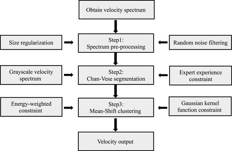
FIGURE 1. Intelligent velocity picking workflow.

2.1 CV model in velocity spectrum segmentation

Image segmentation is an important image analysis and processing technology that has been widely used in medical image analysis, intelligent traffic management, remote sensing image processing, and other fields (Li et al., 2021). Image segmentation methods include threshold segmentation, region segmentation, edge segmentation, and the active contour model and level set methods (Osher & Sethian, 1988). Getreuer (2012) shows that based on level set methods, Chan and Vese proposed the CV model which solves the problem of computational difficulty caused by the primary length term and the secondary area term in the expression. Keegan et al. (2017) proposed that the CV model be the basis of multi-phase image segmentation, and the model does not need to define the boundary by gradient, which significantly reduces the complexity and improves the efficiency of segmentation.

2.1.1 Theory of the CV model

The differences in location, size, and shape of velocity spectrum energy clusters make the level-set-based CV model more effective. The energy function of the CV model can be expressed as follows:

$E\left(C\right)=\mu \mathit{L}\mathit{e}\mathit{n}\mathit{g}\mathit{t}\mathit{h}\left(C\right)+\upsilon \mathit{A}\mathit{r}\mathit{e}\mathit{a}\left(C\right)+{\lambda }_1{E}_1\left(C\right)+{\lambda }_2{E}_2\left(C\right),(1)$

where the first term of $E\left(C\right)$ is the length constraint of the evolution curve, in which the curve (C) is originally provided by an effective velocity trend band on the velocity spectrum; the second term is the shape constraint of C; and the third and fourth terms are the pixel losses based on the grayscale map of the velocity spectrum inside and outside C, respectively, which are calculated by Eqs 2, 3. $\mu$, $\upsilon$, ${\lambda }_1$, and ${\lambda }_2$ are the constant coefficients, which are generally taken as 1.

$E_1\left(C\right)={\underset{\mathrm{i}\mathrm{n}\mathrm{s}\mathrm{i}\mathrm{d}\mathrm{e}\left(C\right)}{{\displaystyle \int }}\left|I_0\left(x,y\right)-C_1\right|}^{2}dxdy,(2)$

$E_2\left(C\right)={\underset{\mathrm{o}\mathrm{u}\mathrm{t}\mathrm{s}\mathrm{i}\mathrm{d}\mathrm{e}\left(C\right)}{{\displaystyle \int }}\left|I_0\left(x,y\right)-C_2\right|}^{2}dxdy,(3)$

where $I_0\left(x,y\right)$ denotes each pixel value of the inner region and outer region of the evolution curve C. $C_1$ and $C_2$ are the average of the pixels in the inner and outer regions of curve C, respectively. $E_1\left(C\right)$ and $E_2\left(C\right)$ are minimized when the evolution curve C can correctly partition the effective reflected energy clusters of the velocity spectrum.

To correctly solve the evolution of C, the CV model uses the level set method when the energy function is minimized, and the level set method replaces the evolution of C with the evolution of a curved surface $\varphi \left(x,y\right)$. The specific programs are as follows:

$\left\{\begin{array}{l}C=\partial \omega =\left\{\left(x,y\right)\in \mathrm{\Omega }:\varphi \left(x,y\right)=0\right\}\\ \mathit{i}\mathit{n}\mathit{s}\mathit{i}\mathit{d}\mathit{e}\left(C\right)=\omega =\left\{\left(x,y\right)\in \mathrm{\Omega }:\varphi \left(x,y\right)>0\right\}\\ \mathit{o}\mathit{u}\mathit{t}\mathit{s}\mathit{i}\mathit{d}\mathit{e}\left(C\right)=\mathrm{\Omega }\backslash \overline{\omega }=\left\{\left(x,y\right)\in \mathrm{\Omega }:\varphi \left(x,y\right)<0\right\}\end{array}\right..(4)$

C is denoted by $\varphi \left(x,y\right)=0$. The inner region of C is denoted by $\varphi \left(x,y\right)>0$, and the outer region of C is denoted by $\varphi \left(x,y\right)<0$. Then, we define a step function and its derivative as

$H\left(z\right)=\left\{\begin{array}{cc}1,& z>0,\\ 0,& z<0,\end{array}\right.(5)$

${\delta }_0\left(z\right)=\frac{d}{dz}H\left(z\right).(6)$

Substituting Eqs 4–6 into Eq 1, the energy function of the curved surface based on the level set is obtained as follows:

$\begin{array}{l}E(\varphi (x,y))=\mu \underset{\mathrm{\Omega }}{{\displaystyle \int }}\left|\nabla H\left(\varphi \left(x,y\right)\right)\right|dxdy+\nu \underset{\mathrm{\Omega }}{{\displaystyle \int }}\left.H(\varphi (x,y\right))dxdy\\ +{\lambda }_1{\underset{\mathrm{\Omega }}{{\displaystyle \int }}\left|I_0\left(x,y\right)-C_1\right|}^{2}H\left(\varphi \left(x,y\right)\right)dxdy\\ +{\lambda }_2{\underset{\mathrm{\Omega }}{{\displaystyle \int }}\left|I_0\left(x,y\right)-C_2\right|}^2(1-H(\varphi (x,y))dxdy\end{array}.(7)$

Using the energy function $E$ and its corresponding Euler–Lagrange to minimize Eq 7, the result is

$\frac{\partial \varphi }{\partial t}={\delta }_0\left(\varphi \right)\left[\mu \mathit{div}\left(\frac{\nabla \varphi }{\left|\nabla \varphi \right|}\right)-\nu -{\lambda }_1{\left(I-C_1\right)}^2+{\lambda }_2{\left(I-C_2\right)}^2\right],(8)$

$C_1=\frac{\underset{\mathrm{\Omega }}{{\displaystyle \int }}{I}_0\left(x,y\right)H\left(\varphi \left(x,y\right)\right)dxdy}{\underset{\mathrm{\Omega }}{{\displaystyle \int }}H\left(\varphi \left(x,y\right)\right)dxdy},(9)$

$C_2=\frac{\underset{\mathrm{\Omega }}{{\displaystyle \int }}{I}_0(x,y)(1-H(\varphi (x,y))dxdy}{\underset{\mathrm{\Omega }}{{\displaystyle \int }}\left(1-H(\varphi (x,y))dxdy\right.}.(10)$

Therefore, the final evolution partial differential equation of the CV model is

$\left\{\begin{array}{l}\frac{\partial \varphi }{\partial t}={\delta }_0\left(\varphi \right)\left[\mu \mathit{div}\left(\frac{\nabla \varphi }{\left|\nabla \varphi \right|}\right)-\nu -{\lambda }_1{\left(I-C_1\right)}^2+{\lambda }_2{\left(I-C_2\right)}^2\right]\\ \varphi {|}_{t=0}=u\left(x,y\right)\end{array}\right.,(11)$

where $u\left(x,y\right)$ denotes C at the initial moment of the evolution equation. In our method, to obtain faster and more accurate segmentation results, experts are required to combine geophysical and geological theories to give the original range of velocity, which is treated as $u\left(x,y\right)$, and the energy clusters outside the $u\left(x,y\right)$ are not involved in the subsequent clustering. Then, the following advantages can be obtained:

1) The curve evolution speed can be accelerated

2) The interference of multiples and other noises can be avoided

3) The valid velocity candidate region can be provided for mean-shift clustering

Also, the process of segmenting the velocity spectrum using the CV model can be summarized as follows:

1) Size regularization and random noise filtering for the velocity spectrum

2) Energy-oriented grayscale of the velocity spectrum

3) Provide an initial evolutionary curve by experts

4) Evolve segmentation curves to obtain an effective velocity candidate region for mean-shift clustering

2.1.2 Velocity spectrum segmentation examples

Our aim is that the CV model can segment the velocity energy clusters that are truly effective as shown in Figure 2 and Figure 3, just as the manual pickup of energy clusters. We applied the CV model with expert constraints previously to the velocity spectra of one synthetic data and one real data. Depending on the lateral variation of the velocity, the expert constraint bands were implemented at intervals of 10 and 500 velocity spectra. Figure 2 shows the segmentation result of the 40th velocity spectrum of the Marmuosi model (Martin et al., 2006). For high signal-to-noise ratio synthetic data, the CV model can well identify the effective energy clusters of the velocity. Figure 3 shows the segmentation results of the 3900th velocity spectrum of the real data, which develops multiples in 6–9 s. The energy clusters of multiples velocity are interference signals, which generally appear in the high-time low-velocity region in the velocity spectrum as shown in Figure 3, and the CV model can avoid the effect of multiples energy clusters after the expert experience constraint and just obtaining the valid energy clusters of the velocity.

FIGURE 2

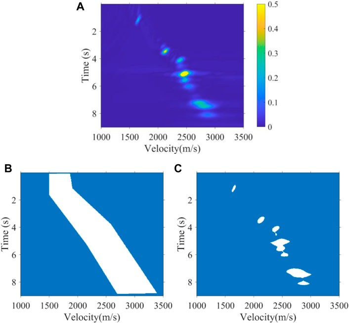
FIGURE 2. (A) 40th velocity spectrum with a high signal-to-noise ratio of the Marmuosi model, (B) expert experience constraint band, and (C) segmentation result.

FIGURE 3

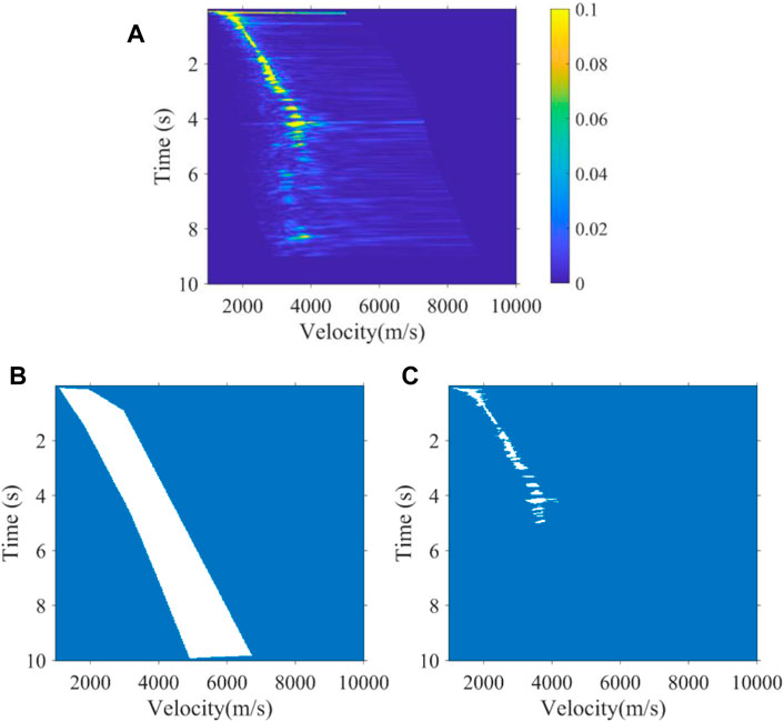
FIGURE 3. (A) 3900th velocity spectrum with multiple developments in 6–9 s of real data, (B) expert experience constraint band, and (C) segmentation result.

2.2 Mean-shift clustering for energy cluster picking

Mean-shift clustering based on density does not need to artificially determine the number of clusters and the initial cluster center locations like other algorithms, such as K-means. It can automatically select the number of clusters based on the density distribution of the data (Wang et al., 2018). Therefore, mean-shift clustering can be well adapted to a case of a continuous distribution of energy clusters on the velocity spectrum. At the same time, mean-shift clustering is less computational, faster, and more stable, so we use mean-shift clustering to improve efficiency.

2.2.1 Theory of mean-shift clustering

The mean-shift algorithm (Comaniciu and Meer, 2002) is an iterative process in which the mean value position of the energy cluster is calculated. In each iteration, the mean value position is updated and then the updated position is used as a new start to calculate the shift value until it reaches the threshold. The calculation of the shift value can be expressed as

${\mathbf{M}}_h=\frac{1}{k}{\displaystyle \sum }_{{\mathbf{x}}_i\in D_h}\left({\mathbf{x}}_i-\mathbf{x}\right),(12)$

where $\mathbf{x}$ is the mean value position of the circle $D_h$ with $\mathbf{x}$ as the center and $h$ as the radius, and ${\mathbf{x}}_i$ is the position of every energy point within $D_h$. $k$ is the number of energy points within $D_h$. Then, the $\mathbf{x}$ is updated by

${\mathbf{x}}^{*}=\mathbf{x}+{\mathbf{M}}_h.(13)$

Eqs 12, 13 allow the mean value position to continuously move toward the center of energy clusters, and the update stops when the shift value ${\mathbf{M}}_h$ is less than the threshold value.

As shown in Eq. 12, the contribution of energy points within $D_h$ are the same when calculating the shift value; however, the energy of each point on the velocity spectrum is different, leading to different contributions. The larger the energy, the more the contributions will be. Therefore, we applied an improved calculation of the shift value based on energy weighting to improve the accuracy of energy cluster picking:

${\mathbf{M}}_h=\frac{{\sum }_{i=1}^{n}G\left({‖\frac{{\mathbf{x}}_i-\mathbf{x}}{h}‖}^2\right)\omega \left({\mathbf{x}}_i\right)\left({\mathbf{x}}_i-\mathbf{x}\right)}{{\sum }_{i=1}^{n}G\left({‖\frac{{\mathbf{x}}_i-\mathbf{x}}{h}‖}^2\right)\omega \left({\mathbf{x}}_i\right)},(14)$

where $G$ is the Gaussian kernel function, $h$ denotes the radius of the region $D_h$, and $\omega \left({\mathbf{x}}_i\right)$ is the energy of ${\mathbf{x}}_i$ within the region $D_h$. Substituting Eq. 14 into Eq. 13 to obtain the new update equation, we get

${\mathbf{x}}^{*}=\frac{{\sum }_{i=1}^{n}G\left({‖\frac{{\mathbf{x}}_i-\mathbf{x}}{h}‖}^2\right)\omega \left({\mathbf{x}}_i\right){\mathbf{x}}_i}{{\sum }_{i=1}^{n}G\left({‖\frac{{\mathbf{x}}_i-\mathbf{x}}{h}‖}^2\right)\omega \left({\mathbf{x}}_i\right)}.(15)$

Eq. 15 is used to iterate the mean value position of the energy cluster, until ${\mathbf{x}}^{*}$ moves to the position where the energy of the cluster is maximum, which is regarded as the picking position.

2.2.2 Examples of velocity picking using mean-shift clustering

We applied the mean-shift clustering method proposed previously to identify the segmentation results of the CV model in subsection 2.2. Due to the constraints of expert experience, the CV model only selects the valid energy clusters of the velocity of effective reflection seismic waves and abandons the incorrect energy clusters of the velocity of disturbing multiples in deep regions. In fact, the most classic manual method is based on personal experience to roughly pick up the valid velocity energy clusters, while there is no valid energy cluster in the deep region of a velocity spectrum, and they obtain the velocity by using velocity curve fitting. So, when using the mean-shift clustering method, only the energy clusters segmented by the CV model several times are picked up. At other sampling times without valid energy clusters, we obtain the velocity by fitting the velocity curve according to the expert experience trend and accurate velocity obtained intelligently. To illustrate the correctness of our proposed method more intuitively, we place the real velocity of the Marmousi model and most classic manual picking results of real data in Figure 4 and Figure 5 for comparison, respectively. Furthermore, Figure 4 shows the picking results of the 40th velocity spectrum of the Marmuosi model, and Figure 5 shows the picking results of the 3900th velocity spectrum of the real data. These tests show whether the velocity spectrum has a high signal-to-noise ratio or interfering multiples development, and the intelligent picking results we proposed in this article always conform to the manual picking result; this means that our automatic picking method can replace manual picking for high accuracy and efficiency, with each velocity spectrum being picked up in just 1 s.

FIGURE 4

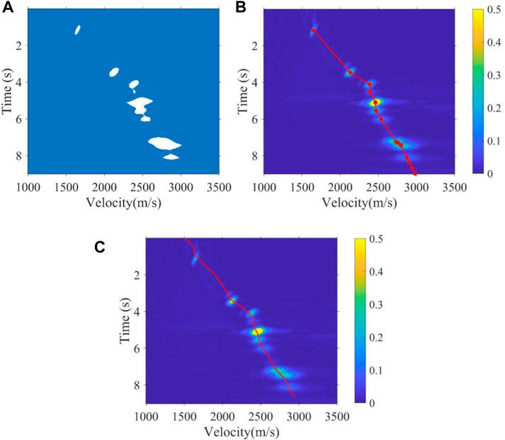
FIGURE 4. 40th velocity spectrum of the Marmuosi model. (A) Segmentation result, (B) intelligent picking result by using the method proposed, and (C) real velocity curve.

FIGURE 5

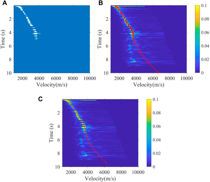
FIGURE 5. 3900th velocity spectrum with multiple developments in 6–9 s of real data. (A) Segmentation result, (B) intelligent picking result by using the method proposed, and (C) manual picking result by semblance analysis.

3 Examples

3.1 Synthetic data

To test the feasibility of the proposed method, we tested the 2D Marmousi model shown in Figure 6A with 60 velocity spectra responding to 60 CMPs, while the distribution of energy clusters of velocity is different for each velocity spectrum. We selected a representative part of P-wave velocity in the Marmousi model and directly replaced the depth domain with the time domain. Through Dix’s equation, we calculated the stacking velocity as a reference, as shown in Figure 7A. It has a complex structure, in which the lateral velocity changes sharply and the fault dip angle is large. There are 60 velocity spectra (CMPs) in the horizontal direction and 749 time sampling points in the vertical direction, and the time interval is 2 ms. All the velocity curves picked up on the 60 velocity spectra form a complete two-dimensional velocity field. In fact, every velocity spectrum is produced from seismic records through a series of mathematical calculations; hence, the signal-to-noise ratio of the seismic record determines the signal-to-noise ratio of the corresponding velocity spectrum. First, we tested the velocity spectra without noise which come from the seismic records, as shown in Figure 6B and Figure 6C.

FIGURE 6

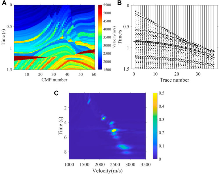
FIGURE 6. (A) True interval velocity field, (B) 40th CMP seismic records of synthetic data without noise, and (C) 40th velocity spectrum of synthetic data without noise.

FIGURE 7

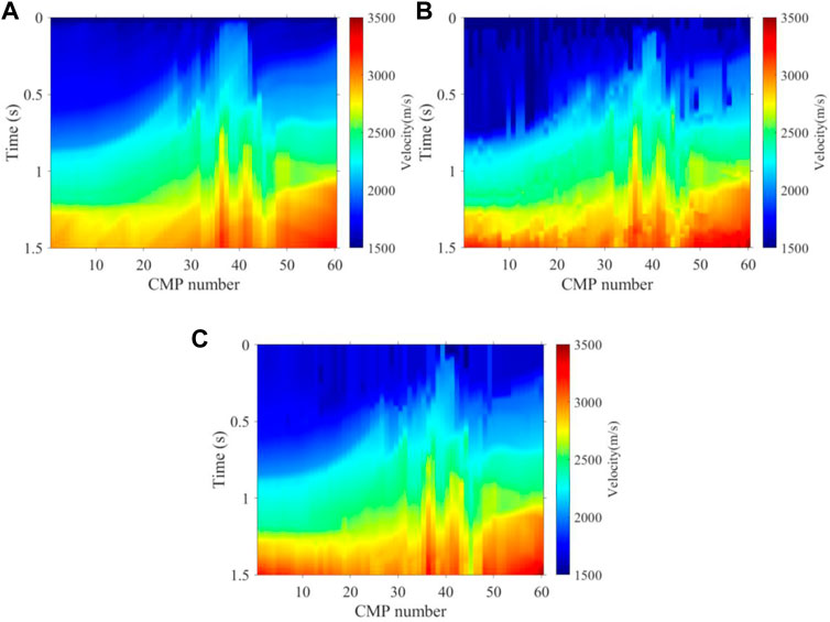
FIGURE 7. Stacking velocity field of synthetic data without noise. (A) True velocity, (B) K-means intelligent picking velocity, and (C) intelligent picking velocity by the method proposed.

Figure 7B and Figure 7C show the two-dimensional stacking velocity of traditional K-means and the method we proposed, respectively, which are combined with the 60 picked curves of the 60 velocity spectra. Every 10 velocity spectra are constrained by an expert experience. In general, the two-dimensional stacking velocity field obtained by our method is basically consistent with the real velocity field shown in Figure 7A on the tectonic trend, while the one with K-means contains a lot of background noise and incorrect construction. Compared to the two-dimensional stacking velocity field of K-means, our method is more continuous and stable, since almost all the velocity spectra energy clusters are picked correctly just like the real velocity spectra. In detail, local structures such as a deep high-velocity body and shallow weak reflection interface in the velocity field are also well portrayed by using our method. In seismic data processing, the higher the accuracy of the velocity field, the more realistic the stacked tectonic profile obtained is, and then the subsurface structure is reflected more accurately. In addition, we made an NMO stack using seismic records and the three velocity fields in Figure 7 for further comparison in the tectonic profile, and the stacked tectonic profiles are shown in Figure 8. Compared to the K-means profile, the profile obtained by our method is closer to the real structure shown in Figure 8A, and hence both the shallow and deep structures’ imaging accuracy of our method is higher than the K-means. With regards to efficiency, compared to the time required for manual picking, our method is very efficient. It takes only approximately 1 s to pick up one velocity spectrum, which significantly improves the efficiency similar to the K-means method, but our method has a highly accurate structure imaging result.

FIGURE 8

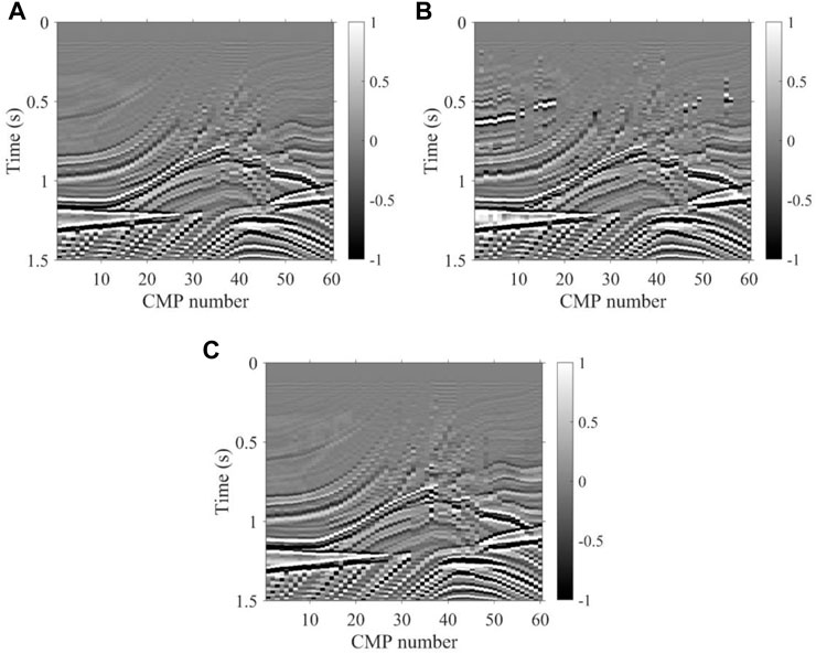
FIGURE 8. Stacking profiles of synthetic data without noise. (A) True velocity, (B) velocity of K-means, and (C) velocity of the method proposed.

In order to test the noise immunity of our proposed method, we tested the 2D Marmousi model, from which the seismic records have 30% random noise, and the velocity spectra from the seismic records had 30% random noise and, additionally, strong energy regular noise rotated by valid energy clusters, as shown in Figure 9A, B. Compared to the velocity field of K-means, as shown in Figure 10B, the velocity field obtained by our method shown in Figure 10C is more consistent with the real velocity shown in Figure 10A on the overall trend; therefore, we can see that the K-means velocity has a large error both in the shallow and deep regions of the velocity field. In addition, we made an NMO stack using seismic records and the three velocity fields of Figure 10 for further comparison from the tectonic profile. As shown in Figure 11, the stack profile obtained by our method still has a higher accuracy in structure imaging than the K-means, especially for the deep region. The test results show that our method could obtain better noise immunity. This means that our method is better adapted to real noise-bearing seismic data in the field.

FIGURE 9

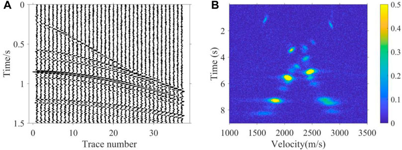
FIGURE 9. (A) 40th CMP seismic records of synthetic data with random noise. (B) 40th velocity spectrum of synthetic data with random noise and strong energy regular noise.

FIGURE 10

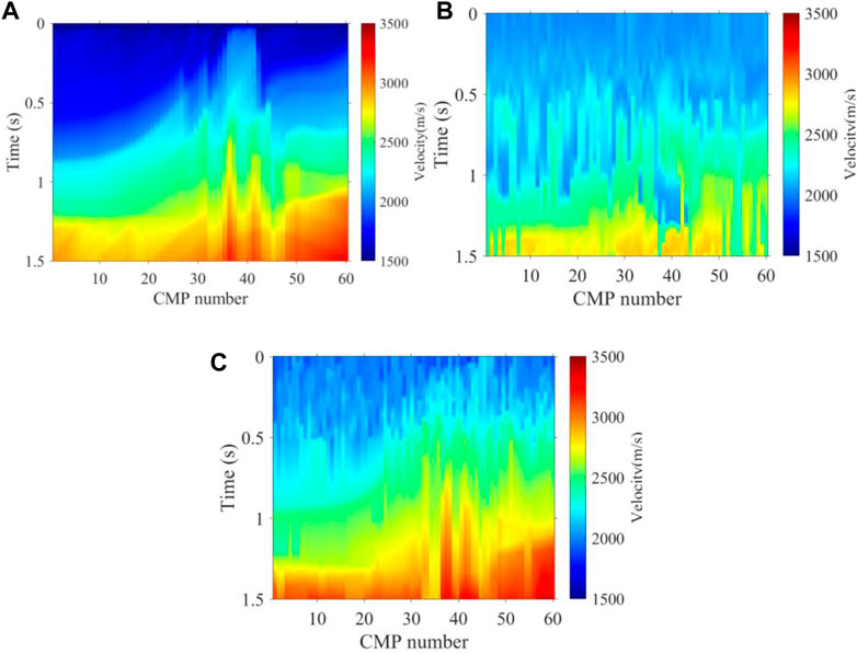
FIGURE 10. Stacking velocity field of synthetic data with random noise and strong energy regular noise. (A) True velocity, (B) K-means intelligent picking velocity, and (C) intelligent picking velocity by the method proposed.

FIGURE 11

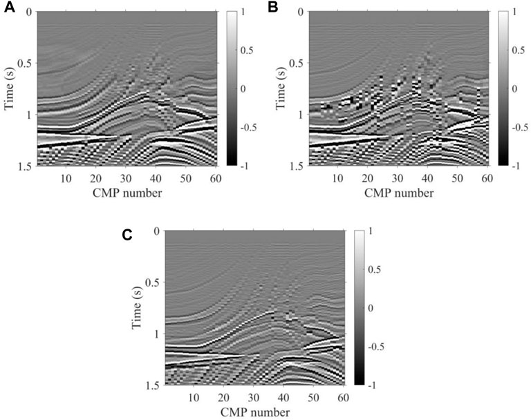
FIGURE 11. Stacking profiles of synthetic data with random noise and strong energy regular noise. (A) True velocity, (B) velocity of K-means, and (C) velocity of the method proposed.

3.2 Real data

To further verify the applicability of the method we proposed, 2D land data with 4,880 velocity spectra (CMPs) were first picked up manually and then picked up intelligently by using K-means and our method. There are often many energy clusters in the CMP velocity spectrum of seismic data. In fact, these energy clusters are generated by effective primary reflection seismic waves and interference multiple reflection waves, each energy cluster corresponding to one velocity value at that time. Compared to the energy clusters of primary reflection waves, the interference energy clusters generated by these multiple waves are often located at a lower velocity (near the left side of the velocity spectrum). In the process of manual velocity picking by the processors, it is necessary to identify and discard the energy clusters generated by multiple reflection waves to avoid false structures in the subsequent velocity field and stack profile. Compared to traditional unsupervised clustering methods, such as K-means, our method introduces expert experience to evade the energy clusters in the deep region of the velocity spectrum generated by the multiples in the real data so as to achieve the accuracy of manual picking, while the K-means incorrectly picks up the energy clusters of multiples and makes some false structures on the subsequent velocity field and stack tectonic profile. The 3900th velocity spectrum with multiples developing at 6–9 s shown in Figure 4A is one of the 4,880 velocity spectra. In fact, after the 3500th velocity spectrum, this real data has obvious multiple interference signals. Expert experience constraints are performed every 500 velocity spectrums when we performed the intelligent velocity picking method we proposed.

As shown in Figure 12 and Figure 13, the 3500th and 4300th velocity spectrum of the land data are processed by experts, the K-means method, and the method we proposed. Obviously, our method can effectively avoid the interference of multiples, which conforms to the trend of manual picking, while the K-means regard the multiples as effective signals to be picked up. Figure 14 shows the picking results of the 100th velocity spectrum (CMP). The signal-to-noise ratio of the velocity spectrum is low, and it is difficult to see effective energy clusters. However, our method can maintain consistency with the trend of manual results, as shown in Figure 14A, due to the expert experience constraints, while the K-means results are abnormal. Figure 15 shows the velocity field of this 2D real data constructed by manual picking, K-means, and our method. It is found that the velocity field established by K-means is significantly different from the manual velocity field, and its accuracy is seriously affected by the interference multiples. However, the velocity field established by our method has the same trend and structure as the manual one both in the shallow and deep regions, and at the same time, the efficiency of our method is much faster than that of manual picking, as it only takes about 1 s to pick up one velocity spectrum while manual picking takes at least 30 s. As a whole, compared to unsupervised clustering methods, such as K-means, our method can better replace experts to pick up the velocity spectrum, which improves efficiency and frees manpower, while meeting the picking accuracy.

FIGURE 12

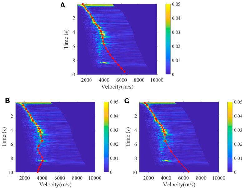
FIGURE 12. Velocity function of the 3500th velocity spectrum obtained by (A) manual, (B) K-means, and (C) the method proposed.

FIGURE 13

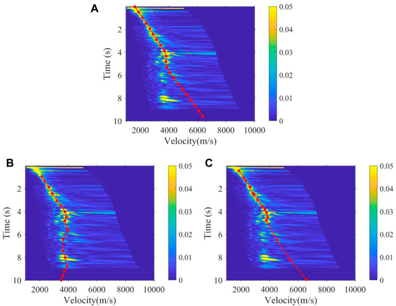
FIGURE 13. Velocity function of the 4300th velocity spectrum obtained by (A) manual, (B) K-means, and (C) the method proposed.

FIGURE 14

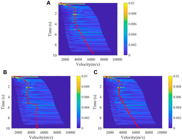
FIGURE 14. Velocity function of the 100th velocity spectrum obtained by (A) manual, (B) K-means, and (C) the method proposed.

FIGURE 15

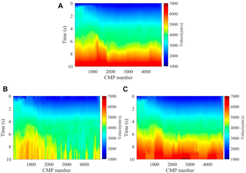
FIGURE 15. Velocity field of a 2D real data established by (A) manual, (B) K-means, and (C) the method proposed.

In addition, for a more intuitive comparison, we made an NMO stack with the three velocity fields in Figure 15 for further comparison in the tectonic profile, and as shown in Figure 16C, the subsurface structure imaging profile of K-means has fuzzy structures in the shallow red frame and false structures caused by multiples in the deep red frame. However, the profiles of our method and manual are the same as each other, both in the shallow and mid-deep layers, and the subsurface imaging results of them can provide references for subsequent geological understanding. Moreover, since our method can pick up velocity spectra one by one owing to the significantly decreased picking time, the profile of our method even has a better imaging performance in the local positions than the manual one at the red arrows in Figure 17A, B, where the weak reflection events are strengthened and are more continuous. For the K-means, its stack tectonic profile loses some important structures, especially in the deep region, as shown in the red frame of Figure 17C. All in all, from the tectonic profile, our method has better image results than those of the manual and K-means; hence, the method we proposed improves efficiency, frees up manpower, and can better replace experts to pick up the velocity spectrum automatically.

FIGURE 16

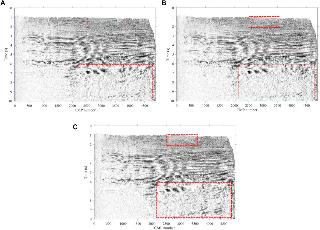
FIGURE 16. Stacking profiles of (A) manual, (B) method proposed, and (C) K-means.

FIGURE 17

FIGURE 17. Local enlarged stacking profiles of (A) manual, (B) method proposed, and (C) K-means.

4 Conclusion

Up to now, manual velocity picking in seismic data processing was the primary way; however, it is labor-intensive and repetitive. An intelligent velocity picking method considering the expert experience based on the Chan–Vese model and mean-shift clustering is proposed by imitating the process of manual velocity picking so as to improve efficiency and free up manpower. In our method, the valid velocity energy clusters are identified by using the CV model with expert experience constraints, which corresponds to the first step of manual picking. Meanwhile, the clustering of the valid energy clusters corresponds to the second step of manual picking by using the mean-shift clustering method. These two steps translate geophysical and geological theories into the geometry of energy clusters on the velocity spectrum. The theoretical model and actual data test prove that our method has several advantages as can be seen in the following paragraph.

Compared to the manual and K-means, the method we proposed can obtain a highly accurate velocity field and subsurface tectonic imaging profile, which can provide a better reference for subsequent geological understanding, while the K-means method always falls into the wrong picking result. In terms of efficiency, our method takes only approximately 1s to pick up one velocity spectrum similar to other automatic methods such as K-means, while manual picking takes at least 30 s. All in all, our method can replace manual velocity picking by experts, which improves efficiency, frees up manpower, and enhances picking accuracy.

Data availability statement

The raw data supporting the conclusion of this article will be made available by the authors, without undue reservation.

Author contributions

L-DW is the main author of the research results; JW and X-RX provided auxiliary support; and H-HZ, YG, and W-QL applied and tested the results.

Funding

This study was supported by the science and technology project of PetroChina: Research and Field Tackling Test of Artificial Intelligence Seismic Reservoir Carving Technology (2022KT1501) and Subsalt Seismic Imaging Tackling and Target Implementation in the Cambrian Subsalt System at the Periphery of the Hotan River and Tarim Basin (2022KT0506).

Conflict of interest

The authors L-DW, JW, X-RX, H-HZ and W-QL were employed by the Research Institute of Petroleum Exploration & Development-Northwest (NWGI), PetroChina.

The remaining author declares that the research was conducted in the absence of any commercial or financial relationships that could be construed as a potential conflict of interest.

Publisher’s note

All claims expressed in this article are solely those of the authors and do not necessarily represent those of their affiliated organizations, or those of the publisher, the editors, and the reviewers. Any product that may be evaluated in this article, or claim that may be made by its manufacturer, is not guaranteed or endorsed by the publisher.

References

Aghamohammadi, A., Ranjbarzadeh, R., Naiemi, F., Mogharrebi, M., Dorosti, S., and Bendechache, M. (2021). Tpcnn: Two-path convolutional neural network for tumor and liver segmentation in CT images using a novel encoding approach. Expert Syst. Appl 183, 115406. doi:10.1016/j.eswa.2021.115406

CrossRef Full Text | Google Scholar

Agudelo, W., Villa, Y., Duarte, C., and Sierra, D. (2017). Seismic attribute selection and clustering to detect and classify surface waves in multicomponent seismic data by using k-means algorithm. Lead. edge 36 (3), 239–248. doi:10.1190/tle36030239.1

CrossRef Full Text | Google Scholar

Araya-Polo, M., Dahlke, T., Frogner, C., Zhang, C., Poggio, T., and Hohl, D. (2017). Automated fault detection without seismic processing. Lead. edge 36 (3), 208–214. doi:10.1190/tle36030208.1

CrossRef Full Text | Google Scholar

Biswas, R., Vassiliou, A., Stomberg, R., and Sen, M. K. (2019). Estimating normal moveout velocity using the recurrent neural network. Interpretation 7 (4), T819–T827. doi:10.1190/int-2018-0243.1

CrossRef Full Text | Google Scholar

Cameron, M., Fomel, S., and Sethian, J. (2008). Time-to-depth conversion and seismic velocity estimation using time-migration velocity. Geophysics 73 (5), 205–210. doi:10.1190/1.2967501

CrossRef Full Text | Google Scholar

Cao, W., Guo, X. B., Tian, F., Ying, S., Wei-Hong, W., and Hong-Ri, S., (2022). Seismic velocity inversion based on CNN-LSTM fusion deep neural network. Appl. Geophys 18 (4), 499–514. doi:10.1007/S11770-021-0913-3

CrossRef Full Text | Google Scholar

Chen, Y. Q., (2018). Automatic semblance picking by a bottom-up clustering method. SEG Maximizing Asset Value Through Artif. Intell. Mach. Learn, 44–48. doi:10.1190/AIML2018-12.1

CrossRef Full Text | Google Scholar

Comaniciu, D., and Meer, P. (2002). Mean shift: A robust approach toward feature space analysis. IEEE Trans Pattern Analysis Mach. Intell 24 (5), 603–619. doi:10.1109/34.1000236

CrossRef Full Text | Google Scholar

Fabien-Ouellet, G., and Sarkar, R. (2020). Seismic velocity estimation: A deep recurrent neural-network approach. Geophysics 85 (1), U21–U29. doi:10.1190/geo2018-0786.1

CrossRef Full Text | Google Scholar

Getreuer, P. (2012). Chan-vese segmentation. Image Process. Line 2, 214–224. doi:10.5201/ipol.2012.g-cv

CrossRef Full Text | Google Scholar

Goodfellow, I., Bengio, Y., and Courville, A. (2016). Deep learning. The MIT Press. Cambridge, MA, USA, doi:10.1007/s10710-017-9314-z

CrossRef Full Text | Google Scholar

Hou, A., and Marfurt, K. J. (2002). Multicomponent prestack depth migration by scalar wavefield extrapolation. Geophysics 67 (6), 1886–1894. doi:10.1190/1.1527088

CrossRef Full Text | Google Scholar

Jones, I. F., Ibbotson, K., Grimshaw, M., and Plasterie, P. (1998). 3-D prestack depth migration and velocity model building. Lead. Edge 17 (7), 897–906. doi:10.1190/1.1438063

CrossRef Full Text | Google Scholar

Keegan, M. S., Sandberg, B., and Chan, T. (2017). A multiphase logic framework for multichannel image segmentation. Inverse Problems Imaging 6 (1), 95–110. doi:10.1109/34.537343

CrossRef Full Text | Google Scholar

LeCun, Y., Bengio, Y., and Hinton, G. (2015). Deep learning. Nature 521 (7553), 436–444. doi:10.1038/nature14539

PubMed Abstract | CrossRef Full Text | Google Scholar

Li, Q., Pan, Z. K., Wei, W. B., and Song, T. T. (2021). Fast segmentation methods for convex relaxation chan-vese model. Comput. Simul 38 (06), 226–232. doi:10.3969/j.issn.1006-9348.2021.06.047

CrossRef Full Text | Google Scholar

Martin, G. S., Wiley, R., and Marfurt, K. J. (2006). Marmousi2: An elastic upgrade for Marmousi. Lead. Edge 25 (2), 156–166. doi:10.1190/1.2172306

CrossRef Full Text | Google Scholar

Nemeth, T., Wu, C. J., and Schuster, G. T. (1999). Least-squares migration of incomplete reflection data. Geophysics 64 (1), 208–221. doi:10.1190/1.1444517

CrossRef Full Text | Google Scholar

Osher, S., and Sethian, J. A. (1988). Fronts propagating with curvature-dependent speed: Algorithms based on Hamilton-Jacobi formulations. J. Comput. Phys 79 (1), 12–49. doi:10.1016/0021-9991(88)90002-2

CrossRef Full Text | Google Scholar

Park, M. J., and Sacchi, M. D. (2020). Automatic velocity analysis using convolutional neural network and transfer learning. Geophysics 85 (1), V33–V43. doi:10.1190/geo2018-0870.1

CrossRef Full Text | Google Scholar

Ranjbarzadeh, R., Bagherian, K. A., Jafarzadeh, G. S., Anari, S., Naseri, M., and Bendechache, M. (2021). Brain tumor segmentation based on deep learning and an attention mechanism using MRI multi-modalities brain images. Sci. Rep 11, 10930. doi:10.1038/s41598-021-90428-8

PubMed Abstract | CrossRef Full Text | Google Scholar

Ranjbarzadeh, R., Tataei, S. N., Jafarzadeh, G. S., Saleh Esfahani, M., Parhizkar, M., and Pourasad, Y., (2022). MRFE-CNN: Multi-route feature extraction model for breast tumor segmentation in Mammograms using a convolutional neural network. Ann. Oper. Res. doi:10.1007/s10479-022-04755-8

CrossRef Full Text | Google Scholar

Rumelhart, D. E., Hinton, G. E., and Williams, R. J. (1986). Learning representations by back-propagating errors. Nature 323 (6088), 533–536. doi:10.1038/323533a0

CrossRef Full Text | Google Scholar

Toldi, J. L. (1989). Velocity analysis without picking. Geophysics 54 (2), 191–199. doi:10.1190/1.1442643

CrossRef Full Text | Google Scholar

Velis, D. (2021). Simulated annealing velocity analysis: Automating the picking process. Geophysics 86 (2), V119–V130. doi:10.1190/geo2020-0323.1

CrossRef Full Text | Google Scholar

Waheed, U. B., Al-Zahrani, S., and Hanafy, S. M. (September, 2019). Machine learning algorithms for automatic velocity picking: K-Means vs. DBSCAN. Proceedings of the SEG Technical Program Expanded Abstracts. San Antonio, Tx, USA,

Google Scholar

Wang, D., Yuan, S. Y., Liu, T., Li, S. J., and Wang, S. X. (2021a). Inversion-based non-stationary normal moveout correction along with prestack high-resolution processing. J. Appl. Geophys 191, 104379. doi:10.1016/j.jappgeo.2021.104379

CrossRef Full Text | Google Scholar

Wang, D., Yuan, S. Y., Yuan, H., Zeng, H. H., and Wang, S. X. (2021b). Intelligent velocity picking based on unsupervised clustering with the adaptive threshold constraint. Chin. J. Geophys 64 (3), 1048–1060. doi:10.6038/cjg2021O0305

CrossRef Full Text | Google Scholar

Wang, W. L., McMechan, G. A., Ma, J. W., and Xie, F. (2020). Automatic velocity picking from semblances with a new deep-learning regression strategy: Comparison with a classification approach. Geophysics 86 (2), U1–U13. doi:10.1190/geo2020-0423.1

CrossRef Full Text | Google Scholar

Wang, X., Liu, H., and Ma, W. L. (2018). Sparse least squares support vector machines based on Meanshift clustering method. IFAC-PapersOnLine 51 (18), 292–296. doi:10.1016/j.ifacol.2018.09.315

CrossRef Full Text | Google Scholar

Wang, X. W., Gao, Y., Chen, C., Yuan, H., and Yuan, S. (2022). Intelligent velocity picking and uncertainty analysis based on the Gaussian Mixture Model. Acta Geophys 70, 2659–2673. doi:10.1007/s11600-022-00859-8

CrossRef Full Text | Google Scholar

Wilson, H., and Gross, L. (2019). Reflection-constrained 2D and 3D non-hyperbolic moveout analysis using particle swarm optimization. Geophys. Prospect. 67, 550–571. doi:10.1111/1365-2478.12758

CrossRef Full Text | Google Scholar

Yuan, S. Y., Jiao, X. Q., Luo, Y. N., Sang, W. J., and Wang, S. X. (2022). Double-scale supervised inversion with a data-driven forward model for low-frequency impedance recovery. Geophysics 87 (2), R165–R181. doi:10.1190/geo2020-0421.1

CrossRef Full Text | Google Scholar

Yuan, S. Y., Wang, S. X., Luo, Y. N., Wei, W. W., and Wang, G. C. (2019). Impedance inversion by using the low-frequency full-waveform inversion result as an a priori model. Geophysics 84 (2), R149–R164. doi:10.1190/geo2017-0643.1

CrossRef Full Text | Google Scholar

Zhang, H., Zhu, P. M., Gu, Y., and Li, X. Z. (September, 2019). Automatic velocity picking based on deep learning. Proceedings of the SEG Technical Program Expanded Abstracts, San Antonio, Tx, USA, 2604–2608. doi:10.1190/segam2019-3215633.1

CrossRef Full Text | Google Scholar

Zhang, P., Lu, W., and Zhang, Y. (2015). Velocity analysis with local event slopes related probability density function. J. Appl. Geophys 123, 177–187. doi:10.1016/j.jappgeo.2015.10.010

CrossRef Full Text | Google Scholar