Modeling and estimation of snow depth spatial correlation structure from observations over North America

Estimation of spatial correlations should be an integral part of objective analysis of geophysical variables. However, a statistical assessment of spatial correlations has been absent from studies of objective analysis of snow depth since its debut over 2 decades ago. We show a method for computing regional spatial correlations of observed snow depth and the daily snow depth increment and fitting them to correlation functions to estimate the correlation scale parameters. Both horizontal and vertical distance correlations are computed from station observations over a well sampled part of North America. The vertical and horizontal distance correlations are fitted to exponential functions using the least square method to estimate the correlation scale parameters including the amplitude, which represents short distance correlation. Our assessment suggests a large horizontal e-folding correlation scale for both the observed snow depth and the daily increment, with implications for improving predictions in poorly monitored areas with relatively flat topography. Over mountainous terrain, vertical e-folding correlation scale for observed snow depth is much smaller than that for the daily snow depth increment and for the snow depth increment used in operational snow analyses. That means that optimal interpolation-based analysis of the increments may be more accurate than the interpolation of snow depth data.

1 Introduction

Spatial distribution of snow depth exhibits long spatial correlations, which can be exploited for regional mapping of snow depth using Kriging interpolation method. Kriging requires the specification of the spatial correlation functions which the technique uses to compute the spatial correlations between pairs of observations and between each observation and the grid point being considered for estimation. These spatial correlation values are then used to compute the weight of each observation and the grid point snow depth as a spatially weighted average. Spatial correlation functions of the analysis snow depth increment, defined as the difference between the observed snow depth and a first guess snow depth estimate, have been used in Optimal Interpolation (OI), a variant of Kriging, for global (re)analysis of snow depth at world’s major weather and climate prediction centers (Brasnett, 1999; Brown et al., 2003; de Rosnay et al., 2012; JMA, 2019) and for blending of satellite with in situ snow depth observations (Liu et al., 2015; Kongoli et al., 2019; Gan et al., 2021). In those studies, the interpolated variable is the analysis snow depth increment, for which a short-term weather forecast or a satellite estimate represents the first guess, and in this case the correlation functions describe the spatial correlation structure of the analysis snow depth increments.

A central assumption of Kriging/OI method is that the embedded correlation functions represent the spatial correlation structure of the interpolated variable for the method to be optimal and for the spatial weights to have realism, in our case, to estimate snow depth with minimum error and with an accuracy significantly higher than the simple average. Therefore, fitting observations to the correlation functions to estimate the function parameters should be an integral part of Kriging/OI-based analysis.

In operational OI-based snow depth analyses, the spatial correlations of the analysis snow depth increments are computed using the family of exponential correlation functions as follows:

$C=AC\left(d\right)C\left(z\right)(1)$

$C\left(d\right)=\left(1+\alpha d\right)\mathit{exp}\left(-\alpha d\right)(2)$

$\mathrm{C}\left(\mathrm{z}\right)=\exp \left(-{\left(\frac{z}{h}\right)}^2\right)(3)$

where d and z are horizontal and vertical distance between observations in km and m, respectively, C in Eq. 1 is the analysis snow depth increment correlation, expressed as a product between the horizontal C(d) and vertical C(z) distance correlation functions (Eqs 2, 3). The parameters A, α, h are fixed at 1.0, 0.018 km⁻¹, 800 m, respectively. From these values, the horizontal e-folding scale parameter α⁻¹ is 55.60 km (computed as 1/0.018), which yields an effective e-folding snow depth distance, i.e., the horizontal distance at which the analysis increment correlation drops to e⁻¹, about 120 km. The vertical e-folding scale parameter h yields the same effective e-folding snow depth distance of 800 m. A is the amplitude, defined as the correlation as the separation distance approaches zero. The amplitude reflects noise from measurement and sampling errors, and with little noise its value is close to one while noise lowers the amplitude.

The correlation functions and the scale parameters as above indicated were suggested by Brasnett (1999). A limitation arises in cases where the separation distance between observations is much larger than the horizontal e-folding scale of 120 km. When these distant observations are used for interpolation, the increment correlations estimated from Eq. 2 would be close to zero, which means that the increments can be considered uncorrelated, and the interpolated value would be estimated close to the simple average. Kongoli et al. (2019) considered a maximum range of 600 km for the snow depth analysis to have sufficient coverage of observations over all of North America. The maximum range needs to be increased even more than 600 km in other remote areas of the globe without a significant benefit of using Kriging/OI. In areas with significant gaps in observations the analysis relies heavily on the first guess snow depth. Large analysis errors were found over the mountains of Western North America compared to those over relatively flat eastern regions, which could in part be the result of inaccurate modeled vertical correlation scales. Liu et al., 2015 used Eqs 1–3 and Brasnett (1999) parameter values to compute the increment correlations for blending satellite-estimated snow depth with in situ snow depth over Upper Colorado Basin in Western US. They only considered stations for interpolation with an elevation difference from the interpolated grid point less than 300 m, in order to minimize errors that might arise from a much smaller vertical correlation scale of snow depth than the 800 m model e-folding scale.

When analysis increment correlation scales were chosen over 2 decades ago there was much less information available for their estimation. The accumulation of snow depth data since then gives an opportunity to consider launching statistical assessments of the spatial snow depth correlations. This study presents a method for computing regional spatial correlation statistics of observed snow depth and the daily snow depth increments over a well sampled part of North America. Specifically, correlations are computed from in situ snow depth and fitted to correlation functions of horizontal and vertical distance to estimate the horizontal and vertical scale parameters including the amplitude. We evaluate how well the exponential functions used in snow depth analysis represent the correlations of observations over North America.

In this regard, it is important to make the distinction between the observed snow depth and the analysis snow depth increment correlation statistics. In the latter case, the statistics depend on both the specific model used to produce the first guess snow depth and the sampling of snow depth observations. This study focuses on the correlations of observed snow depth and the daily snow depth increments, the latter defined as the difference between observed snow depth on a given day and that from the previous day. We chose to focus on the correlation statistics of observations because knowledge of spatial correlations of observations would be useful for a wider range of hydro-meteorological applications and employment of improved correlation functions and scale parameters based on observations has the potential for improving operational snow analyses.

2 Data and methodology

2.1 Estimation of correlations from observations

2.1.1 Data collection and the study region

Correlations are computed separately for snow depth and the daily snow depth increment using snow depth observations from December, January, and February (DJF) for the years 2012–2016. For each day the daily snow depth increment is defined as the difference between the daily value and the value of the previous day. A snow depth must be defined at each location for both days for a daily change to be defined for use in computing statistics.

Daily snow depth is obtained from NOAA’s Global Historical Climatology Network (GHCN)-Daily, available at NOAA’s National Center for Environmental Information (NCEI, https://www.ncdc.noaa.gov). The database represents the most comprehensive collection of US station data, and it includes numerous other sources such as Environmental Canada and European Climate Assessment and Dataset. Quality assurance of daily observations consists of a series of automated tests and semi-automatic checks by trained validators. Automated tests for daily snow depth change include statistical tests for the detection of excessively large values, for unrealistic occurrences when recorded air temperatures are warmer than a threshold and for daily snowfall which exceed recorded solid precipitation. Station snowfall/snow depth is tested for false positive snow, e.g., over warmer regions or seasons for which snow is impossible, and for anomalously large breaks in the distribution of snow depth monthly records. For an overview of GHCN-Daily and further details on quality checks, the reader is referred to Durre et al., 2008; Durre et al., 2010, Menne et al., 2012 and to the NCEI website.

For DJF months, correlations are computed over North America where stations are densest (30°N-55°N). Figure 1 depicts the snow sampling density of GHCN-Daily stations over the study region. As shown, the fraction of days sampled over DJF in these years tends to be higher in snowier regions, as expected, since there is only a report if there is snow (zero snow depth is not reported). In the snowier regions such as over high elevation areas of Western US the fraction can be relatively high, 0.7 to 0.9, although the spatial density of stations is lower than over south-central and south-eastern US. Over less snowy regions the fraction is typically 0.1 to 0.2 although station density is higher. Snow reaching the far southern areas is not uncommon, but when it happens it does not persist for extended periods due to rapid melting from a warm climate.

FIGURE 1

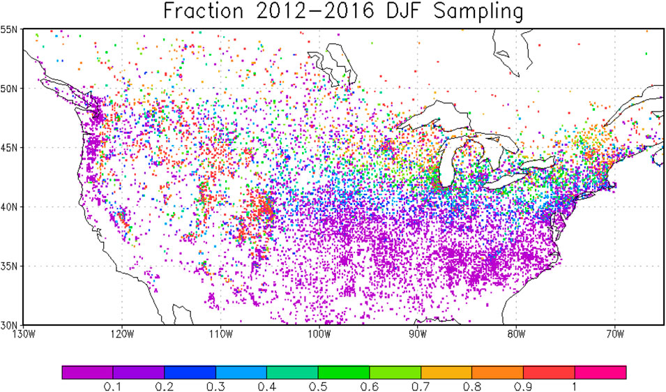
FIGURE 1. The study region (30°N-55°N). Depicted is the fraction of days in DJF months for the GHCN stations over 2012–2016 with snow-depth sampling. Sampling = 1 if all days are sampled.

GHCN-Daily weather station density over the study domain is one of the highest globally, with greater than 100 snow depth measuring stations per 5° grid (Jaffrés, 2019). For the high mountain areas located west of 100° longitude, stations reporting daily snow depth were distributed evenly througlout the study period across the low (500–1,000 m), medium (1,000–2,000 m) and high (greater than 2,000 m) elevation bands. The daily station count was the lowest for stations with elevation less than 500 m, about 5% of the daily total, reflecting the much smaller extent of snow cover relative to higher elevation sites. On average, the number of stations reporting a (positive) daily snow depth value was 1,700 per day. Daily, seasonal and annual variations in station count reflected mostly the changes in snow cover distribution. East of the 100° longitude, the mean number of stations reporting a snow depth value was about 2,100 per day. The fluctuations in daily count were larger compared to the west, driven by more rapid changes in snow cover distribution.

2.1.2 Technique for computing observed correlations

Both horizontal and vertical (altitude-dependent) correlations are considered. The goal of this step is to compute correlations from observations for a range of horizontal and vertical distances that can then be fitted to correlation functions of horizontal distance and to correlation functions of vertical distance. To this end, we divide the geographical extent of the study depicted in Figure 1 into two sub-regions, one for computing the horizontal correlations and the other for computing the vertical correlations, to control for the influence of one predictor on the other. Additionally, we perform binning of distances in computing correlations, to average out the heterogeneity in spatial dependence of correlation on separation distance between irregularly spaced stations.

Horizontal correlation statistics are computed using daily data from 30°N-55°N, 100°W-65°W, east of the greatest elevation changes over North America, with the assumption that elevational changes over this region have negligible influence on horizontal correlations. Vertical correlation statistics are computed using daily data from 30°N-55°N and west of 100°W, where elevation changes are greatest. As described below, to compute vertical correlation statistics, we developed a method that minimizes the influence of horizontal separation on vertical correlations.

For computing binned horizontal correlations from unevenly distributed stations, we resample observations into a grid in which the horizontal distance between observations is measured by the distance between centers of their grid boxes. Inspection of the daily data revealed that 0.1° by 0.1° spatial grid represents a fine spatial resolution of the daily data over this sub-region, in that most grid boxes of this size there is only one observation. In the few grid squares with more than one observation, we use only the first one for consistency. Squares with no stations are not filled. Using station data on this fine grid allows the binned correlations to be more easily computed. Since correlation scales are much larger than the grid scale, any uncertainty associated with this method should be minimal. A coarse grid box with a size comparable to that of the e-folding scale would fail to detect the intrinsic correlation structure of snow depth. That could be the case, for example, if this technique is applied over a region with sparse observations.

Horizontal correlations are computed with distance for bins 10 km wide, which is approximately the size of each grid square, with distances of 0 < d ≤ 10 km, …, 490 km < d ≤ 500 km. The lag distances for which correlations (referred to hereafter as “lag correlations”) are computed are 5, 15, …. 495 km, the distances between the mid points of the 10 km wide bins. The horizontal scales computed are isotropic, since it would be difficult to get greater detail from computations over this relatively small region. The computational procedure is as follows: For a square grid box with an observation present (referred to as “the base”), lag correlations are computed by looping through the grid squares with observations present, to find all same-day pairs of observations with the same lag distance from the base. Next, these pairs of observations are pooled to compute one lag correlation value for each lag distance from the base. This process is repeated to compute lag correlations for all the grid boxes with observations present. Note that only lag correlations are computed, and only when lag data, i.e., grid squares with observations, are available. These lag correlations are later fit to lag-correlation equations to estimate scale parameters, including the e-folding scale and the correlation as the lag approaches zero. The fitting to equations is discussed in the next section.

The method for computing lag correlations described above is similar to the usual way the empirical semi-variogram is modelled, whereby smoothing of the measured semi-variances is achieved by the binning of irregular distances between observations into distance classes of equal width and pooling of the data with the same lag distance to compute semi-variances. This averaging process which we chose to apply is described in Webster and Oliver (2007), Chapter 4). Another way of computing lag correlations (which we did not use) is the following: correlations are computed first, between a station, in our case, a base grid box, and each of the stations/grid boxes with observations present. Next, these individual correlations with the same lag distance are averaged. This method is suggested in Thiébaux and Pedder (1987), Chapter 4). When scales are assumed isotropic as in our study, pooling of the surrounding observations from a base with the same lag distance provides larger correlation samples than those for computing individual correlations, especially over less snowy regions. In these regions, such as in the southern US, stations have shorter records and samples with station observations are smaller, and we do not exclude these stations from computations unless the sample size for computing binned correlations is less than 20, which we use as the minimum threshold for samples to be considered for analysis.

For the vertical lag correlations, data are compared for adjacent grid squares: there are too few stations in one grid box at different elevations to compute vertical correlations over same grid box, so it is necessary to use stations separated by one grid square. As with the horizontal lag correlations, the vertical lag correlations are computed using only one station observation per grid square. Several experiments are performed to find out how much horizontal separation is needed in the stations to compute vertical correlations. Here we use data within 0.1° of a central grid in computations. This horizontal separation has negligible effect on vertical correlations since it is much smaller than the horizontal scales. Therefore, consideration of adjacent grid squares of this size is a reasonable strategy in computing vertical correlations. Vertical distances that correlations are computed for are bins of 100 m width. Distances considered are 0 < d ≤ 100 m, …, 4,900 m < d ≤ 5,000 m, and lag distances are 50, 150, …, 4,950 m. As with the horizontal correlations, all distances within a given bin are treated as the same for computing the fits.

Lagged vertical correlations from a base grid box with observations are computed by searching only over the adjacent grid squares for all pairs of observations with same vertical lag distance from that base. Next, the data are pooled to compute one vertical lag correlation value from the base. In a similar fashion, the search continues over all grid squares with observations.

2.2 Estimation of scale parameters

The binned correlation values computed for observed snow depth and the daily snow depth increment are fit to Eqs 2, 3 modified to estimate the amplitude A and the correlation scale α from the fits. Note that Eq. 3 can also be expressed using the correlation scale α instead of the e-folding scale h, since α is equal to h⁻¹. Scales are assumed to be fixed parameters for the total area under consideration.

Three scenarios are evaluated by comparing how well the selected equation represents the observed correlation with (vertical or horizontal) distance: the autoregressive correlation function (Eq. 2) with an amplitude equal to 1.0, the autoregressive correlation function (Eq. 2) with an amplitude estimated from the fit to observed correlations, and the exponential correlation function (Eq. 3) with an amplitude estimated from the fit to observed correlations. In each scenario, α is estimated from the fit. The three equations are fit to four separate observed correlations: Observed horizonal and vertical correlations for the snow depth and for the daily snow depth increment. Note that each of the correlation equations are fit to the same observational set, to intercompare the equation fits for each of the four relationships. The results are discussed in the next section. In this section we describe the correlation functions and the mathematical transformations necessary for carrying out numerical computations to estimate the scale parameters.

The observed correlations with distance are denoted $C_o\left(d\right)$. For each of the three equations tested the equation-fit correlation with distance is $C_k\left(d\right)$, for k = 1, 2, 3. Each is a fit to the same observations. Equations for each of the k fits are solved to minimize the mean-squared error (MSE) of the fit averaged over all the binned distances. That is done by differentiating the mean-squared difference with respect to the fitting parameters and setting that to zero, for example

$\frac{\partial }{\partial {\alpha }_k}〈{\left(C_k-C_o\right)}^2〉=0.(4)$

Here the angle brackets denote averaging. If the function fit uses only an e-folding scale, $S_k$, the parameter is ${\alpha }_k=S_k^{-1}$. For two of the fits there is also an amplitude parameter, $A_k$. In those cases, both parameters are estimated to minimize the MSE of the fit.

The first fit considered, referred to as Fit1, is the one used by Brasnett (1999), to model horizontal analysis snow depth increment correlations using an amplitude equal to 1.0,

$C_1=\left(1+d{\alpha }_1\right)\mathit{exp}\left(-d{\alpha }_1\right).(5)$

The function is a second-order autoregressive function also suggested for analysis of a background field (Thiébaux 1985; Daley 1991). Substituting C_k in Eq. 4 with the right-hand expression of Eq. 5, taking the first derivate of the MSE of Eq. 4 with respect to ${\alpha }_1$ and setting it to zero yields

$〈\left(1+{\alpha }_{1}d\right)d^2\mathit{exp}\left(-2{\alpha }_{1}d\right)〉-〈C_o{d}^2\mathit{exp}\left(-{\alpha }_{1}d\right)〉=0.(6)$

A solution for Eq. 6 is found numerically to find the parameter ${\alpha }_1$ that satisfies the equation within a low tolerance.

The second function considered, referred to as Fit2, is a modified version of Fit1 and the same as Eq. 1,

$C_2=A_2\left(1+d{\alpha }_2\right)\mathit{exp}\left(-d{\alpha }_2\right).(7)$

The change from Fit1 is that here an amplitude, $A_2$, is used to better estimate the correlation for short distances. Substituting C_k in Eq. 4 with the right-hand expression of Eq. 7, taking the first derivate of the MSE of Eq. 4 with respect to α₂ and setting it to zero yields

$A_2〈\left(1+{\alpha }_{2}d\right)d^2\mathit{exp}\left(-2{\alpha }_{2}d\right)〉-〈C_o{d}^2\mathit{exp}\left(-{\alpha }_{2}d\right)〉=0.(8)$

Similarly, taking the first derivative of the MSE of Eq 4 with respect to $A_2$ and setting it to zero yields

$A_2〈{\left(1+{\alpha }_{2}d\right)}^2\mathit{exp}\left(-2{\alpha }_{2}d\right)〉-〈C_o\left(1+{\alpha }_2\right)\mathit{exp}\left(-{\alpha }_{2}d\right)〉=0.(9)$

Combining Equations 8, 9 cancels out A₂, and we can write

$\frac{〈C_o\left(1+{\alpha }_2\right)\mathit{exp}\left(-{\alpha }_{2}d\right)〉}{〈{\left(1+{\alpha }_{2}d\right)}^2\mathit{exp}\left(-2{\alpha }_{2}d\right)〉}-\frac{〈C_o{d}^2\mathit{exp}\left(-{\alpha }_{2}d\right)〉}{〈\left(1+{\alpha }_{2}d\right)d^2\mathit{exp}\left(-2{\alpha }_{2}d\right)〉}=0.(10)$

Equation 10 is solved for α₂ using the same iterative numerical method used to solve Eq. 8, to yield the e-folding scale. Using that scale the amplitude A₂ is found using Eq. 9. Note that for the first two fits the scale parameter appears in the exponent and as a multiplier. For both the effective e-folding scale is roughly $2.15S$, where the fitting distance scale $S={\alpha }^{-1}$.

The third function fit considered, referred to as Fit3, uses a Gaussian function similar to Eq. 2,

$C_3=A_3\mathit{exp}\left(-{\left(d{\alpha }_3\right)}^2\right).(11)$

This is the Gaussian correlation function also used by Reynolds and Smith (1994). For this estimate the e-folding distance is $S_3={\alpha }_3^{-1}$. For Fit3 the error minimization, i.e., substitution in Eq. 4 of C_k with the right hand expression of Eq. 11, taking the derivative of the modified Eq. 5 with respect to α₃ and A₃ and setting the derivatives to zero, yields the equations

$〈C_o{d}^2\mathit{exp}\left(-d^2{\alpha }_3^2\right)〉-A_3〈d^2\mathit{exp}\left(-2d^2{\alpha }_3^2\right)〉=0,(12)$

$〈C_o\mathit{exp}\left(-d^2{\alpha }_3^2\right)〉-A_3〈\mathit{exp}\left(-2d^2{\alpha }_3^2\right)〉=0.(13)$

These equations are combined to cancel out A₃, which allow the e-folding scale to be found using the iterative numerical method to solve for

$〈C_o{d}^2\mathit{exp}\left(-d^2{\alpha }_3^2\right)〉〈\mathit{exp}\left(-2d^2{\alpha }_3^2\right)〉-〈d^2\mathit{exp}\left(-2d^2{\alpha }_3^2\right)〉〈C_o\mathit{exp}\left(-d^2{\alpha }_3^2\right)〉.(14)$

Using the numerical estimate of the e-folding scale α₃, the amplitude A₃ is found using Equation 13.

3 Results and discussion

3.1 Snow depth correlations

Horizontal correlations as a function of distance for observations drop below e⁻¹ at roughly 335 km (Figure 2). Note that for the first bin centered on 5 km the observed correlation is well below 1. Without noise the correlations approach 1 as the distance approaches 0, and the decrease below one usually arises from random errors in measurements and under sampling. A discussion on these errors and their influence on the results is provided below, in Section “Discussion on the Assumptions and their Impact on the Results”.

FIGURE 2

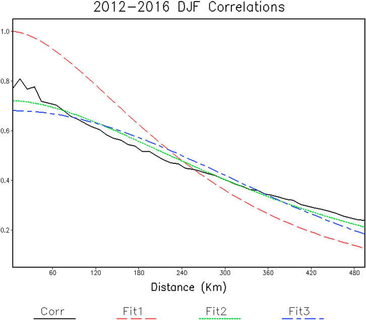
FIGURE 2. Snow depth correlations as a function of horizontal separation distance. The observed correlations, Corr, and the indicated model fits are shown.

Model fits of horizontal correlations are also shown, and the fitted parameters are listed in Table 1. Because it does not have an amplitude parameter, Fit1 has the largest root-mean-square error (RMSE) compared to the measured correlations. Fit1 also has a shorter effective e-folding scale than the others: about 296 km compared to 430 km and 431 km for Fit2 and Fit3, respectively. The Fit2 function is similar to the Fit1 function, but because it includes an amplitude estimate it gives a much better fit. The Gaussian equation, Fit3, also gives a good representation of the measured correlations with an effective e-folding scale and RMSE similar to Fit2. The results discussed here suggest that snow depth data over a large horizontal distance may be used to influence snow depth interpolation to a point.

TABLE 1

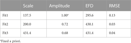
TABLE 1. The scale parameter (${\alpha }^{-1}$), amplitude (A), effective e-folding distance (EFD), and root-mean-square error (RSME) for three fits to horizontal snow-depth correlations. All units are in km except for the dimensionless amplitude.

The Fit1 estimate is distorted by its requirement to approach 1, as the lag distance approaches 0. Both Fit2 and Fit3 give estimates of the amplitude at roughly 0.7. As discussed by Thiébaux and Pedder (1987), the amplitude can be used to estimate the noise/signal variance ratio by

${ϵ}^2=\frac{1-A}{A}.(15)$

For Fit2 and Fit3, the noise/signal variance ratio is about 0.43 (i.e., the signal/noise variance >2).

For vertical correlations of snow depth, we found that after bin seven correlations sometimes become negative and values can be erratic. Also, correlations could not be computed for all of the higher bin numbers. This could be from data noise or decorrelation over too large a vertical distance, which, in either case, would suggest that data with that large separation distance are likely not reliable for interpolation. Therefore, we use only the first nine bins in the fits discussed here, giving a vertical range of 900 m.

The vertical correlations are fit to the same three equations and the observed and fit correlations are evaluated (Figure 3). Statistics for the fits are listed in Table 2. Both Fit1 and Fit2 give similar results because the correlation for the first lag-distance bin is close to 1. Fit3 gives a slightly better fit to the vertical correlations. Fit3 is also the fit used by Brasnett (1999) for vertical correlations, with an effective e-folding distance for the analysis snow depth increment of 800 m. However, here the effective vertical e-folding distance for snow depth is substantially smaller, 461 m for Fit3, suggesting more vertical variation in observed snow depth than an analysis increment. For the daily snow depth increment, discussed later, the vertical scale is also larger than that for snow depth. Note that there is also a high estimate signal/noise variance ratio from the snow depth vertical fits.

FIGURE 3

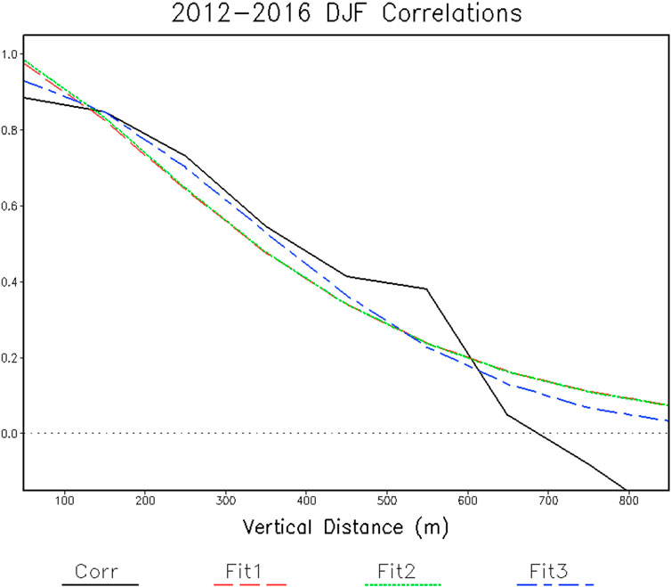
FIGURE 3. Snow depth correlations as a function of vertical separation distance. The observed correlations, Corr, and the indicated model fits are shown.

TABLE 2

TABLE 2. The scale parameter (${\alpha }^{-1}$), amplitude A), effective e-folding distance (EFD), and root-mean-square error (RSME) for three fits to vertical snow depth correlations. All units are in m except for the dimensionless amplitude.

3.2 Daily snow depth increment correlations

For horizontal daily snow depth increment statistics, Fit1 is clearly inferior to the others (Figure 4), because of the amplitude constraint. The amplitude is lower than the amplitude for snow depth because daily changes include noise from the previous day and the day of interest (Table 3). Since the noise at both times is independent the daily change noise variance is about twice the noise variance of snow depth. From Equation 15 and Table 1 the snow depth noise variance is estimated to be about 0.4, while using Table 3 values the daily snow depth increment noise variance is estimated to be close to 0.9. Often the length scale for daily increments is larger than for the full data, but for snow depth the horizontal scales are slightly smaller for the daily increments. This suggests that day-to-day changes can be large and inconsistent between locations with large horizontal separation distances. However, the fitted horizontal e-folding scales for daily snow depth increments are still large, 366 and 378 km for Fit2 and Fit3, respectively (Table 3), suggesting that both snow depth and the daily increments over a large horizontal distance may be used for interpolation.

FIGURE 4

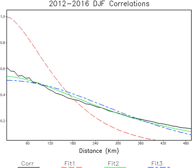
FIGURE 4. Daily snow depth increment correlations as a function of horizontal separation distance. The observed correlations, Corr, and the indicated model fits are shown.

TABLE 3

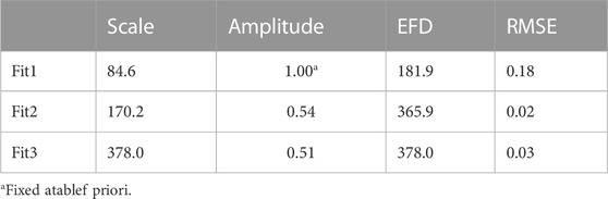
TABLE 3. The scale parameter (${\alpha }^{-1}$), amplitude A), effective e-folding distance (EFD), and root-mean-square error (RSME) for three fits to horizontal daily snow depth increment correlations. All units are km except for the dimensionless amplitude.

For vertical separations (Figure 5) the fits are also better using Fit2 and Fit3 because of the amplitude parameter. The vertical scale for the daily snow depth increment is much larger than for snow depth, 1,167 m (Table 4) versus 461 m (Table 2) for Fit3, indicating relatively little day-to-day snow depth variations over large vertical separations. However, the noise variance for the vertical daily variations is much larger than for vertical snow depth. Some of that greater noise may reflect day-to-day differences in blowing snow, snow sliding down mountain sides, or melting at different mountain locations. The larger vertical scales in daily variations suggest that most of the time there is day-to-day stability between different altitudes, while the much larger noise suggests that there can be events that cause large changes. Note also that the Brasnett (1999) snow depth increment vertical scale (800 m) is larger than that of the observed snow depth (461 m) estimated from our study. These results suggest that over mountain terrain analysis of the increments may be better than the interpolation of snow depth data.

FIGURE 5

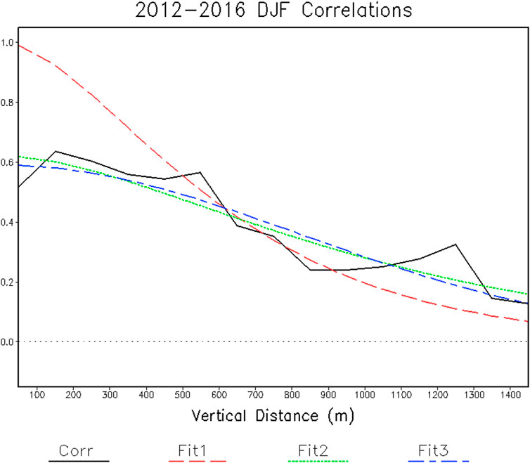
FIGURE 5. Daily snow depth increment correlations as a function of vertical separation distance. The observed correlations, Corr, and the indicated model fits are shown.

TABLE 4

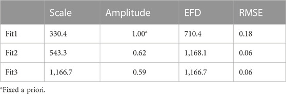
TABLE 4. The scale parameter (${\alpha }^{-1}$), amplitude A), effective e-folding distance (EFD), and root-mean-square error (RSME) for three fits to vertical daily snow depth increment correlations. All units are m except for the dimensionless amplitude.

3.3 Assumptions and their impact on the results

The aim of the study was to estimate regional horizontal and vertical correlation scales from snow depth observations over North America for use in Kriging/OI. Scales were assumed to be fixed parameters over the selected region and are considered for the winter period only. The study showed that these assumptions are reasonable using snow depth data from GHCN-Daily. The distinct pattern of lag correlations of observations over the selected region is indicative of the large scale structure of snow depth spatial variability. The exponential correlation functions of horizontal distance and elevation used in operational snow depth analysis were found to be a good fit to the observed lag correlations.

It was necessary to perform two separate analyses: an analysis over the eastern regions with relatively flat topography to estimate horizontal scales and over the western regions characterized by high mountain terrain to estimate vertical scales. Fitting observed correlations using horizontal distance and elevation as predictors simultaneously is a valid method—a correlation function such as this can be used for interpolation - but the data are not dense enough for simultaneous estimation of horizontal and vertical scales. Using these data errors can occur in situations where horizontal correlations are estimated over mountain environments without considering elevation. Our study found a large effect of elevation on observed snow depth correlations over the high mountain regions of North America: On average, the observed snow-depth correlation e-folding vertical distance is 461 m. Therefore, horizontal correlation scales estimated over areas with steep elevation gradients could be severely underestimated.

The amplitude is a useful parameter for Kriging/OI. An amplitude smaller than one indicates noise in the data. The noise variance is computed from the amplitude via Eq. 15 and when incorporated, it can lower the weight of local observations in the analysis because of their noise. This can result in a smoother interpolation. If noise is not considered, then the analysis may indicate artificial variations caused by noise rather than by signal.

The horizontal amplitude estimate over the eastern regions is about 0.7, indicating a signal/noise variance of about 2 (Eq. 15). The amplitude estimate for vertical distance correlations over the western regions was found to be close to 1, indicating a much higher signal/noise variance. With perfect data and full sampling, the two amplitudes should be the same, since in theory they are a function of the noise/signal variance ratio for the same data. In practice, the amount of sampling and the compromises necessary to make practical computations causes differences. Using the smaller estimate is recommended both because it is based on more data over a larger area, and because it represents a higher level of noise and is therefore less likely to allow noise to contaminate the analysis. The study found a smaller amplitude, about 0.5–0.6 for the daily snow depth increments, yielding a signal/noise variance ratio of about 1. This means that more daily increment observations are needed to reduce the noise and to produce more spatially detailed interpolations of increments. However, use of the daily increments especially over mountain environments can potentially produce a better analysis than that of full snow depth even in the presence of a higher level of noise because of the large correlation scales of the increments and incorporation of temporal information into the analysis.

For horizontal correlations of both full snow depth and daily increments, the horizontal length scales are an order of magnitude larger than the spatial grid scale of 10 km. Thus, sub-grid scale variability should have negligible influence on the measured large scale structure. However, the binned vertical correlations and the vertical scale estimates are less certain due to lower sampling available for their estimates. The data are not sufficient for resolving vertical scales less than the bin width of 100 m, and the vertical statistics should be thought of as a rougher estimate than the horizontal statistics. Because of the limited sampling, we used the data available to compute only one set of statistics and scale parameters for the region. Exploration of spatially and seasonally adjusted correlation scales was also considered initially but was abandoned because of the uneven sampling density. Future studies using better data and methods may be able to improve correlation statistics, especially for regions with large changes in elevation.

4 Conclusion

Measurements of horizontal and vertical DJF snow depth and daily snow depth increment correlation scales over a densely-sampled part of North America are estimated from the fit to exponential equations used to represent correlations of analysis snow depth increments.

The results of our evaluation indicate large horizontal correlation scales for measured snow depth and the daily snow depth increments estimated at about 430 km and 370 km, respectively, when the fit to equations includes an amplitude estimate, which is generally less than 1. These large horizontal scales indicate that in regions with limited topography snow depth and its daily variations may be better analyzed using data with greater horizontal separation. The horizontal Gaussian estimate of correlation (Fit3) gives estimates comparable to that of autoregressive function (Fit2).

Correlations due to vertical separation distances are harder to measure due to lower sampling over mountainous regions. However, we showed here that vertical correlation equations can be fit to data from stations with minimal horizontal separation. All the three fits to vertical correlations are similar, although the Gaussian estimate (Fit3) is slightly better. The measured and fitted vertical correlation scales for snow depth and much smaller than for daily snow depth increments suggesting that analysis based on interpolation of snow depth in regions with large topographic changes requires more data to maintain the same accuracy. It may be possible to use a satellite-based proxy, tuned and bias adjusted against in situ data, to aid analysis in mountainous regions when using snow depth. Without additional data, the analysis will have larger uncertainty in those regions. The Brasnett (1999) vertical correlation scale for snow depth analysis increments of 800 m is also larger than the vertical scale of observed snow depth of 461 m. This suggests that over regions with large changes in elevation analysis of the increments may give better results with sparse data. Analysis of the daily increments from the analysis for the previous day can be useful since it has large scales, especially the vertical scale, and because it includes temporal information. Some testing may be needed to show which type of analysis is best for a given application.

Estimating the amplitude reduces the fitting errors, avoids overestimation of the correlation at short separation distances, and allows estimation of the noise/signal variance ratio for use in optimal interpolation.

Our results indicate potential utility for operational snow analysis. For example, the persistence of large horizontal scales of observations and the daily increments in the scenarios considered imply that horizontal increment analysis scales larger than 120 km can be tested for improved predictions especially over remote areas, or assessments such as this can be performed to estimate scales for a specific analysis application.

Data availability statement

The raw data supporting the conclusions of this article will be made available by the authors, without undue reservation.

Author contributions

CK and TS wrote the initial draft of the paper and provided equal contributions. All authors contributed to the writing—review and editing of the final written version.

Funding

This research was funded by NOAA, grant number NA18NWS4680053 and NOAA, grant number NA21OAR4590381.

Conflict of interest

The authors declare that the research was conducted in the absence of any commercial or financial relationships that could be construed as a potential conflict of interest.

Publisher’s note

All claims expressed in this article are solely those of the authors and do not necessarily represent those of their affiliated organizations, or those of the publisher, the editors and the reviewers. Any product that may be evaluated in this article, or claim that may be made by its manufacturer, is not guaranteed or endorsed by the publisher.

References

Brasnett, B. (1999). A global analysis of snow depth for numerical weather prediction. J. Appl. Meteor. 38, 726–740.

CrossRef Full Text | Google Scholar

Brown, R. D., Brasnett, B., and Robison, D. (2003). Gridded North American monthly snow depth and snow water equivalent for GCM evaluation. Atmosphere-Ocean 41, 1–14. doi:10.3137/ao.410101

CrossRef Full Text | Google Scholar

Daley, R. (1991). Atmospheric data analysis. Cambridge: Cambridge University Press, 457.

Google Scholar

de Rosnay, P., Balsamo, G., Albergel, C., Muñoz-Sabater, J., and Isaksen, L. (2012). Initialisation of land surface variables for numerical weather prediction. Surv. Geophys. 35, 607–621. doi:10.1007/s10712-012-9207-x

CrossRef Full Text | Google Scholar

Durre, I., Penne, M. J., Gleason, B. E., Houston, T. G., and Vose, R. S. (2010). Comprehensive automated quality assurance of daily surface observations. J. Appl. Meteorology Climatol. 49, 1615–1633. doi:10.1175/2010jamc2375.1

CrossRef Full Text | Google Scholar

Durre, I., Penne, M. J., and Vose, R. S. (2008). Strategies for evaluating quality assurance procedures. J. Appl. Meteorology Climatol. 47, 1785–1791. doi:10.1175/2007JAMC1706.1

CrossRef Full Text | Google Scholar

Gan, Y., Zhang, Y., Kongoli, C., Grassotti, C., Yong, Y-K., Liu, Y., et al. (2021). Evaluation and blending of ATMS and AMSR2 snow water equivalent retrievals over the conterminous United States. Remote Sens. Environ. 254, 112280. doi:10.1016/j.rse.2020.112280

CrossRef Full Text | Google Scholar

Jaffrés, J. B. D. (2019). GHCN-daily: A treasure trove of climate data awaiting discovery. Comput. Geosciences 122, 35–44. doi:10.1016/j.cageo.2018.07.003

CrossRef Full Text | Google Scholar

Japan Meteorological Agency (JMA) (2019). Outline of the operational weather numerical prediction at the Japan Meteorological Agency. Appendix to WMO Technical Progress Report on the Global Data-processing and Forecasting System (GDPFS) and Numerical Weather Prediction (NWP) Research, JMA, March 2019, Available at: https://www.jma.go.jp/jma/jma-eng/jma-center/nwp/outline2019-nwp/pdf/outline2019_02.pdf

Google Scholar

Kongoli, C., Key, J., and Smith, T. (2019). Mapping of snow depth by blending in-situ and satellite data using two dimensional optimal interpolation – application to AMSR2. Remote Sens. 11 (24), 3049. doi:10.3390/rs11243049

CrossRef Full Text | Google Scholar

Liu, Y., Peters-Lidard, C. D., Kumar, S. V., Arsenault, K. R., and Mocko, D. M. (2015). Blending satellite-based snow depth products with in situ observations for streamflow predictions in the Upper Colorado River Basin. Water Resour. Res. 51, 1182–1202. doi:10.1002/2014WR016606

CrossRef Full Text | Google Scholar

Menne, M. J. I. Durre, Vose, R. S., Gleason, B. E., and Houston, T. G. (2012). An overview of the global historical Climatology network-daily database. J. Atmos. Ocean. Technol. 29 (7), 897–910. doi:10.1175/JTECH-D-11-00103.1

CrossRef Full Text | Google Scholar

Reynolds, R. W., and Smith, T. M. (1994). Improved global sea surface temperature analyses using optimum interpolation. J. Clim. 7, 929–948. doi:10.1175/1520-0442(1994)007<0929:igssta>2.0.co;2

CrossRef Full Text | Google Scholar

Thiébaux, H. J., and Pedder, M. A. (1987). Spatial objective analysis with applications in atmospheric science. Cambridge: Academic Press, 299

Google Scholar

Thiébaux, H. J. (1985). On approximations to geopotential and wind-field correlation structures. Tellus 37A, 126–131. doi:10.3402/tellusa.v37i2.11660

CrossRef Full Text | Google Scholar

Webster, R., and Oliver, M. A. (2007). Geostatistics for environmental scientists, Second Edition. England: John Wiley & Sons, 315.

Google Scholar