 Hongwu Lei
 Yingchun Xie2
- 1State Key Laboratory of Geomechanics and Geotechnical Engineering, Institute of Rock and Soil Mechanics, Chinese Academy of Sciences, Wuhan, China
- 2CNNP Kunhua Energy Development Co. Ltd, Hangzhou, China
- 3No.280 Research Institute of Nuclear Industry, Guanghan, China
Two-phase flow (flow of water in both liquid and gas phase, containing a non-condensable gas such as CO2) in the wellbore is one of the most important processes in the production performance and wellbore scaling evaluations of high temperature geothermal wells. This paper first describes the discharge tests in the Yangbajing geothermal field, Tibet. Next, a simple model for governing the two-phase flow in the presence of CO2 in the wellbore is constructed and a robust calculation method is presented. The model is applied to three production wells in the Yangbajing geothermal field. The results show that the velocity difference between the gas and liquid phase should be included in the model. Ignoring this difference (i.e., homogeneous model) would result in a significant deviation between measurements and calculations. A drift flux model (DFM) describes the velocity difference, where the specifics of the particular model can have significant effects on the results for the pressure and temperature profiles in the wellbore. Three commonly used DFMs are compared to estimate their performance. The calculated wellhead pressure and temperature are in the range of 2,3 bar and 125°C–135°C for all three wells at a production rate of about 20 kg/s. The estimated wellhead gas mass fraction is between 3% and 8%. Considering CO2 content, three different scenarios were evaluated, although the effect on the pressure and temperature profiles were limited. However, CO2 content has a much more significant effect on the flash depth, which is an important parameter for the estimation of calcite scaling.
1 Introduction
As a natural resource with low carbon content and huge reserves, geothermal energy has become a promising renewable energy source and has started to attracted more attention. Theoretical calculations show that the energy reserves in the upper 10 km of the Earth’s crust are approximately 3.6 ✕ 1014 GWh (Lund et al., 2008), about 2.17 million times the global energy consumption of 2012. There are roughly 88 countries (regions) making use of geothermal energy directly (Lund and Toth, 2021), and more than 30 countries (regions) using geothermal energy for power generation (Huttrer, 2021). Most of the geothermal energy is used by geothermal heat pumps. About 12.9% is used for electricity generation (Lund et al., 2022), accounting for just 0.3% of the total power generation and 1.5% of the power generated from renewables (Zhu et al., 2015). The United States is the leading country in geothermal applications. It has the largest installed capacity of geothermal power production, reaching 28.8% of the total geothermal power production. Additionally, it has the second largest installed capacity of direct geothermal utilization. China is number one when it comes to direct geothermal utilization, reaching 25.2% of the total. However, the installed capacity of geothermal power generation is only 27.28 MWe, accounting for just 0.2% of the total geothermal power production and ranking 18th in the world (China Geological Survey of Natural Resources Ministry et al., 2018).
China has rich geothermal resources, with a value of 3.06 ✕ 1018 kWh/a accounting for 7.9% of the total global geothermal energy reserves (Jiang, 2012). However, the distribution of geothermal resources is uneven but with obvious regularity and regionality. At present, a basic primary pattern for geothermal energy utilization in China has been formed (Zhu et al., 2015). Yangbajing in Tibet features geothermal power generation. Geothermal heating is widely used in Tianjin, Xi’an and Beijing. Groundwater and sea water source heat pumps for heating and cooling are widely used in Chongqing and Dalian. The coastal regions in South and East China are popular for recuperation and tourism related utilization such as spa hotels and hot spring resorts. The first high-temperature geothermal power generation station in China was built in Yangbajing, Tibet in 1977. The total installed capacity is currently 26.18 MW. In the past few decades, the power station has contributed 50% of Lhasa’s summer power supply and 60% of winter power supply (Zhang et al., 2019). However, the operation of the power station was suspended due to the low power generation efficiency, poor economic efficiency (Zhang et al., 2019), geothermal wastewater (Guo and Wang, 2009) and scaling problems (Zhou, 2003).
The wellbore is the only conduit available to extract geothermal fluid from reservoirs. Some important physical and geochemical processes such as phase change, gas exsolution and mineral precipitation are likely to occur as a result of the fluid flowing upward, and these processes can significantly affect the production performance of a wellbore. Two-phase flow with phase change is generally the basis for another processes in wellbores. Due to the difficulty in measuring directly some important parameters as the harsh operating conditions in geothermal wellbores prevent the installation of measuring equipment. Therefore, wellbore flow simulator is an invaluable tool for obtaining the information on flow behavior.
Barelli et al. (1982) constructed a model that simulates a two-phase flow in geothermal wells that contain CO2, and gives an estimate of temperature and pressure profiles which are then compared to measurements of the specific well. Bjornsson et al. (1993) developed the geothermal wellbore simulator HOLA. The simulator can reproduce the measured flowing temperature and pressure profiles in flowing wells and determines the relative contribution of each feed zone for a given discharge condition. Pan and Oldenburg. (2014) originally developed the simulator T2Well in the TOUGH2 framework to model two-phase flows in coupled wellbore-reservoir systems. Vasini et al. (2018) plugged EWASG (Battistelli et al., 1997) into T2Well in order to extend the functionality of computing two-phase flow for high enthalpy geothermal systems. The module EWASG can consider fluids containing dissolved solids and one non-condensable gas (NCG) such as CO2, CH4, H2S, H2 or N2. Gunn and Freeston. (1991) developed an integrated geothermal wellbore simulator called WELLSIM, which can perform calculations including discharge tests, fluid composition and properties, deliverability curve prediction, statistical and graphical matching analysis of downhole pressure and temperatures and downhole measurement analysis. Hasan and Kabir. (2010) presented a robust model for a two-phase flow in geothermal wells using the drift-flux approach. Deendarlianto and Itoi. (2021) constructed a wellbore model to numerically investigate the effects of CO2 gas on the two-phase flow characteristics in geothermal production wells. Lei et al. (2022) evaluated the two-phase flow in the geothermal wells by the Shi et al. (2005) model. Li et al. (2020) used HOLA and WELLSIM to simulate the two-phase flow of a high temperature geothermal well in the Kangding geothermal field for quantitative assessment of calcite scaling. Recently, Tonkin et al. (2021) reviewed geothermal wellbore models and compared their differences and effects on simulations. Furthermore, Canbaz et al. (2022) performed a comprehensive literature review of studies about wellbore dynamics involving geothermal fluids’ physical and thermodynamic behavior during production and injection in the presence of CO2 along the wellbore.
This paper aims to estimate the two-phase flow and related production performance in the Yangbajing geothermal field by comparing numerical simulation with those obtained from discharge testing. It is organized as follows: Section 2 briefly introduces the field condition, and pressure and temperature measurements during discharge testing. Section 3 describes the details of the wellbore model. In Sections 4 and 5 the proposed wellbore model is used to simulate the two-phase flow of typical production wells in the Yangbajing geothermal field. Finally, the main observations and conclusions are summarized in Section 6.
2 Study area
2.1 Geological settings
The Yangbajing geothermal field is located in a fault basin of the Nyainqentanglha range, about 90 km northwest of Lhasa, at an elevation of 4,290–4,500 m with a high altitude in the northwest and a low altitude in the southeast. There are strong tectonic activities in the geothermal field, with three groups of faults developing in northeast, northwest and north-south directions. The China-Nepal highway divides the field into two parts, the southern and northern. The south area is composed of porous Quaternary strata, while the north area is composed of a combination of porous Quaternary strata and Himalayan fractured granite (Duo, 2003).
The thermal groundwater system consists of two reservoirs at different depths. The shallow geothermal reservoir is located 180–280 m below the surface, and the lithology is composed of Quaternary alluvial sandy gravel layers, moraine gravel and weathered granite crust on top of the bedrock. The cap rock of the geothermal reservoir is composed of muddy gravel or silty clay layers with varying thickness. The bedrock at the bottom of the geothermal reservoir is composed of early Himalayan granite and tuff, and mylonite granite is found locally in the northern part of the geothermal field (Duo, 2003; Guo et al., 2007).
According to the magnetotelluric exploration results, there is a low resistance layer with a resistivity of 5 Ω m at a depth of 5 km in the northern part of the Yangbajing geothermal field, which is inferred to be a cooling magma chamber and the heat source of the geothermal field (Chen, et al., 1996; Duo, 2003). A fault fracture zone is present in the piedmont of the north, with a local width of about 1 km. The shallow normal faults are connected with the deep strike-slip faults, effectively connecting the deep heat source and the shallow reservoir. The results of analysis of the hydrogen and oxygen isotopes of the groundwater in the thermal field (Guo et al., 2010) indicates that the subterranean hot water in this area is the result of a large amount of melt water from the Nyainqentanglha Mountain flowing into the ground along the fault zone, circulating deep, and being heated by the deep magma heat source (Duo, 2003) (Figure 1).
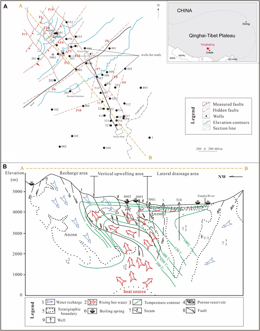
FIGURE 1. The location and geological profile of the study area:(A) plan, (B)cross section (Modified from Duo, 2003; Xu et al., 2018).
The fluid is mainly in liquid state containing a little gas. Guo. (2012) reviewed the hydrogeochemistry of the Yangbajing geothermal field, indicating that 1) the TDS of the hot fluid is about 1,266 mg/L and Na+, Cl− and HCO3- are the dominant ions, and 2) CO2 originated from the metamorphism of the Nyenchen Tonglha core complex is a major component of geothermal gases. Gas sampling by a separator at the wellhead was carried out by Zhao et al. (1998). The results showed that CO2 content in the gas-phase was between 21.4 and 66.10 mmol/kg. CO2 was the dominant composition of non-condensable gas (Table 1).
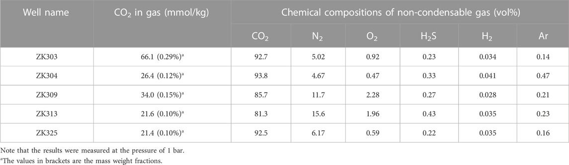
TABLE 1. Wellhead gas composition (Zhao et al., 1998).
The geological survey in the Yangbajing geothermal field began in 1976. During the exploration stage, 45 exploration wells were drilled and a thermal field with an area of 42 km2 was delineated. In the 1980s, another 25 production wells and 13 recharge wells were successively drilled. Since September 1977, the first 1 MW test unit has successfully been generating power. The power generation capacity had been expanded to 25.18 MW by 1991. By the end of 2017, the field consisted of four production wells in the south, 12 production wells in the north, and five recharge wells, reaching a total installed capacity of 24.18 MW and a cumulative power generation of more than 33×108 kW h. The fluid production rate was about 12,000 t/d in the peak production period. The initial fluid temperature of most production wells was 125°C–145 °C, with a pressure of 1.76–3.72 bar. The temperature in the shallow geothermal reservoir is ranging from 140°C to 160°C. The pressure in the reservoir varies from about 0.8 MPa to 3.0 MPa, depending on the depth. However, the pressure and temperature of the production wells showed a decreasing trend with time before 2012. Pressure and temperature were gradually restored after recharge normalization after 2012 (Xu et al., 2018). The long-term fluid extraction leaded to considerable surface subsidence around the geothermal fields (Li et al., 2015).
2.2 Discharge testing
In order to analyze the flow of the wellbore, the discharge testing was carried out from April to May 2020 in three typical wells, namely, ZK303, ZK324, and ZK304. The ZK303 well has a depth of 300 m, where the first 142.5 m in depth is in the Quaternary layer. Below 142.5m, the well extends into the fractured layer. The maximum depth of mechanical descaling of this well is about 150 m, and the scaling occurs above ∼80 m (Figure 2A). The ZK324 well has a depth of 90.13m, and the entire well section is in the Quaternary sandy gravel layer. The maximum depth of mechanical descaling of this well is about 86 m, and the scaling occurs above ∼70 m (Figure 2B). The ZK304 well has a depth of 206.54 m, with the Quaternary porous layer from 0 m to 142 m in depth and the fractured layer below the depth 142 m. The maximum depth of mechanical descaling is 117.17 m, and the scaling occurs between 80 m and 130 m (Figure 2C).
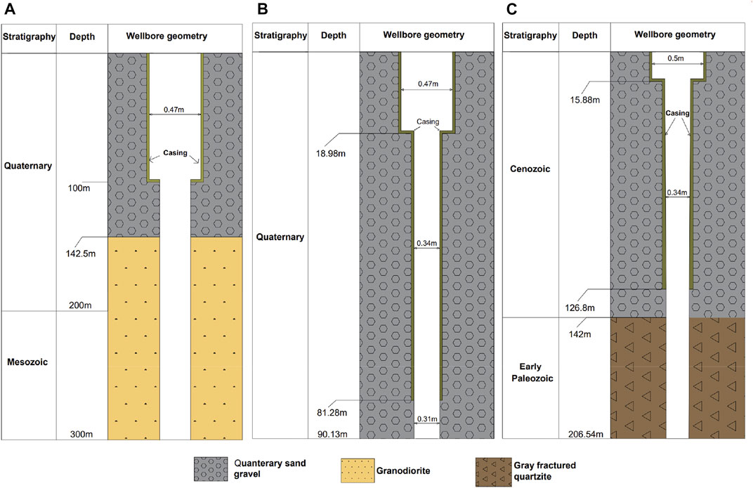
FIGURE 2. Wellbore structure of the test wells, (A) ZK303, (B) ZK324, (C) ZK304.
The James lip pressure method was adopted in the discharge testing, using the Kuster K10 PT Geothermal Instrument as the main test tool. Discharge stimulation was conducted after the static PT test (i.e., without discharge) and a continuous PT test was performed from the bottom to the top with wellhead fluid discharge. The flow rate was measured at the wellhead. Figure 3 shows the test results. It can be seen that the temperature and pressure at the bottom of the well are not much different under the two testing conditions, but the difference at the upper part of the wells is relatively large. In the static state, the water level is below the wellhead elevation; the water levels of ZK303 and ZK304 are at the depth of 50–60 m, and the water level of ZK324 is at the depth of about 10 m. Due to the combined effects of atmospheric environment, geothermal reservoirs and surrounding rocks near the wellbore, the temperature shows a large gradient. In the dynamic state, the wellhead temperature is relatively low due to the influence of atmospheric environment, but the temperature at the depth of 10 m is 118°C–135°C.
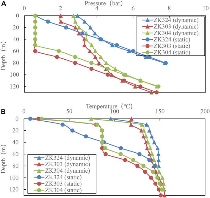
FIGURE 3. Temperature and pressure test results, (A) pressure, (B) temperature.
To further analyze the phase characteristics from the downhole to the wellhead under dynamic condition, the data of temperature and pressure are plotted on the water phase diagram. It can be seen from Figure 4 that the fluid in the three wells is in a single liquid-phase state at the bottom. As the fluid flows upward, the pressure gradually decreases and the fluid begins to evaporate when it drops to the saturation pressure of the corresponding temperature. As a result, the temperature decreases and the system goes to two-phase state. In the two-phase state, the relationship between temperature and pressure is locked by the water saturation line. Due to the influence of the surface environment, ZK324 and ZK304 experienced strong condensation at the wellhead during the testing, which caused the fluid state to return to single liquid-phase.
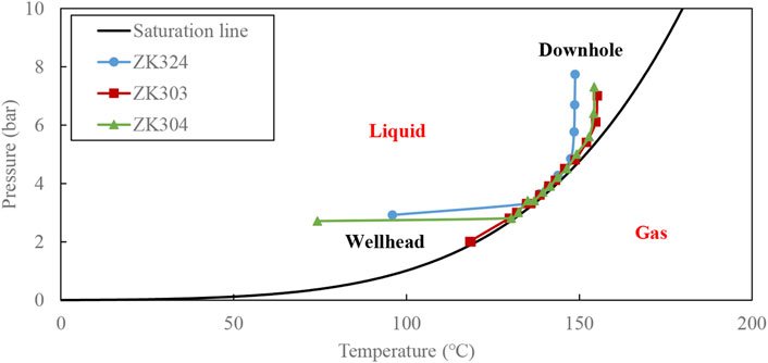
FIGURE 4. Phase behavior along wellbore under dynamic test condition.
The phase diagram (Figure 4) shows that the change in pressure and temperature is almost along the path of the saturation line of pure water. It indicates that CO2 in the system is limited. The measurements of wellhead steam compositions (Zhao et al., 1998) showed that the CO2 mass weight fractions in steams are 0.29% and 0.12% for ZK303 and ZK304, respectively. Furthermore, a large amount of calcite scaling was found in the wellbore during several years of operation (Zhou, 2003), which is strongly associated with the presence of CO2. Therefore, the presence of CO2 should be considered in the evaluation of two-phase flow.
3 Simulation method
3.1 Flow with phase change in one-dimension wellbores
The components of fluid in the Yangbajing geothermal fields contain H2O and CO2 and phase change may occur when the fluid flows upward in the wellbore. Based on mass, momentum and energy conservations, a one-dimensional non-isothermal flow model with phase change can be constructed for the wellbore. Assuming steady state and uniform distribution of variables (i.e., temperature, pressure, gas-phase fraction, density and velocity) along the wellbore cross-section and ignoring the axial heat conduction of the fluid in the wellbore, the equations can be described by the following form (Tonkin et al., 2021)
where.
-
-
-
-
-
-
-
-
-
-
-
-
-
-
-
With the assumption that momentum related terms in Eqs 3, 4 are negligible, and by considering the boundary conditions at the downhole, Eqs 1-4 can be reduced to
The mass rate
Although the uneven distribution of gas bubble would result in the non-equilibrium of CO2 between the gas and liquid phase, this paper also assumes that the component of CO2 has enough chance to reach an equilibrium state between the two phases. According to Henry’s law, the relation between the partial pressure of CO2 and CO2 mass fraction in liquid phase can be expressed as
where
where
The void fraction
For a heterogeneous mixture (i.e.,
where the volumetric flux
3.2 Drift flux model
The parameters of
3.2.1 Rouhani and Axelsson model
A comparison of void fraction correlations based on an unbiased data set showed that the Rouhani and Axelsson. (1970) model had a good fitting result (Woldesemayat and Ghajar, 2007). It is expressed as
where σ is the surface tension between gas and liquid phase.
3.2.2 Hibiki and Ishii model
The pipe diameter has important effect on flow pattern. In a large diameter pipe, slug bubbles cannot be sustained. Due to the interfacial instability, slug bubbles in such flows will disintegrate to cap bubbles. For a large diameter pipe, Hibiki and Ishii. (2003) developed and recommended the parameters as
3.2.3 Shi et al. model
Based on experimental data in a 15-cm-diameter, 11-m-long plexiglass pipe, Shi et al. (2005) determined drift-flux parameters by using an optimization technique that minimizes the difference between experimental and model predictions. The model is written as
where.
-
-η is a parameter reflecting the effects of the flow status on the profile parameters, defined as
-
-
3.3 Flowchart of calculation
A rigorous numerical approach to solve Eqs 1, 2; Eqs 3, 4 includes generating a mesh of the wellbore, establishing the discrete equations, and solving them by the Newton-Raphson iterative method, which was implemented in the T2Well simulator (Pan and Oldenburg, 2014). However, this method has two drawbacks. The first is that the initial conditions for the two-phase flow are very difficult to determine and different initial conditions could result in wildly different results. The second is the lack of robustness of the method; iterative convergence failure is often encountered in the phase change region. Following the method proposed by Barelli et al. (1982), an improved method is demonstrated in Figure 5. This method is based on the fact that the temperature decreases and gas phase fraction increases from the downhole to the wellhead. There are two loops in the calculation, one for temperature, the other for gas phase fraction. For a given temperature decrease, the first loop aims to find the change in the z value. The second loop aims to find the change in the gas-phase fraction.
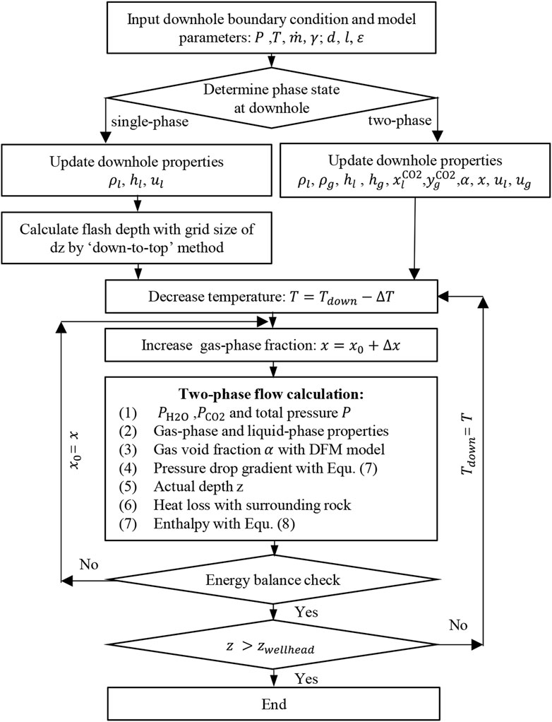
FIGURE 5. Flowchart of calculation.
3.4 Verification
To verify the model, a compared wellbore flow model is taken from Vasini et al. (2018). The downhole CO2 mass fraction is about 3%. Figure 6 shows that the calculations are generally consistent with the measurements and simulation from T2Well-EWASG. The small temperature deviation is due to the reason that the model in this study has ignored the heat exchange with surrounding rock. Compared with T2Well-EWASG, the model is simple and easy to implement.
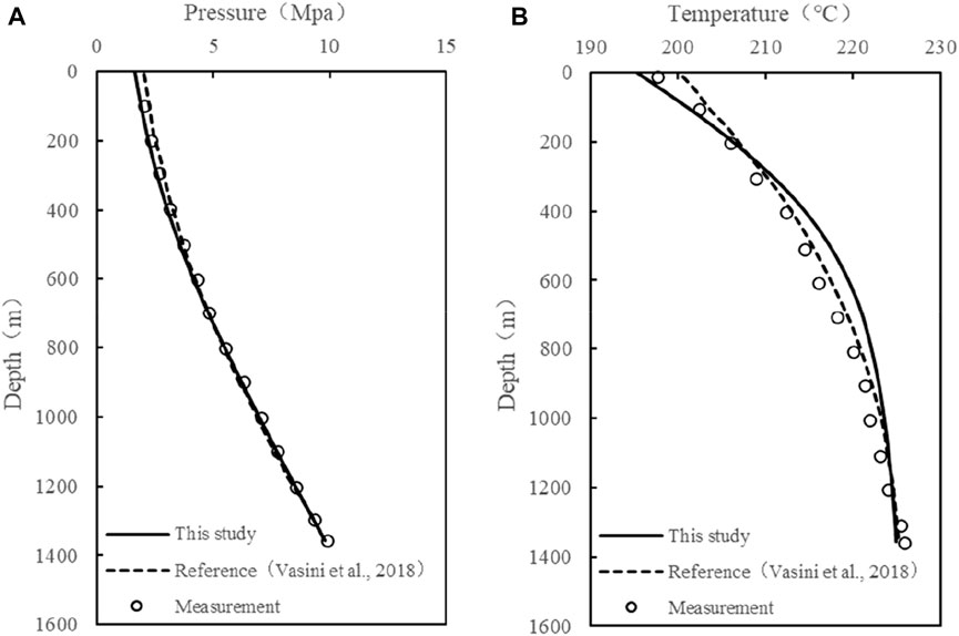
FIGURE 6. Comparison with T2Well-EWASG: (A) pressure and (B) temperature.
4 Model setup
The parameters and boundary conditions for wellbore models are listed in Table 2. Due to the lack of downhole fluid samples during the testing, the key parameter of the CO2 mass fraction at the bottom of casing pipe is unknown. However, according to the previous mechanical descaling, the flash depth of both the three wells is above the casing bottom, which means that the fluid is in single-phase state at the casing bottom. Therefore, it can be calculated by the Henry’s law that the CO2 mass fractions at the bottom of the casing pipe for ZK304, ZK303 and ZK324 cannot be higher than 0.08%, 0.06% and 0.12%, respectively. To account for the uncertainty of CO2 content, three different cases were simulated. In Case 1, the fluid is fully saturated with CO2, In Case 2, the amount of CO2 is half the amount of the fully saturated case and Case 3 has no CO2 present. Because of the large production rate and the short wellbore casing, the heat exchange with the surrounding rock is ignored in the model. The calculation is implemented from the downhole to the wellhead. The grid size for single-phase calculation is set to be 1.0 m, while for two-phase calculation it varies depending on the given temperature decrease in Figure 5. The value of 0.1 or less is suggested.
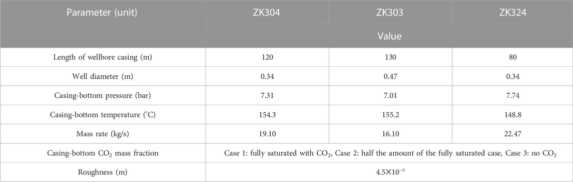
TABLE 2. Parameters for flow models.
5 Results
The results from the aforementioned three drift flux models are compared. Figure 7 shows that there is a noteworthy difference between the measurement and calculation with the homogeneous model for ZK324. The calculation from the Shi et al. model is the closest to the measurement results, with average errors for pressure and temperature of respectively 3.58% and 0.79% (Table 3). The CO2 content has a certain effect on the pressure and temperature profiles; a low CO2 content results in a lower temperature and pressure. The calculated wellhead pressures according to the Shi et al. model are respectively 3.2, 3.1 and 3.0 bar for the three specified scenarios of CO2 content (Case 1, 2 and 3. The corresponding temperatures are 135, 134°C and 133°C, respectively.
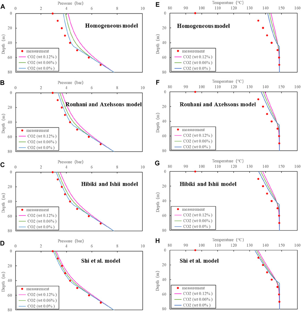
FIGURE 7. Comparison of simulations with different models and measurements for ZK324:(A), (B), (C) and (D) for pressure, (E), (F), (G) and (H) for temperature.
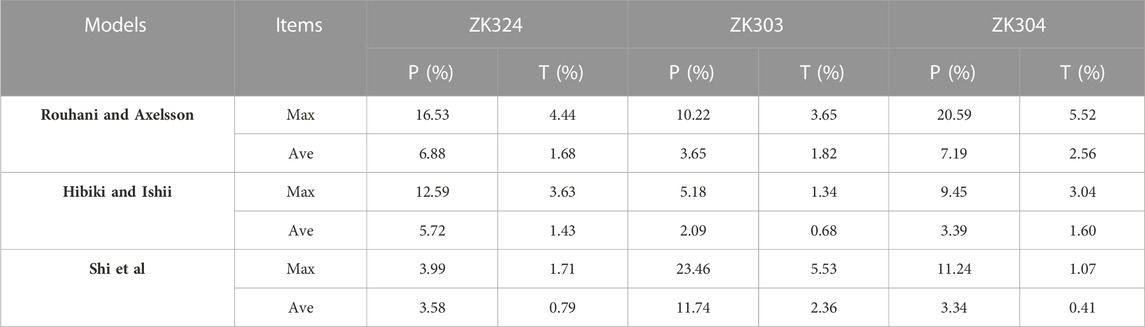
TABLE 3. Errors between the calculations and measurements for different Drift flux models.
From Figure 8, the results of the Hibiki and Ishii model are generally closest to the measurements for ZK303. With average errors for pressure and temperature of respectively 2.09% and 0.68%, (Table 2), it outperforms the Shi et al. model. The reason for this is the fact that the Hibiki and Ishii model is more suitable for large diameter wellbores than the Shi et al. model. The diameter of the ZK303 well is 0.47 m, 1.38 times bigger than the other two wellbores. Due to the low CO2 content, the presence of CO2 has small effect on the pressure and temperature profiles.
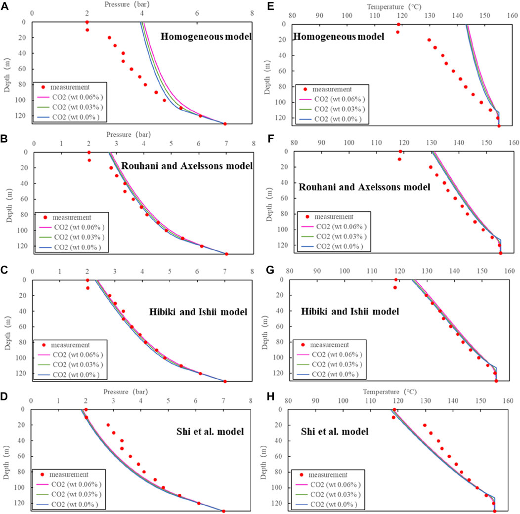
FIGURE 8. Comparison of simulations with different models and measurements for ZK303:(A), (B), (C) and (D) for pressure, (E), (F), (G) and (H) for temperature.
Similar to ZK324, the result from the Shi et al. model show best prediction capability for ZK304 as well (Figure 9). The corresponding average errors for pressure and temperature are 3.34% and 0.41%, respectively (Table 3). Due to the same reason as ZK303, the effect of CO2 content on the profiles of pressure and temperature is ignorable.
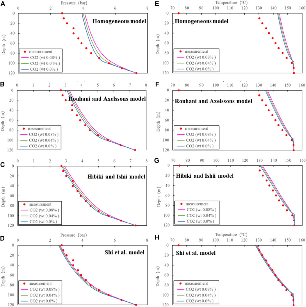
FIGURE 9. Comparison of simulations with different models and measurements for ZK304:(A), (B), (C) and (D) for pressure, (E), (F), (G) and (H) for temperature.
Based on the optimal model (i.e., the best suitable DFM model for fitting), the distribution of another parameter in the wellbore is further analyzed. Figure 10 shows that the flash depth (i.e., the gas void fraction is larger than zero) for ZK324 is about 44.9 m without CO2, while it is 58.1 with 0.06% CO2 (Case 2). The wellhead gas mass fraction is about 0.035 and the corresponding gas void fraction is about 0.75. For the case of 0.06% CO2 content (Case 2), the CO2 mass fraction in the gas phase reaches 0.38 at the flash depth and gradually decreases the next 30 m upwards due to the increase in steam content. The same trend with depth can be observed with the CO2 mass fraction in the liquid phase. Compared with the measured result of CO2 content of averaged 0.15%wt at the wellhead measured by Zhao et al. (1998), the calculation of 1.6% for Case 2 is higher. The reason for this difference is the fact that the measurement was conducted at the pressure of 1 bar, while the calculation was done with a much higher pressure of 3 bar. The decreased pressure results in water transformation from the liquid to gas phase and therefore a low CO2 content was measured. Above the flash depth, the value of the gas void fraction rapidly increases by more than 0.3 and the churn flow pattern (i.e., gas void fraction usually large than 0.25) is dominant.
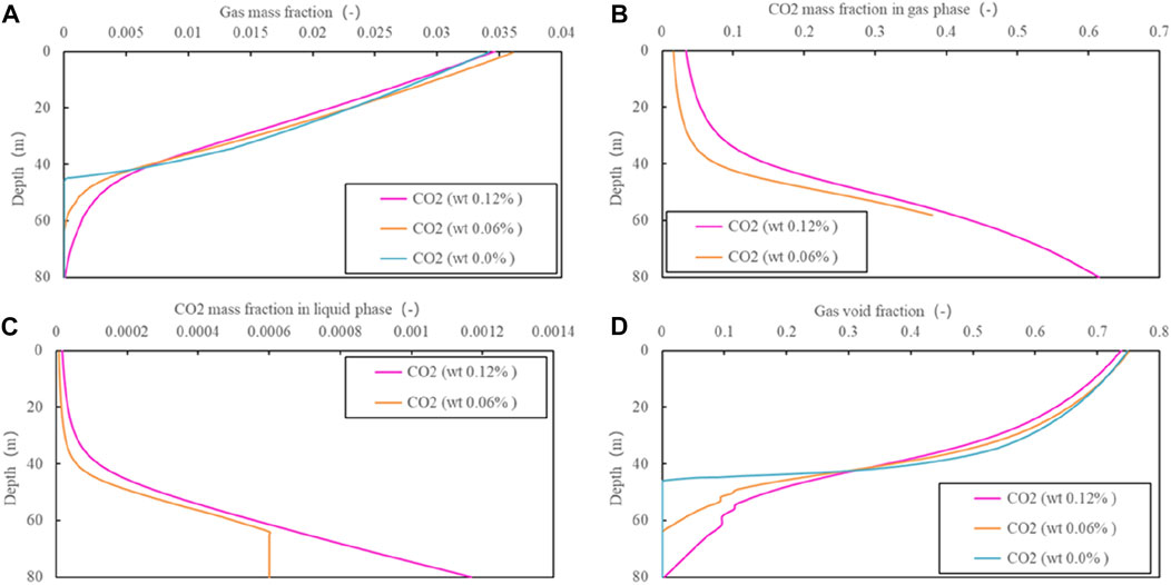
FIGURE 10. Simulated results by Shi et al. model for ZK324.
Figure 11 demonstrates that the flash depth for ZK303 is about 112.5 m without CO2, while it is 119.5 with 0.03% CO2 (Case 2). The wellhead gas mass fraction is about 0.075 and the corresponding gas void fraction is about 0.80. The CO2 mass fraction in the gas phase is about 0.21 at the flash depth for the case of 0.03% CO2. The changes in the CO2 mass fraction in both the liquid and gas phase are small above the depth of 100 m, which indicates that the more severe wellbore scaling mostly occurs between the flash depth and a depth of a 100 m. For the case of 0.03% CO2 (Case 2) in the wellbore of ZK303, the calculated CO2 content of 0.4% is close to the measurement of 0.29% by Zhao et al. (1998).
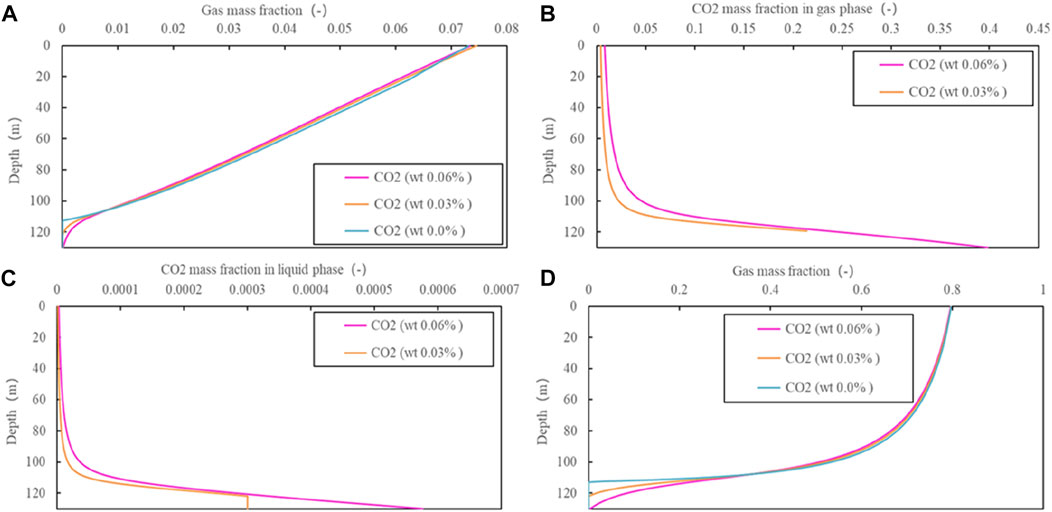
FIGURE 11. Simulated results by Hibiki and Ishii model for ZK303.
Figure 12 indicates that the flash depth for ZK304 is about 97.7 m without CO2 and 107.2 m with 0.04% CO2. The wellhead gas mass fraction is about 0.065 and the corresponding gas void fraction is about 0.84. The maximum CO2 mass fraction in the gas phase for the case of 0.04% CO2 reaches 0.27 at the flash depth. The CO2 mass fractions in both the liquid and gas phase vary dramatically from the flash point down to a depth of 90 m. For the fluid containing half of the CO2 content of the fully saturated case, the calculated wellhead CO2 mass fraction in the gas phase is 0.6%, five times of the measurement of 0.12%. The reason has been explained above.
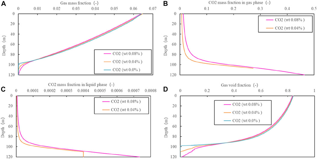
FIGURE 12. Simulated results by Shi et al. model for ZK304.
Comparing the results of the three wells, it can be seen that the proportion of liquid evaporation to steam for the relatively short wellbore length is small and therefore the wellhead temperature is high. The corresponding wellhead pressure is high due to the small pressure loss.
6 Discussions
6.1 Effect of production rate
Based the optimal model, the production performance is analyzed by means of the production rate. It can be seen from Figure 13 that both the wellhead pressure and temperature increase and the gas phase mass fraction decreases with the production rate. With the consideration that the geothermal field will deplete with long-term development due to the decrease in reservoir pressure and wellbore scaling, the production rate is set to half of the testing rate. The results shows that the wellhead temperatures for ZK304, ZK303 and ZK324 decrease by respectively 6.1, 5.4°C and 3.1°C compared to the testing rate. The pressures decrease by 0.44, 0.36 and 0.27 bar, respectively. This is because the change of production rate affects the distribution of two phases and the pressure profile, ultimately affecting the flash process.
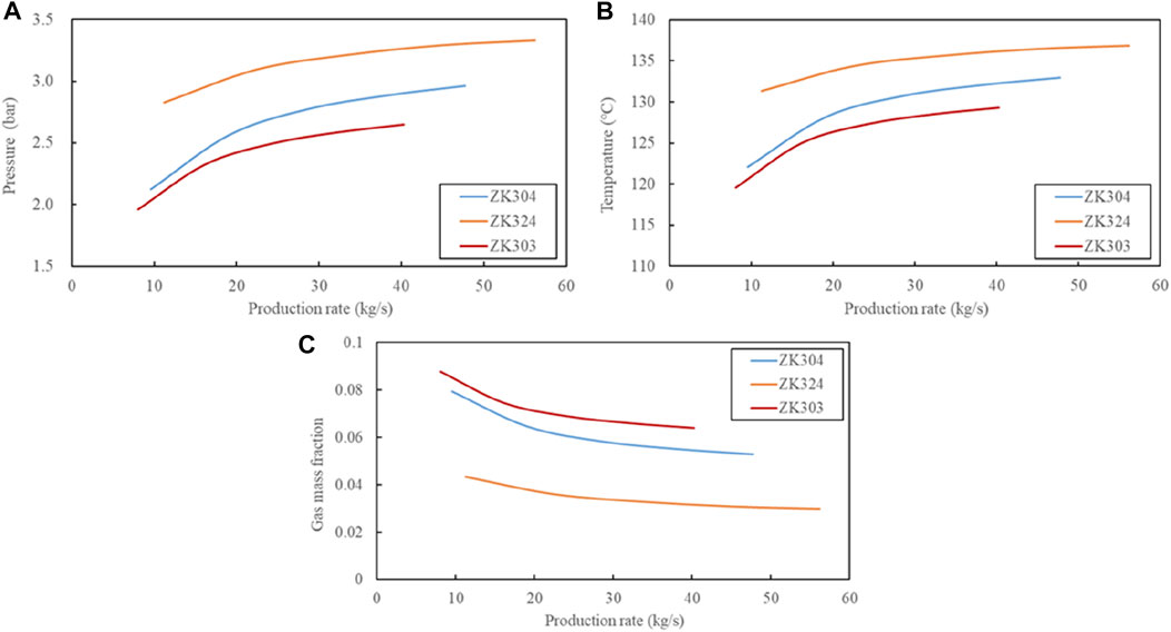
FIGURE 13. Effect of production rate on performance.
6.2 Effect of surrounding rock heat exchange
Giving the parameters
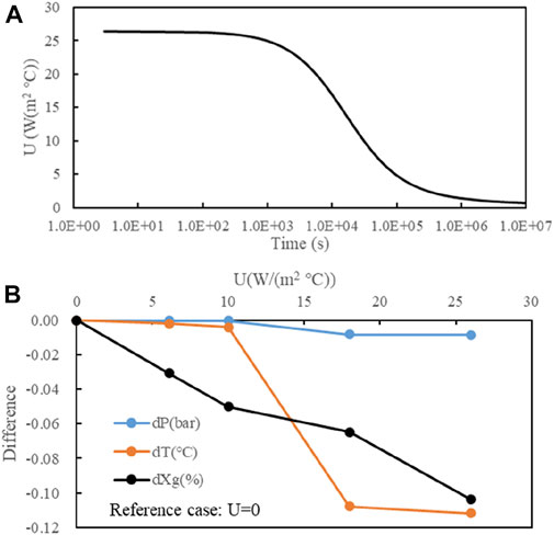
FIGURE 14. Effect of surrounding rock heat exchange based on ZK304: (A) calculated transient heat exchange coefficient, (B) effect on the wellhead performance parameters.
6.3 Effect of calculation parameters
In order to analyze the effect of the calculation parameters such as the grid size and the temperature decrease, the additional two cases (Case 1: based case with dz=1.0, dt=0.1, Case 2: dz=0.5, dt=0.05, Case 3: dz=2, dt=0.2) are used for comparison (Figure 15). The pressure and temperature differences are within 0.2 bar and 2.75 °C, respectively. The maximal difference in gas mass fractions is about 1% at the wellhead. The difference in flash depths is small. This is because that it only determined by the value of dz. Therefore, a small grid size and temperature decrease should be used in the calculation, especially for the evaluation of gas mass fractions.
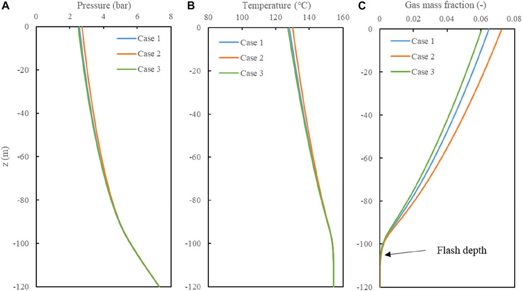
FIGURE 15. Effect of calculation parameters based on ZK304.
6.4 Application prospect of the two-phase wellbore flow model in geothermal field
The two-phase wellbore flow model constructed by this paper has great application prospect. Firstly, it can be used to estimate the production performance parameters (such as wellhead temperature, pressure and dryness) which is very useful for new geothermal wells drilling. It can be coupled with reservoir simulators to evaluate the change in wellhead temperature, pressure and dryness as the geothermal development. Secondly, it is basis for calcite scaling evaluation which is very important for the injection of chemical anti-scaling inhibitor and descaling. The wellbore calcite scaling includes four important coupled process: two-phase flow with phase transition, water-gas-mineral reaction, solute transport and wall adhesion (Figure 16). Based on the these coupled models, the profile of the thickness of calcite scaling can be obtained, which is the future work. In the evaluation of calcite scaling, the two-phase wellbore flow would provide key parameters such as pressure, temperature, saturation and velocity for the following calculation of reactive transport. Thirdly, combination of the wellbore pressure-temperature measurement and two-phase model calculation, the CO2 content in the reservoir can be inversely identified. Fourthly, it can be used to help design the separator at the wellhead and fluid (including gas and liquid phase) transportation pipeline.
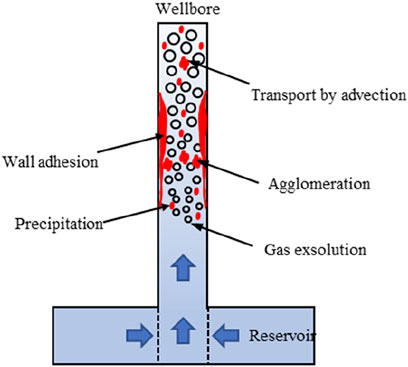
FIGURE 16. Conceptual map for calcite scaling in wellbores.
7 Summary and conclusion
The Yangbajing geothermal field in Tibet is one of the typical high-temperature geothermal fields and is the first to be used for high-temperature power generation in China. During the development, numerous problems were encountered, such as resource depletion and wellbore scaling. In order to deeply understand these problems, this paper analyzes the two-phase flow in the typical production wells and the findings can be summarized as follows.
(1) Temperature and pressure measurements during the self-discharge testing revealed that the temperature in the shallow geothermal reservoir is about 150°C and the pressure is around 7–8 bar at a depth of a 100 m. During the self-discharge testing, the wellhead pressure for all three wells was measured to be 2–3 bar. The temperature was 118°C–135°C at a depth of 10 m.
(2) A steady-state two-phase flow model for production wells is constructed based on the mass, energy and momentum equations. The difference between gas and liquid velocities (drift flux model) has a decisive impact on the temperature and pressure profiles. For a small diameter wellbore, the Shi et al. (2005) model has a better fitting result. For a large diameter wellbore, the Hibiki and Ishii. (2003) model shows a better performance.
(3) According the optimal simulated results, the flash depths for ZK324, ZK303 and ZK304 without considering CO2 are 44.9, 112.5 and 97.7 m, respectively. If the CO2 content in fluid at the bottom of casing pipe is half of the saturation content, the flash depths would increase to 58.1, 119.5 and 107.2 m, respectively. The wellhead temperatures would be 134, 125°C and 128 °C and the wellhead pressures would be 3.1, 2.3 and 2.6 bar, respectively. The wellhead gas-phase mass fractions for the three wells are between 3% and 8%.
(4) Both wellhead temperature and pressure increase with the production rate, but the gas mass fraction decreases. When the production rate reduces to half the value of the testing rate, the wellhead temperature and pressure reduce by a range of 3°C–6°C and 0.25–0.45 bar, respectively.
The model in this study only considers a steady state and a transient two-phase flow model still needs to be developed in the future. Additionally, the wellbore model should be coupled with a reservoir model to evaluate the effects of reservoir pressure depletion on the production. Furthermore, the lack of CO2 mass fraction measurements in the fluid samples at the downhole needs still needs addressing, as the CO2 mass fraction is a key parameter for accurately evaluating the flash depth.
Data availability statement
The original contributions presented in the study are included in the article/Supplementary Material, further inquiries can be directed to the corresponding author.
Author contributions
HL: Writing-original draft, Software, Formal analysis; YX: Funding acquisition, Data curation; JL: Investigation, Formal analysis; XH: Project administration, Investigation.
Funding
This work was jointly supported by the CNNC’s centralized R & D project “Research on Key Technologies of geothermal exploration, development and utilization” and the Science and Technology Innovation Talents Project of Sichuan Province, China (No. 2022jdrc0027).
Conflict of interest
YX was employed by CNNP Kunhua Energy Development Co. Ltd
The remaining authors declare that the research was conducted in the absence of any commercial or financial relationships that could be construed as a potential conflict of interest.
Publisher’s note
All claims expressed in this article are solely those of the authors and do not necessarily represent those of their affiliated organizations, or those of the publisher, the editors and the reviewers. Any product that may be evaluated in this article, or claim that may be made by its manufacturer, is not guaranteed or endorsed by the publisher.
References
Barelli, A., Corsi, R., Pizzo, D., and Scali, C. (1982). A two-phase flow model for geothermal wells in the presence of non-condensable gas. Geothermics 11 (3), 175–191. doi:10.1016/0375-6505(82)90026-8
Battistelli, A., Calore, C., and Pruess, K. (1997). The simulator TOUGH2/EWASG for modelling geothermal reservoirs with brines and non-condensible gas. Geothermics 26 (4), 437–464. doi:10.1016/s0375-6505(97)00007-2
Bjornsson, G., Arason, P., and Bodvarsson, G. S. (1993). The wellbore simulation HOLA version 3.1. Berkeley: Earth Science Division, Lawrence Berkeley National Laboratory, University of California.
Canbaz, C. H., Ekren, O., and Aksoy, N. (2022). Review of wellbore flow modeling in CO2-bearing geothermal reservoirs. Geothermics 98, 102284. doi:10.1016/j.geothermics.2021.102284
Chen, L., Booker, J. R., Jones, A. G., Wu, N., Unsworth, M. J., Wei, W., et al. (1996). Electrically conductive crust in Southern Tibet from INDEPTH magnetotelluric surveying. Science 274 (5293), 1694–1696. doi:10.1126/science.274.5293.1694
China Geological Survey of Natural Resources Ministry (2018). China geothermal energy development report. Beijing: China Petrochemical Press.
Deendarlianto, K., and Itoi, R. (2021). Numerical study of the effects of CO2 gas in geothermal water on the fluid flow characteristics in production wells. Eng. Appl. Comput. Fluid Mech. 15, 111–129. doi:10.1080/19942060.2020.1862709
Duo, J. (2003). The basic characteristics of the Yangbajing geothermal field-A typical high temperature geothermal system. Eng. Sci. 5 (1), 42–47. (in Chinese, with English summary).
Gunn, C., and Freeston, D. (1991). “An integrated steady-state wellbore simulation and analysis package,” in Proceedings of the 13th New Zealand geothermal workshop (Auckland NZ: University of Aukland), 161–166.
Guo, Q. (2012). Hydrogeochemistry of high-temperature geothermal systems in China: A review. Appl. Geochem. 27, 1887–1898. doi:10.1016/j.apgeochem.2012.07.006
Guo, Q., Wang, Y., and Liu, W. (2007). Major hydrogeochemical processes in the two reservoirs of the Yangbajing geothermal field, Tibet, China. J. Volcanol. Geotherm. Res. 166, 255–268. doi:10.1016/j.jvolgeores.2007.08.004
Guo, Q., Wang, Y., and LiuO, W. H. (2010). O, H, and Sr isotope evidences of mixing processes in two geothermal fluid reservoirs at Yangbajing, Tibet, China. Environ. Earth Sci. 59, 1589–1597. doi:10.1007/s12665-009-0145-y
Guo, Q., and Wang, Y. (2009). Trace element hydrochemistry indicating water contamination in and around the Yangbajing geothermal field, Tibet, Chinal. Bull. Environ. Contam. Toxicol. 83, 608–613. doi:10.1007/s00128-009-9812-7
Hasan, A. R., and Kabir, C. S. (2010). Modeling two-phase fluid and heat flows in geothermal wells. J. Petroleum Sci. Eng. 71, 77–86. doi:10.1016/j.petrol.2010.01.008
Hibiki, T., and Ishii, M. (2003). One-dimensional drift-flux model for two-phase flow in a large diameter pipe. Int. J. Heat Mass Transf. 46, 1773–1790. doi:10.1016/s0017-9310(02)00473-8
Huttrer, G. W. (2021). “Geothermal power generation in the world 2015-2020 update report,” in World geothermal congress 2021, 2021 (Iceland: Reykjavik).
Jiang, J. (2012). China’s energy policy 2012. Beijing, China: Information Office of the State Council.
Lei, H. W., Bai, B., and Cui, Y. X. (2022). Quantitative assessment of calcite scaling of a high temperature geothermal production well: Two-phase flow——application to the yangbajing geothermal fields, Tibet. In Press. Wuhan: China University of Geosciences, Wuhan. Avaliable At: https://kns.cnki.net/kcms/detail/42.1874.P.20220527.1158.008.html.
Lei, H. W., Li, J., Li, X. C., and Jiang, Z. (2016). EOS7Cm: An improved TOUGH2 module for simulating non-isothermal multiphase and multicomponent flow in CO2-H2S-CH4 brine systems with high pressure, temperature and salinity. Comput. Geosciences 94, 150–161. doi:10.1016/j.cageo.2016.06.011
Li, Y. M., Pang, Z. H., and Galeczka, I. M. (2020). Quantitative assessment of calcite scaling of a high temperature geothermal well in the Kangding geothermal field of Eastern Himalayan Syntax. Geothermics 87, 101844. doi:10.1016/j.geothermics.2020.101844
Li, Y. S., Zhang, J. F., Li, Z. H., Luo, Y., Jiang, W., and Tian, Y. (2015). Measurement of subsidence in the Yangbajing geothermal fields, Tibet, from TerraSAR-X InSAR time series analysis. Int. J. Digital Earth 9, 697–709. doi:10.1080/17538947.2015.1116624
Lund, J. W., Huttrer, G. W., and Toth, A. N. (2022). Characteristics and trends in geothermal development and use, 1995 to 2020. Geothermics 105, 102522. doi:10.1016/j.geothermics.2022.102522
Lund, J. W., and Toth, A. N. (2021). Direct utilization of geothermal energy 2020 worldwide review. Geothermics 90, 101915. doi:10.1016/j.geothermics.2020.101915
Lund, J. W., Bjelm, L., Bloomquist, G., and Mortensen, A. K. (2008). Characteristics, development and utilization of geothermal resources – a Nordic perspective. Episodes 31(1), 140–147. doi:10.18814/epiiugs/2008/v31i1/019
Pan, L. H., and Oldenburg, C. M. (2014). T2Well-An integrated wellbore-reservoir simulator. Comput. &Geosciences 65, 46–55. doi:10.1016/j.cageo.2013.06.005
Rouhani, S. Z., and Axelsson, E. (1970). Calculation of void volume fraction in the sub cooled and quality boiling regions. Int. J. Heat Mass Transf. 13, 383–393. doi:10.1016/0017-9310(70)90114-6
Shi, H., Holmes, J. A., Durlofsky, L. J., Aziz, K., Diaz, L. R., Alkaya, B., et al. (2005). Drift-flux modeling of two-phase flow in wellbores. SPE 10, 24–33. doi:10.2118/84228-pa
Tonkin, R. A., O’Sullivan, M. J., and O’Sullivan, J. P. (2021). A review of mathematical models for geothermal wellbore simulation. Geothermics 97, 102255. doi:10.1016/j.geothermics.2021.102255
Vasini, E. M., Battistelli, A., Berry, P., Bondua, S., Bortolotti, V., Cormio, C., et al. (2018). Interpretation of production tests in geothermal wells with T2Well-EWASG. Geothermics 73, 158–167. doi:10.1016/j.geothermics.2017.06.005
Woldesemayat, M. A., and Ghajar, A. J. (2007). Comparison of void fraction correlations for different flow patterns in horizontal and upward inclined pipes. Int. J. Multiph. Flow 33, 347–370. doi:10.1016/j.ijmultiphaseflow.2006.09.004
Xu, D., Jing, T., and Tan, J. (2018). Analysis of production wells monitoring and its impacts in Yangbajing geothermal field. Sino-Global Energy 23, 23–28. (in Chinese, with English summary).
Zhang, L., Chen, S., and Zhang, C. (2019). Geothermal power generation in China: Status and prospects. Energy Sci. Eng. 7, 1428–1450. doi:10.1002/ese3.365
Zhang, Y., Pan, L., Pruess, K., and Finsterle, S. (2011). A time-convolution approach for modeling heat exchange between a wellbore and surrounding formation. Geothermics 40 (4), 261–266. doi:10.1016/j.geothermics.2011.08.003
Zhao, P., Duo, J., Liang, T., Jin, J., and Zhang, H. (1998). Characteristics of gas geochemistry in Yangbajing geothermal field, Tibet. Chin. Sci. Bull. 43 (21), 1770–1777. doi:10.1007/bf02883369
Zhou, D. J. (2003). Operation, problems and countermeasures of yangbajing geothermal power station in Tibet. Electr. Power Constr. 24 (10), 1–9. (in Chinese, with English summary).
Zhu, J., Hu, K., Lu, X., Huang, X., Liu, K., and Wu, X. (2015). A review of geothermal energy resources, development, and applications in China: Current status and prospects. Energy 93, 466–483. doi:10.1016/j.energy.2015.08.098
Keywords: geothermal, two-phase flow, carbon dioxide, numerical simulation, Yangbajing geothermal field
Citation: Lei H, Xie Y, Li J and Hou X (2023) Modeling of two-phase flow of high temperature geothermal production wells in the Yangbajing geothermal field, Tibet. Front. Earth Sci. 11:1019328. doi: 10.3389/feart.2023.1019328
Received: 15 August 2022; Accepted: 13 February 2023;
Published: 01 March 2023.
Edited by:
Antoni Camprubí, National Autonomous University of Mexico, MexicoReviewed by:
Yingchun Wang, Chengdu University of Technology, ChinaSukru Merey, Batman University, Türkiye
Copyright © 2023 Lei, Xie, Li and Hou. This is an open-access article distributed under the terms of the Creative Commons Attribution License (CC BY). The use, distribution or reproduction in other forums is permitted, provided the original author(s) and the copyright owner(s) are credited and that the original publication in this journal is cited, in accordance with accepted academic practice. No use, distribution or reproduction is permitted which does not comply with these terms.
*Correspondence: Hongwu Lei, aG9uZ3d1bGVpMjAwOEBhbGl5dW4uY29t