 Lukas Maderer1
 Edouard Kaminski
 João A. B. Coelho
 Véronique Van Elewyck
94% of researchers rate our articles as excellent or good
Learn more about the work of our research integrity team to safeguard the quality of each article we publish.
Find out more
ORIGINAL RESEARCH article
Front. Earth Sci., 14 March 2023
Sec. Solid Earth Geophysics
Volume 11 - 2023 | https://doi.org/10.3389/feart.2023.1008396
This article is part of the Research TopicCollaborative Exploration of Earth’s InteriorView all 8 articles
In the last 70 years, geophysics has established that the Earth’s outer core is an FeNi alloy containing a few percent of light elements, whose nature and amount remain controversial. Besides the classical combinations of silicon and oxygen, hydrogen has been advocated as the only light element that could account alone for both the core density and velocity profiles. Here we show how this question can be addressed from an independent viewpoint, by exploiting the tomographic information provided by atmospheric neutrinos, weakly-interacting particles produced in the atmosphere and constantly traversing the Earth. We evaluate the potential of the upcoming generation of atmospheric neutrino detectors for such a measurement, showing that they could efficiently detect the presence of 1 wt% hydrogen in the Earth’s core in 50 years of concomitant data taking. We then identify the main requirements for a next-generation detector to perform this measurement in a few years timescale, with the further capability to efficiently discriminate between FeNiH and FeNiSixOy core composition models in less than 15 years.
The determination of the composition of the Earth core is a long-standing debate in Earth sciences [e.g., Birch (1961); Poirier (1994); Hirose et al. (2013); McDonough (2003)]. Seismology combined with experimental petrology shows that the inclusion of a few percent of light elements is required to account for the density and seismic velocity profiles in the core, e.g., PREM (Dziewonski and Anderson, 1981). Si, O, S, C, and H (and some of their combinations) are the most popular elements that have been considered so far. The precise nature of the light elements in the core however remains elusive, and various combinations of, e.g., Si and O (Kaminski and Javoy, 2013; Badro et al., 2015), can equally fit PREM. Hydrogen, the most abundant element in the proto-solar nebula, has received a renewed interest in the past years based on high-pressure/high-temperature experiments that confirmed the possibility to put a significant amount of H in the core (Sakamaki et al., 2009; Tagawa et al., 2021). Furthermore, it is the only candidate that could account for both the density and velocity profiles in the core without the need for any additional light element (Umemoto and Hirose, 2015; Sakamaki et al., 2016; Yuan and Steinle-Neumann, 2020).
The presence of light elements in the core bears important consequences for the dynamics and formation of the Earth and of its magnetic field [Hirose et al. (2013)]. The latter rises from convection in the liquid outer core, a key question being the mechanism allowing the convective process to be efficient enough to sustain a geodynamo. Because light elements partition in the liquid phase during crystallization of the inner core, they increase the intensity of convection in the outer core, that becomes then a thermo-chemical process. This in turn improves the efficiency of cooling of the core, thereby decreasing its temperature and causing further delay in the crystallization process. Determining the precise composition of the core is therefore of prime importance to better understand the conditions of its segregation, and more generally to help discriminate different scenarios of Earth formation. For example, the relative amount of oxygen to silicon depends both on pressure and temperature conditions during iron formation, and on the nature of the material that formed the Earth. An oxygen-rich core would be expected if carbonaceous chondrites were the building blocks of the Earth, whereas a silicon-rich core would rather correspond to Enstatite chondrites.
If hydrogen is the dominant light element in the core, a very different scenario would be at play as the Mg/Si ratio of the mantle—which is non-chondritic—will be very close to that of the bulk Earth. A hydrogen-rich core would furthermore completely change the H2O bulk content of the Earth, increasing it up to 75 equivalent of the ocean content (Tagawa et al., 2021). Up to now however there has been no method available to directly constrain the amount of H in the core. The aim of the present study is to show how the development of high-performance detectors of atmospheric neutrinos opens a new path to independently constrain the composition of the core and test the FeNiH hypothesis in particular.
Neutrinos are neutral elementary particles that exist in three flavors: electron (e), muon (μ) and tau (τ). Because they feel only the weak interaction, they can traverse and emerge from very dense media, including the Earth itself, without losing energy during their propagation. The interactions of cosmic rays with the atmosphere generate an abundant and ubiquitous flux of energetic neutrinos, which undergo flavor oscillations while crossing the Earth (Fukuda et al., 1998). The probability of their flavor transition depends on the neutrino energy and path length, but also on the density of electrons ne in the traversed medium (Wolfenstein, 1978; Mikheyev and Smirnov, 1985). Because of its dependence in ne, this effect is key in accessing chemical properties of the traversed medium through neutrino oscillation physics. Assuming an Earth’s radial structure and composition, ne as a function of r, the radial distance from the center of the Earth, is given by
where
where Zi, Ai and wi are respectively the local atomic number, standard atomic weight and weight fraction of element i of the material. Chemical elements with different Z/A will therefore generate distinct signals in the neutrino oscillation pattern for a given mass density. The signature of these oscillations in the atmospheric neutrino signal observed at a detector can thus reveal the nature of the matter they interacted with.
While this method of Earth tomography has been conceptually explored in different contexts since the 1980s [see, e.g., Ermilova et al. (1986); Nicolaidis (1988); Nicolaidis et al. (1991); Ohlsson and Winter (2001); Ohlsson and Winter (2002); Lindner et al. (2003); Winter (2006) and references therein], only now does the upcoming generation of atmospheric neutrino detectors provide a concrete opportunity to evaluate its capability of probing the density and/or composition of the deep Earth. Oscillation tomography with atmospheric neutrinos has been recently discussed by several authors (Rott et al., 2015; Winter 2016; Bourret et al., 2018; Bourret and Van Elewyck, 2019; D’Olivo et al., 2020; Kumar and Agarwalla, 2021; Denton and Pestes, 2021; Kelly et al., 2022; Capozzi and Petcov, 2022; D’Olivo Saez et al., 2022), with a variety of approaches in the treatment of the neutrino signal and in the targeted geophysical observables. In this study, we propose to re-examine the relevance and potential of this method for the characterization of the Earth’s core composition, with a specific focus on its capacity to identify and quantify the presence of Hydrogen in the core. This topical question for the geoscience community indeed appears as a promising area of application of neutrino oscillaton tomography thanks to the very large Z/A of H compared to Fe and other light elements.
Section 2 describes the theoretical background, the methods and inputs used for the computations that support the present study. Our main results on neutrino oscillation tomography of the Earth’s outer core are presented in Section 3. We start in Section 3.1 by quantifying the expected theoretical reach of the method under the hypothesis of perfect detector capabilities, showing how different assumptions for the outer core composition will indeed modify the number of neutrinos of different flavours interacting at a detector site. In Section 3.2 we move to investigating the realistic performances of the two main families of atmospheric neutrino detectors presently under construction, and discuss their ability to detect the presence of 1wt% Hydrogen in the outer core. Finally, we illustrate in Section 3.3 the evolution required for the next-generation of detectors to be able to discriminate FeNiH vs. FeNiSixOy models of the Earth’s core. The context and implications of our findings are further discussed in Section 4.
Neutrino flavor oscillations are a quantum-mechanical phenomenon that arises because the neutrino flavor eigenstates νe, νμ, ντ—which take part in weak interactions and are therefore the observable states—are not identical to the neutrino mass eigenstates ν1, ν2, ν3—which describe their propagation in vacuum. The flavor eigenstates are a quantum superposition of the mass eigenstates, whose relative phases change along the neutrino propagation path. This evolving mix of states leads to an oscillatory pattern of the detection probability of a given neutrino flavor, which depends on the neutrino energy and traveled distance.
Neutrino oscillation probabilities are calculated by solving the Schrödinger equation i∂t|ν(t)⟩ = H|ν(t)⟩. The neutrino propagation Hamiltonian H is approximated as the sum of two terms:
The first term represents intrinsic energy levels of the system in vacuum. Because neutrinos are generally observed in an ultra-relativistic context, the energy difference between mass states is approximately proportional to their difference in mass-squared
The second term in Eq. 3 arises from coherent interactions of neutrinos with electrons in the medium in which they propagate (Wolfenstein, 1978; Mikheyev and Smirnov, 1985). The effective potential
The solution of the Schrödinger equation for such a system in matter of constant density amounts to computing the eigensystem of the full Hamiltonian. While in vacuum the eigenvalues and eigenvectors are given by
For example, the effective mixing angle
with a mapping parameter
At the energy and distance scales relevant to atmospheric neutrino oscillations, the probability of observing a transition between νe and νμ flavors is proportional to sin22θ13, which is small in vacuum, as observed in oscillation measurements of reactor antineutrinos (Abe et al., 2012; Ahn et al., 2012; An et al., 2012) that are insensitive to the matter potential. However, the νe ↔ νμ transition probability may become large or even maximal when ξ2 → sin22θ13, which translates into a resonance condition for the neutrino energy:
Neutrinos traversing the Earth will experience resonant oscillations in the outer core for energies ∼3 GeV, and in the mantle for ∼7 GeV, with the exact resonant energy depending on the electron density of the material.
An almost isotropic neutrino flux is constantly produced by the interaction of cosmic rays with air molecules, mainly coming from the decays of charged mesons (π±’s and K±’s) and muons. At energies above 100 Megaelectron Volts (MeV) approximately, these atmospheric neutrinos become the dominant neutrino flux observed on Earth. It occurs noting here that such energies are well above the ones (∼ few MeVs) typically attained by geoneutrinos, the electron (anti-)neutrinos produced in nuclear decays of radioactive elements like 238U, 232Th and 40K, which are responsible for the Earth’s radiogenic heat flux (Smirnov, 2019). While geoneutrinos have their own intrinsic interest for inferring information about the Earth’s composition, they can be safely ignored in the present study which focuses on neutrinos with energies of 1 Gigaelectron Volt (103 MeV) and above.
Atmospheric neutrino flux calculations rely on 3D Monte-Carlo simulations of air shower development, starting with a primary cosmic ray flux based on measurements, and including solar modulation, geomagnetic field effects and seasonal variations of the atmosphere density. For the present study, we use as input the flux produced by Honda et al. (2015) for the Gran Sasso site (without mountain over the detector), averaged over all azimuth angles and over seasonal variations, and assuming minimum solar activity. The flux is dominated by muon- and electron-(anti)neutrino components, with an approximate ratio of 2:1 between νμ and νe flavors, and we have neglected the small contribution of
For a given zenith angle of incidence θz, as defined in Figure 1A, the neutrino trajectory across the Earth is modelled along the corresponding baseline through a sequence of steps of constant electron density which are inferred from a radial model of the Earth with 42 concentric shells of constant ne, where mass density values are fixed and follow PREM. These shells are grouped into three petrological layers (inner core, outer core, and mantle+crust), whose composition, hence Z/A factor, is assumed to be uniform and provided in Table 1). In each shell, the electron density is determined from the mass density and Z/A according to Eq. 2. The probabilities of neutrino flavor transitions along their path through the Earth are computed using the OscProb 2 package. The values of the parameters that enter the oscillation probability computation are taken from the global fit of neutrino data performed with the NuFIT analysis Version 5.0 (Esteban et al., 2020). We have assumed normal ordering of the neutrino mass states, i.e., m3 > m1, which is currently favoured by NuFIT and other global fits of neutrino data (Capozzi et al., 2021; de Salas et al., 2021).

FIGURE 1. Oscillations of Earth-crossing neutrinos. (A): A detector located at the surface will receive atmospheric neutrinos having traversed the Earth along different paths, as measured by their zenith angle θz with respect to the vertical at the detector location. As these neutrinos cross the Earth, the amplitude of their oscillations at different depths will be affected by the local density of electrons. A modification in the electron density of the outer core would then affect the flavor mix of neutrinos that cross it. (B). To illustrate this effect, the number of interactions expected for atmospheric muon neutrinos and antineutrinos
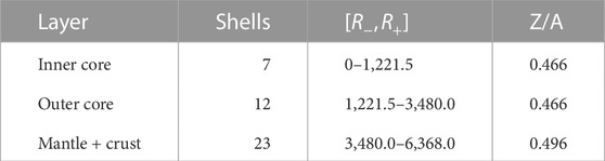
TABLE 1. Compositional layers in the benchmark Earth model used in the analysis when assuming a pure FeNi outer core. The columns indicate the number of constant density shells (each of them taking its value from PREM), the exact innermost and outermost radius (in km) and the assumed Z/A value.
Neutrinos with energies in the range
The rate of neutrinos interacting in a given volume of target matter is then computed, for each interaction channel α (NC/CC; e, μ, τ;
where we have made explicit the dependence on the neutrino energy E and on the incoming zenith angle θz, as defined in Figure 1A, under the assumption of a spherically symmetric mass density profile of the Earth. The angle θz is directly related to the path length L through the Earth: L ≈ − 2R⊕ cos θz with R⊕ the radius of the Earth.
Neutrinos are observed only indirectly, through the signal deposited in the detector by the byproducts of their interaction. The ability to detect, reconstruct an identify the different types of neutrino events in the energy range of interest for Earth tomography is essentially driven by the detector size, technology and density of sensors. We consider here two main experimental approaches that are currently pursued for the upcoming generation of detectors targeting neutrinos with energies at the GeV scale, and that rely on different detection materials and observation strategies:
• Liquid Argon (LAr) detectors are a type of Time Projection Chamber (TPC) (Rubbia, 1977) that detects the electrons released upon ionization of Argon atoms along the paths of the secondary charged particles emerging from the neutrino interaction.
• Water-Cherenkov (wC) detectors instrument large volumes of water (or ice) with arrays of photosensors that detect the Cherenkov light induced by the secondary charged particles traveling faster than light in water (Tamm and Frank, 1937; Čerenkov, 1937).
LAr TPCs are able to reconstruct highly detailed 3D images of the neutrino event, providing excellent flavor identification capabilities, even at low (sub-GeV) energies, and energy and angular resolutions typically superior to water-Cherenkov detectors. The size of these detectors is however limited by their much higher cost. The first large-scale LArTPC detector was the ICARUS T600 detector (Rubbia et al., 2011), with an active mass of 476 tons. A new generation of LArTPCs is being developed for the DUNE experiment (Abi et al., 2020c), that will include four detectors of 10 kton active mass each.
The performance of water-Cherenkov detectors, on the other hand, is typically a trade-off between the target volume for neutrino interactions and the density of photosensors that sample the Cherenkov signal emitted by charged byproducts of the neutrino interaction. The Hyper-Kamiokande experiment (Abe et al., 2018) will consist in two
To simulate the detector response, we use a set of parametrized analytical functions modeling the main performance features relevant for the detection, reconstruction and classification of neutrino events:
• The effective mass Meff(E) is the product of the instrumented target mass M of the detector and its detection efficiency, i.e., the probability for a neutrino interaction to be successfully detected as an event. Meff typically increases with the neutrino energy, until reaching a plateau that saturates the fiducial mass of the detector. We have conservatively neglected here a potential increase in Meff for νμ CC events at high energies, corresponding to through-going muons created in neutrino interactions outside of the detector target volume. The threshold for detection is mainly driven by the density (and intrinsic efficiency) of sensors. We approximate Meff(E) by a sigmoid function of log(E) with two adjustable parameters Eth and Epl, which correspond to energies where the detection efficiency reaches 5% and 95% respectively.
• The energy resolution parameterizes the relative error on the reconstructed neutrino energy in the form of a Gaussian probability distribution function (p.d.f.) with energy-dependent width:
• The angular resolution parameterizes the error on the measured zenith angle in the form of a von Mises-Fisher p.d.f. on a sphere marginalized with respect to azimuth. For wC detectors we take into account the dependence of σθ on the energy as
• The classification efficiency ɛclass(E) describes the probability for a neutrino event of energy E to be correctly classified into one of the topological channels observable by the detector. We model it with a sigmoid as a function of log(E) with adjustable threshold
Events are classified according to their topological features, which depend on the signature of each interaction channel (NC/CC;
In this study we assume that all detectors under consideration have the basic capability to classify events into two main observational classes: track-like events, which are mostly associated to νμ charged-current interactions producing a long muon track, and cascade-like events, when there is no such single muon or the muon energy is too small for it to be distinguished among the many other secondary particles created in the event. The cascade channel therefore comprises mainly νe CC and (subdominantly) ντ CC interactions, plus a small contribution from νμ CC interactions without an observable muon, and all NC interactions.
For NC interactions, a fraction of the energy of the event is carried away by an invisible outgoing neutrino, resulting in a lower reconstructed energy and degraded angular resolution. Because NC-induced events are blind to neutrino flavor, they only decrease the experiment sensitivity. Fine-grained detectors like DUNE and Hyper-Kamiokande have some capability to separate and reject the NC-induced events from the νe CC events, thereby increasing the flavor purity of the cascade channel. To account for a possible related improvement in the detector sensitivity, we have considered here both the baseline case that includes the NC-induced events in the cascade sample, and the optimistic case where the NC-induced contributions are completely removed from the sample. We have also used throughout our study the neutrino-nucleon cross-sections weighted for water molecules obtained with the GENIE Monte Carlo neutrino generator (Andreopoulos et al., 2010), neglecting the small difference in cross-section for interactions on Argon nuclei in the case of the DUNE detector.
In order to obtain the expected signal in a realistic experiment, the rate of interacting neutrinos as obtained from Eq. 7 must be weighted with the appropriate detection efficiency at each incoming neutrino energy. In the following we use the subscript “true” for the quantities (energy and zenith angle) that refer to the incoming neutrino properties, and “reco” for their reconstructed values as provided by a given detector. The observed event rate is computed by a discretized convolution of the interacting rate at energy Etrue and incident at zenith angle θtrue over the E-cos θ plane according to the energy and zenith resolution p.d.f.s. The reconstructed events for each interaction channel are distributed into the two observational channels (tracks and cascades) according to the classification efficiency function ɛclass(E). Every bin in the final (Ereco, θreco) event oscillogram therefore (i) contains a certain fraction of misreconstructed events coming from other (Etrue, θtrue) bins; and (ii) misses some events that end up misreconstructed into different (Ereco, θreco) bins.
The final event rate expected in a given channel, in a given bin of reconstructed energy and zenith angle, is thus obtained as follows for the track channel:
where PDFangle and PDFenergy represent the probability distribution functions of the angular and energy resolutions as defined above. A similar expression can be straightforwardly derived for the event rate in the cascade channel.
Independently of any classical measurement error, the intrinsically probabilistic nature of neutrino interactions as a quantum process induces a statistical uncertainty on the number of events observed in each bin of (Ereco, θreco). Our statistical analysis is based on the standard Asimov dataset approach, in which all observed quantities are set equal to their expected values. The probability to detect N neutrino events of a given topology, e.g., tracks, in a predetermined interval of reconstructed energy and zenith angle is distributed according to a Poisson law, parametrized by the expected number of events
Once these fluctuations are taken into account, we compute the log-likelihood ratio λLLR of the resulting event histograms, which yields a measure of the significance to reject model B (the “test hypothesis”) if model A (the “null hypothesis”) is true. According to Wilk’s theorem, for large enough statistics, the Poisson-distributed events converge towards a normal distribution, so that −2λLLR can be approximated by:
The total Δχ2 (integrated over all bins of energy and zenith angle) is related to the significance
Based on the simulation chain described in Section 2, our first step is to evaluate the intrinsic sensitivity of the method by conducting detailed computations of the propagation of neutrinos through the Earth and comparing the expected rate of interacting neutrino events in a perfect detector under different assumptions for the outer core composition.
From Eq. 7, one can generate the two-dimensional (2D) distributions of expected number of neutrino interactions of a given flavor as a function of (E, θz), or oscillograms, for any specific exposure of a perfect detector that would observe atmospheric neutrinos from all directions. Because of the dependence of neutrino oscillation on ne along the neutrino path, changes in the outer core composition (i.e., different Z/A) induce variations in the expected signal, depending on the neutrino energy and exact trajectory (or equivalently, θz), that get imprinted in the oscillograms.
We have quantified this effect by computing the relative difference (ΔN/N) in expected number of neutrino events between oscillograms generated with different models of outer core composition. We considered five different models (see Table 2), ranging from a pure FeNi alloy to a Hydrogen-rich (FeNiH) one, with two intermediate models chosen from the FeNiSixOy family. As mentioned in the introduction, silicon and oxygen are not the only light elements that have been proposed in conventional models of the outer core; also sulphur and carbon could be present (Poirier, 1994), but their Z/A is too close to that of Si and O to allow for a discrimination by means of this method. Furthemore, high-pressure/high-temperature thermodynamics modelling appear to rule out Fe-Si-C compositions (Huang et al., 2022). Therefore we do not consider them further in this study.
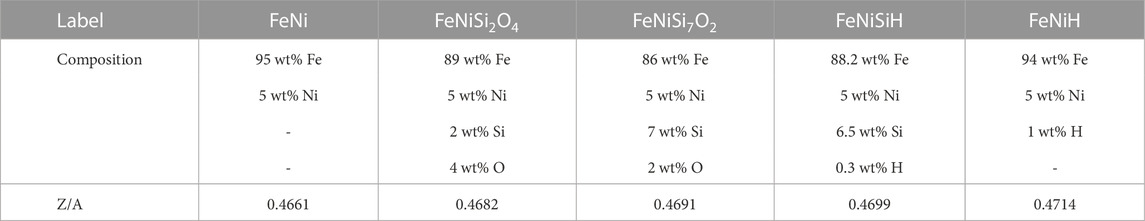
TABLE 2. Models of outer core composition considered in this study, showing the weight fraction of the different elements and corresponding average Z/A. The FeNi model is the benchmark alloy used to model the inner core composition, whereas other models introduce different combinations of light elements: FeNiSi2O4 (Badro et al., 2015), FeNiSi7O2 (Kaminski and Javoy, 2013), FeNiSiH (Tagawa et al., 2016) and FeNiH (Sakamaki et al., 2016). In all models the Ni content is set to 5 wt% and Fe is the complement to 100% once light elements have been taken into account. All elements in the table have a Z/A ranging between 0.46 and 0.50, except Hydrogen whose Z/A = 1 is responsible for pulling the average Z/A to higher values.
Figure 2 illustrates the expected impact of the composition in terms of ΔN/N for muon- and electron-neutrino interactions, as a function of the neutrino energy, for two different incoming directions. The predicted numbers of interactions for those particular configurations are shown to differ by up to 4% for electron neutrinos, and up to 17% for muon neutrinos, depending on the core composition considered. Furthermore, because the shape of the signal changes a lot depending on the zenith angle, it appears important to consider the signal in two dimensions (i.e., as a function of E and θz). This is further illustrated in Figure 3 showing the full 2D distributions of ΔN/N for muon- and electron-neutrino interactions, for a specific comparison between FeNiH and FeNi core compositions. Such results confirm that a detailed study of the neutrino event rate in the energy range 1–10 GeV has the potential to constrain the Earth’s outer core composition.
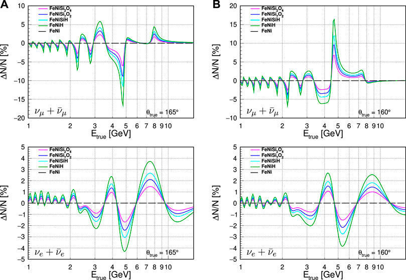
FIGURE 2. Predicted relative difference ΔN/N in the number of neutrino interactions as a function of the incoming (or “true”) neutrino energy, for the different outer core compositions described in Table 2, taking FeNi as a reference. Upper panels are for
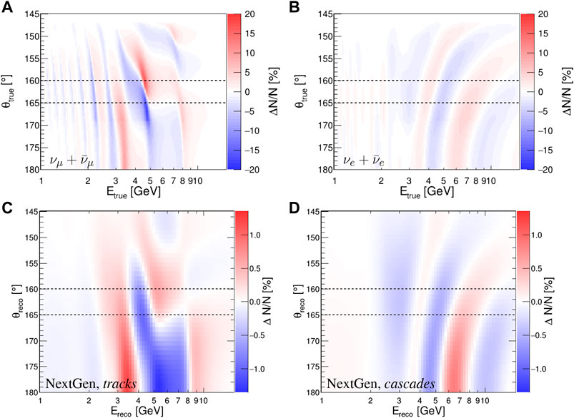
FIGURE 3. Upper panels: expected relative difference ΔN/N in the number of neutrino interactions, as a function of the incoming (or “true”) neutrino energy and zenith angle, for the composition models FeNiH vs. FeNi .(A) panel is for
The distributions shown in the upper panels of Figure 3 implicitly relate to a detector with 100% detection efficiency, perfect energy and θz resolution, and infinite statistics. In reality, the measurement accuracy will be limited by experimental effects, resulting in some blurring and attenuation of the signal, as illustrated in Figure 3 (lower panels). As discussed in Section 2.4, the detector technology and specifications (size, detection efficiency, resolution and particle identification) affect its ability to reconstruct the neutrino properties (energy, direction and flavor), and the intrinsically probabilistic nature of neutrino interactions induces a statistical uncertainty on the final observed number of events. The detector thus needs to be scalable to a sufficiently large volume for this uncertainty to be smaller than the intrinsic signal.
To investigate the influence of specific detector characteristics on their potential to constrain the core composition, we use the parametrized functions defined in Section 2.4 to model the key experimental features - namely, the effective mass, the direction and energy resolutions, and the efficiency in identifying the neutrino flavor based on the classification of events into track and cascade topologies. We consider here four benchmark parametrizations with specific inputs chosen as educated guesses for different detectors representative of the upcoming generation of GeV neutrino detectors: Hyper-Kamiokande, ORCA, and DUNE. The detail of the parameters used for each detector is provided in Table 3.
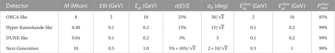
TABLE 3. Inputs for the response functions of the detectors considered in this study (as discussed in Section 3.2): total target mass; threshold and plateau energy for the detection efficiency curve; energy and zenith resolutions; threshold and plateau energy for the classification efficiency curve; maximal classification probability achievable.
The DUNE-like model (Abi et al., 2020a; 2020c; Kelly et al., 2022) accounts for the superior resolution and reconstruction capabilities of the Liquid Argon detection technique, at the cost of a much smaller instrumented volume. At the other extreme, the ORCA-like model (Adrian-Martinez et al., 2016; Aiello et al., 2022) reflects the higher detection threshold and degraded reconstruction performances that result from a sparsely instrumented - although larger - volume. The Hyper-Kamiokande-like model (Abe et al., 2018) is a middle-way option combining a medium-size detector with a low detection threshold and good reconstruction and identification capabilities, in line with those already achieved with its predecessor Super-Kamiokande (Suzuki, 2019). Although some of the detectors considered here may be sensitive to neutrinos below 1 GeV, we have conservatively limited our study to neutrinos with energy in the range [1,40] GeV, which encompasses most of the expected oscillation tomography signal. Some examples of the corresponding response functions are presented in Figure 4 for the energy range under consideration.
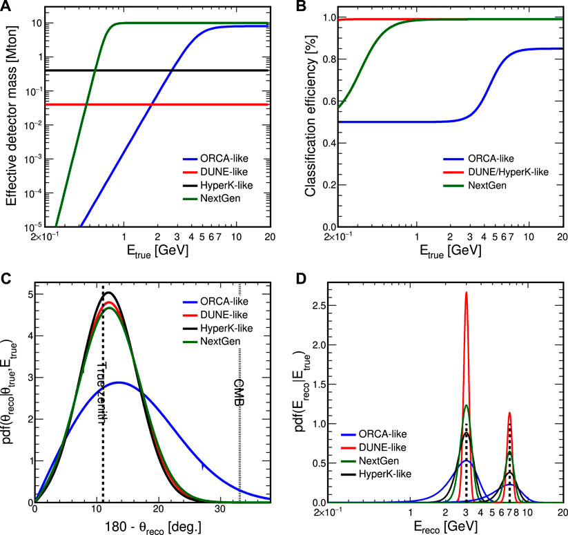
FIGURE 4. Examples of response functions used for the modelling of the neutrino detectors. (A): Effective detector mass (Meff) as a function of the neutrino true energy. (B). Classification efficiency (ρclass) as a function of the true neutrino energy. (C). Probability distribution function for the reconstructed zenith angle for a neutrino with true energy Etrue = 10 GeV and true zenith angle θtrue ≈ 169° (corresponding to a neutrino trajectory grazing the inner-outer core boundary). (D). Probability distribution function for the reconstructed energy for two specific values of the true neutrino energy (Etrue = 1 and 5 GeV).
The corresponding modelling, and the physical parameters used for each specific detector, are described in Section 2.4 and Table 3. By folding the detector response with the expected rate of neutrino interactions given by Eq. 7, and summing over all relevant interaction types, we obtain the predicted rate of observable events of a given observational class,
For a given detector, our projected experimental sensitivities are obtained from the detailed comparison of the full 2D oscillograms of expected neutrino events, generated with different assumptions for the core composition. As described in Section 2.5, a statistically meaningful way of quantifying the detector performance is to apply a χ2 hypothesis test to the 2D histograms of expected events in bins of (Ereco, θreco). Under the assumption of the validity of Wilk’s theorem, the total Δχ2 associated to a given pair of composition models, say A and B, is directly related to the significance
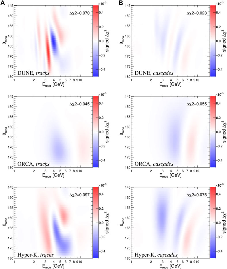
FIGURE 5. Δχ2 sensitivity for discriminating between FeNi model and FeNiH model in 20 years livetime of upcoming detectors. From top to bottom, the panels show the signed Δχ2 maps (as defined in Section 2.5) as a function of the reconstructed neutrino energy and zenith angle, for DUNE, ORCA, and Hyper-Kamiokande, for track-like events (A) column and cascade-like events (B) column as defined in Section 2.4. The color scale is the same in all plots. The number indicated in each plot corresponds to the total Δχ2 sensitivity summed (in absolute value) over all bins of the (Ereco, θreco) plane.
Figure 6 compares more directly the performances of the benchmark detectors in discriminating outer core composition models. Despite the differences in technology, size and reconstruction performances, we find that ORCA and DUNE reach a similar precision of 0.016 (at 1σ C.L.) on the absolute Z/A measurement after 20 years of data taking. These results are comparable with the ones previously published (Bourret and Van Elewyck, 2019) based on a full simulation of the ORCA detector. They confirm the capability of these detectors to measure the Z/A in the Earth’s outer core with a 1σ relative precision of 3–4 percent. Hyper-Kamiokande performs slightly better, with a relative precision of 2.5%, yielding a discrimination power of approximately 0.5σ between FeNi and FeNiH models for 25 years of measurements. A higher sensitivity can be achieved by combining the data from the three detectors into one single measurement; in that case, a 1σ C.L. discrimination power for FeNiH vs. FeNi could be reached in 50 years of concomitant data taking, as can be seen in Figure 7.
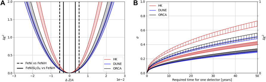
FIGURE 6. Sensitivity of the individual upcoming detectors to the outer core composition. (A) Sensitivity profile for the absolute precision in the Z/A measurement, for 20 years operation of the Hyper-Kamiokande, DUNE and ORCA detectors. The vertical lines indicate the Z/A separation between specific pairs of models of core composition. (B) Sensitivity bands as a function of the detector livetime, for discriminating specific pairs of models. In the (B) plot, the filled bands represent the discrimination power between FeNiSi2O4 and FeNiH, while the hashed bands represent FeNi vs. FeNiH. The band limits in both plots correspond to the baseline and optimistic assumptions on the detectors capability to filter out events which are insensitive to neutrino flavor (as explained in Section 2.4).
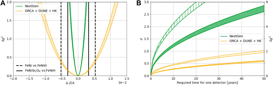
FIGURE 7. Sensitivity to the outer core composition for upcoming and next-generation detectors. (A) Δχ2 profile for the absolute precision in the Z/A measurement, for 20 years operation of a Next-Generation (NextGen) detector and for the combination of DUNE, ORCA and Hyper-Kamiokande (HK) over the same livetime. The vertical lines indicate the Z/A separation between specific pairs of models of core composition. (B) Sensitivity bands as a function of the detector livetime, for discriminating specific pairs of models. In the (B) plot, the filled bands represent the discrimination power between FeNiSi2O4 and FeNiH, while the hashed bands represent FeNi vs. FeNiH. The band limits correspond to the baseline and optimistic assumptions on the detectors capability to filter out events which are insensitive to neutrino flavor (as explained in Section 2.4).
While the previous result can be seen as a promising proof of concept of the method, achieving the next level of sensitivity requires both beating the statistical limitation by scaling up the detectors in size, and achieving excellent reconstruction performances (flavor, Ereco, θreco), in order to better resolve the patterns in the 2D (Ereco, θreco) event distributions.
Based on the results obtained for the upcoming detectors, we have investigated possible realizations of such a next-generation, or NextGen, detector, that would combine the best performances of current-generation instruments, taking as benchmarks a 1 GeV detection threshold and almost perfect (99%) discrimination between track-like and cascade-like events.
We performed a systematic scan of the discrimination potential of such detector over a large range of sizes, energy and angular resolutions, as presented in Figure 8. A separation power of at least 1σ between FeNiSi2O4 and FeNiH models can be obtained with a rather wide combination of zenith/energy resolution parameters. A good compromise is found in the region around σ(θ) = 7° angular resolution and σ(E)/E = 10% energy resolution, not far from the performances associated with Hyper-Kamiokande, but for a significantly larger, 10-Mton, detector. We provide a specific parametrization of such a NextGen detector in Table 3.
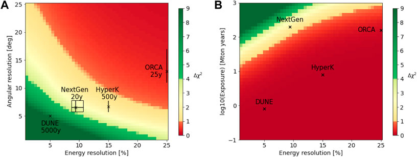
FIGURE 8. Δχ2 sensitivity for discriminating FeNiSi2O4 vs. FeNiH with a NextGen detector for various combinations of exposure, energy and angular resolutions. The (A) plot is obtained for a fixed exposure of 200 Mton yr. The color scale indicates the intervals between 1, 2, and 3 σ (68%, 95%, 99% C.L.). Superimposed on the maps are the lifetimes required to reach the 200 Mton yr exposure for DUNE, ORCA and HK detectors, as well as their specific resolution in the energy range of interest for the tomography measurement (3–7 GeV). The (B) plot is obtained by assuming a linear relationship between the energy and angular resolutions for the benchmark detectors, as suggested by the (A) plot.
This scan also illustrates how the small size and limited scalability of Liquid Argon detectors is a serious obstacle to developing this technique to achieve the required exposure levels in a reasonable running time, despite their superior energy and zenith resolution. Even an asymptotic evolution of the DUNE experiment, with perfect identification of all neutrino flavors and interaction channels, would only reach a 0.5σ discrimination power for FeNiSi2O4 vs. FeNiH after 50 years running. We conclude that better perspectives for a core composition measurement arise from the water Cherenkov approach, provided that event reconstruction and identification performances similar or better to those of Hyper-Kamiokande can be achieved in a much larger (hence likely more sparsely instrumented) detector.
The performance of the NextGen detector is illustrated in Figure 9 in terms of the signed Δχ2 maps for the discrimination between a FeNiH and a FeNiSi2O4 composition of the outer core, for the track and cascade channels, for 20 years of data taking. In this example, the total Δχ2 value is 2.71, respectively 1.68 for track and 1.03 for cascade channel.
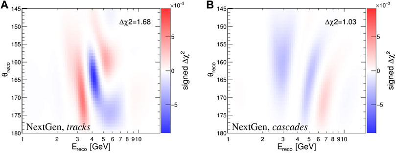
FIGURE 9. Sensitivity of the NextGen detector for discriminating between FeNiSi2O4 and FeNiH outer core compositions after 20 years data taking. The plots show the signed Δχ2 maps (as defined in Eq. 9) as a function of the reconstructed energy and zenith of the neutrinos, respectively for track-like (A) and cascade-like (B) events.
The qualitative jump in performance that could be achieved with the NextGen detector is also evident in Figure 7 where its sensitivity is compared to the one obtained from combining ORCA, DUNE and Hyper-Kamiokande data. The characteristics of the NextGen detector yield a sub-percent precision on the Z/A measurement, sufficient to distinguish between FeNiSi2O4 and FeNiH compositions at
We further illustrate such capabilities in Figure 10, where we address the separability (at the 1σ level) between pairs of realistic core composition models, as a function of the detector running time. Although a discrimination between composition models whose Z/A are closer than 0.001 (i.e., FeNiSi7O2 vs. FeNiSi2O4, or FeNiSi2O4 vs. FeNiSiH) appears out of reach, our results suggest that the NextGen detector would be able to exclude or confirm the FeNiH hypothesis against all the other realistic models considered in this study. This result can be obtained in less than 20 years if the actual outer core composition is in the family of models with an admixture of Silicium and Oxygen as only light elements.
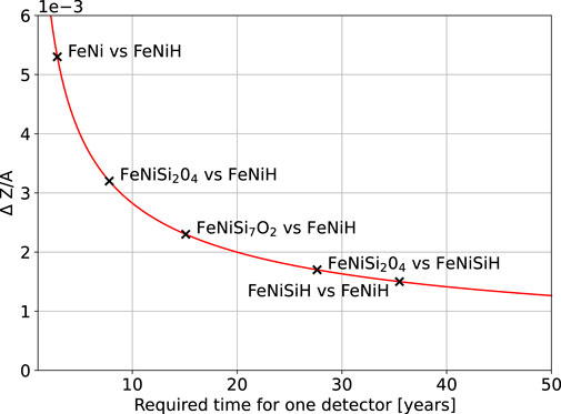
FIGURE 10. Precision of the Z/A measurement achievable at 1σ with the NextGen detector as a function of running time. The crosses indicate the separation in Z/A between pairs of models considered in this study. Not shown in the graph is the time required to distinguish FeNiSi7O2 vs. FeNiSi2O4 ( ≃ 90 years) and FeNiSi7O2 vs. FeNiSiH ( ≃ 120) years. If n identical NextGen detectors were running in parallel, the time scale would be approximately reduced by that same factor n, i.e., FeNiSi7O2 vs. FeNiSi2O4 could be distinguished in about 20 years if 4 NextGen detectors would be taking data simultaneously.
This paper presents a detailed study and comparison of the potential of upcoming atmospheric neutrino detectors to constrain the outer core composition to precision levels of relevance for geophysics. As a first step, we confirm the theoretical capability of neutrino oscillation tomography to discriminate between different realistic core composition models by computing the propagation and oscillation of atmospheric neutrinos through the Earth with well-established tools from the neutrino physics community. We note that the largest contribution to the theoretical signal is provided by atmospheric neutrinos reaching the detector in the νμ flavor, which may explain why many of the neutrino oscillation tomography studies to date have focused on this detection channel only.
The ultimate reach of this method, however, significantly depends on how the expected signal is effectively extracted in a realistic experiment. In order to address this question in a flexible way and with a view to the future, we have developed our analysis based on analytical parametrisations of the detector response functions, similar in concept to the studies by Winter (2006) and Rott et al. (2015). This approach has allowed us to investigate for the first time different classes of experiments - namely, Liquid Argon TPCs and water-Cherenkov detectors - within a unified framework, based on educated guesses on the expected performances of the different detectors. Its implementation in terms of generic detection parameters would easily allow for further refinement in the description of the detector response to different observational channels, and also for comparisons with other neutrino detection techniques that could be proposed in the future. By making our code public, we aim at providing the community with a simple, versatile simulation tool to further explore the potential of neutrino oscillation tomography.
One notable conclusion to be drawn from our study, is that the respective contribution of the different neutrino flavours reaching the detector to the total signal (in terms of discrimination power for different core composition models) can vary significantly for different choices of the parametrized response functions, hence for different detectors, even within the same experimental approach. This observation emphasizes the importance of considering the neutrino signal in all its components - here, namely, the two observational channels tracks and cascades, in order to accurately assess the expected reach of a given experiment.
We have not addressed in detail in this study the more general question of systematic uncertainties related to the production, propagation (hence, oscillation) and interaction of atmospheric neutrinos, that may affect the accuracy of the Z/A measurement. The dominant sources of error on the neutrino fluxes come from uncertainties in hadron production along the atmospheric shower development, and subdominantly from uncertainties in the primary flux (Barr et al., 2006). The oscillation probabilities of neutrinos traversing the Earth depend on the squared mass differences
The parameter having by far the largest impact on our results is the ordering of the neutrino mass eigenstates, and more specifically the (still unknown) sign of
The impact of systematic uncertainties related to the oscillation parameters and to the normalization, shape and flavour content of the atmospheric neutrino flux have been discussed more extensively in some other recent studies, both for ORCA-like (Rott et al., 2015; Winter 2016; Bourret and Van Elewyck, 2019; Capozzi and Petcov, 2022; D’Olivo Saez et al., 2022) and DUNE-like (Kelly et al., 2022) detectors, and shown to have a limited to moderate impact on tomographic measurements. In the specific case of the measurement of the core composition which is our focus here, we benefit from the fact that such systematic effects can be mitigated and controlled by exploiting the sample of neutrino events that only traverse the mantle (and not the core). Moreover, the uncertainties on both the atmospheric neutrino fluxes and the oscillation parameters (in particular on θ23, which also has a significant impact on oscillation probabilities for atmospheric neutrinos at the GeV energy scale) will significantly reduce in the course of the upcoming decade, as a result of the current neutrino experimental program. Therefore those systematics should be much better constrained by the time the detectors discussed here have accumulated sufficient statistics to efficiently investigate the Earth’s core composition.
Taking advantage of the versatility of our framework, we have further investigated the desirable detection performances for a NextGen detector that - contrarily to the upcoming generation of experiments - would be optimized for neutrino oscillation tomography. We find that such performances stem from two complementary aspects: (i) the large statistics of events provided by an experiment with 10 Mton target mass and a relatively low (∼ 1 GeV) energy threshold that fully covers the energy range where resonant oscillation effects are expected for core-crossing neutrinos; and (ii) the state-of-the-art event reconstruction and classification capabilities. Limitations to this measurement arise from the intrinsic, quantum fluctuations in the particle content of the hadronic shower that results from the fragmentation of the nucleus hit by a neutrino. These effects have been extensively discussed for ORCA-like detectors (Adrián-Martínez et al., 2017) and shown to limit the performances as long as individual particles in the neutrino-induced cascades cannot be reconstructed. This limitation is mitigated in instrumented water tanks similar to Hyper-Kamiokande, thanks to the high density of sensors that allows a sufficient sampling of the particles produced by the neutrino interaction.
In view of the above considerations, our favours go to the water-Cherenkov technique to define the path towards a Next-Generation detector able to reliably test the FeNiH hypothesis for the Earth’s outer core composition. Such a detector should combine a multi-Megaton target volume with a sufficient density of sensors to achieve an efficient sampling of the neutrino event topology. Because of the limited scalability of man-made water tanks, we rather advocate for a hyperdense network of light sensors deployed in natural reservoirs of water or ice. The detector topology could be either three-dimensional (similar to ORCA) or two-dimensional (similar to Hyper-kamiokande) as long as it provides good angular coverage for neutrinos crossing the Earth’s outer core. In this latter case, one possible configuration could consist in an immersed “carpet” of densely packed photosensors looking downwards, monitoring a large target volume of water or ice. The resulting loss in sensitivity to near-horizontal neutrinos (i.e., θ ∼ 90°) should have minimal impact on the tomography measurement: all neutrinos crossing the core will reach the detector at an angle larger than 57° (corresponding to θZ ≳ 147°), and also a significant fraction of those traversing only the mantle will be detected and exploitable as a reference sample. Existing proposals for neutrino detectors made in different contexts, such as the hyper-dense 3D network Super-ORCA (Hofestädt et al., 2020) or the multi-megaton shallow-water network of steel tanks TITAND proposed for proton decay studies (Suzuki, 2001) might also be worth reevaluating in terms of their capabilities for neutrino oscillation tomography.
Finally, we emphasize that the timescale required for the measurements described here is inversely proportional to the total detection volume available. Deploying multiple detector units at different positions on the surface of the globe - an effort currently being achieved with sparse wC detectors focusing on high-energy neutrino astronomy - has the extra appeal to allow for a fully 3-dimensional analysis with potentially higher scientific reach. Such a network of detectors would not only be of great interest for Earth tomography purposes, but would also provide an unprecedented tool for high-statistics and high-precision studies of atmospheric neutrinos.
The datasets presented in this study can be found in online repositories. The names of the repository/repositories and accession number(s) can be found below: https://gitlab.in2p3.fr/apc-tomography/earthprobe.
The idea was developed by EK and VVE and the approach of the study was discussed by all authors. SB and JC developed a first version of the analysis framework, and subsequently LM and JC expanded it and performed the numerical calculations and VVE wrote the text, with inputs from LM, JC, and EK. All authors discussed the results and commented on the manuscript.
This research has benefited from the financial support of the CNRS Interdisciplinary Program 80PRIME, the LabEx UnivEarthS at Université Paris Cité (ANR-10-LABX-0023 and ANR-18-IDEX-0001).
The authors acknowledge the support of Institut Universitaire de France, Université Paris Cité LabEx Univ’EarthS, and CNRS Mission pour les Initiatives Transverses et Interdisciplinaires for conducting the research presented in this article.
The authors declare that the research was conducted in the absence of any commercial or financial relationships that could be construed as a potential conflict of interest.
All claims expressed in this article are solely those of the authors and do not necessarily represent those of their affiliated organizations, or those of the publisher, the editors and the reviewers. Any product that may be evaluated in this article, or claim that may be made by its manufacturer, is not guaranteed or endorsed by the publisher.
1These expressions retain only the dominant term of a series expansion, assuming
2J. Coelho et al., https://github.com/joaoabcoelho/OscProb.
3While DUNE and Hyper-Kamiokande do rely on matter effects, the neutrino beams that will be used for this measurement only traverse Earth’s crust, with far better known properties than the deep mantle and core of the Earth.
Aartsen, M. G., Abraham, K., Ackermann, M., Adams, J., Aguilar, J. A., Ahlers, M., et al. (2017). Pingu: A vision for neutrino and particle physics at the south Pole. J. Phys. G44, 054006. doi:10.1088/1361-6471/44/5/054006
Abe, K., Aihara, H., Andreopoulos, C., Anghel, I., Ariga, A., Ariga, T., et al. (2015). Physics potential of a long-baseline neutrino oscillation experiment using a J-PARC neutrino beam and Hyper-Kamiokande. PTEP 2015, 053C02–0. doi:10.1093/ptep/ptv061
Abe, K., Abe, Ke., Aihara, H., Aimi, A., Akutsu, R., Andreopoulos, C., et al. (2018). Hyper-kamiokande design report. doi:10.48550/arXiv.1805.04163
Abe, Y., Aberle, C., Akiri, T., dos Anjos, J. C., Ardellier, F., Barbosa, A. F., et al. (2012). Indication of Reactor
Abi, B., Acciarri, R., and Acero, M. A. (2020a). Deep underground nutrino experiment (DUNE), far detector technical design report, Volume II: DUNE physics 2. doi:10.48550/arXiv.2002.03005
Abi, B., Acciarri, R., Acero, M. A., Adamov, G., Adams, D., Adinolfi, M., et al. (2020b). Long-baseline neutrino oscillation physics potential of the DUNE experiment. Eur. Phys. J. C 80, 978. doi:10.1140/epjc/s10052-020-08456-z
Abi, B., Acciarri, R., Acero, M., Adamov, G., Adams, D., Adinolfi, M., et al. (2020c). Volume I. Introduction to DUNE. JINST 15, T08008. doi:10.1088/1748-0221/15/08/T08008
Adrián-Martínez, S., Ageron, M., Aiello, S., Albert, A., Ameli, F., Anassontzis, E. G., et al. (2017). Intrinsic limits on resolutions in muon- and electron-neutrino charged-current events in the KM3NeT/ORCA detector. JHEP 05, 008. doi:10.1007/JHEP05(2017)008
Adrian-Martinez, S., Ageron, M., Aharonian, F., Aiello, S., Albert, A., Ameli, F., et al. (2016). Letter of intent for KM3NeT 2.0. J. Phys. G. 43, 084001. doi:10.1088/0954-3899/43/8/084001
Ahn, J. K., Chebotaryov, S., Choi, J. H., Choi, S., Choi, W., Choi, Y., et al. (2012). Observation of reactor electron antineutrinos disappearance in the RENO experiment. Phys. Rev. Lett. 108, 191802. doi:10.1103/physrevlett.108.191802
Aiello, S., Albert, A., Alves Garre, S., Aly, Z., Ambrosone, A., Ameli, F., et al. (2022). Determining the neutrino mass ordering and oscillation parameters with KM3NeT/ORCA. Eur. Phys. J. C 82, 26. doi:10.1140/epjc/s10052-021-09893-0
An, F., An, G., An, Q., Antonelli, V., Baussan, E., Beacom, J., et al. (2016). Neutrino physics with JUNO. J. Phys. G. 43, 030401. doi:10.1088/0954-3899/43/3/030401
An, F. P., Bai, J. Z., Balantekin, A. B., Band, H. R., Beavis, D., Beriguete, W., et al. (2012). Observation of electron-antineutrino disappearance at Daya Bay. Phys. Rev. Lett. 108, 171803. doi:10.1103/physrevlett.108.171803
Andreopoulos, C., Bell, A., Bhattacharya, D., Cavanna, F., Dobson, J., Dytman, S., et al. (2010). The GENIE neutrino Monte Carlo generator. Nucl. Instrum. Meth. A 614, 87–104. doi:10.1016/j.nima.2009.12.009
Badro, J., Brodholt, J. P., Piet, H., Siebert, J., and Ryerson, F. J. (2015). Core formation and core composition from coupled geochemical and geophysical constraints. PNAS 112 (40), 12310–12314. doi:10.1073/pnas.1505672112
Barr, G. D., Gaisser, T. K., Robbins, S., and Stanev, T. (2006). Uncertainties in atmospheric neutrino fluxes. Phys. Rev. D. 74, 094009. doi:10.1103/PhysRevD.74.094009
Birch, F. (1961). Composition of the earth’s mantle. Geophys. J. Int. 4, 295–311. doi:10.1111/j.1365-246x.1961.tb06821.x
Bourret, S., Coelho, J. A. B., and Van Elewyck, V. (2018). Neutrino oscillation tomography of the Earth with KM3NeT-ORCA. PoS ICRC2017, 1020. doi:10.22323/1.301.1020
Bourret, S., and Van Elewyck, V. (2019). Earth tomography with neutrinos in KM3NeT-ORCA. EPJ Web Conf. 207, 04008. doi:10.1051/epjconf/201920704008
Capozzi, F., Di Valentino, E., Lisi, E., Marrone, A., Melchiorri, A., and Palazzo, A. (2021). Unfinished fabric of the three neutrino paradigm. Phys. Rev. D. 104, 083031. doi:10.1103/PhysRevD.104.083031
Capozzi, F., and Petcov, S. T. (2022). Neutrino tomography of the Earth with ORCA detector. Eur. Phys. J. C 82, 461. doi:10.1140/epjc/s10052-022-10399-6
Čerenkov, P. A. (1937). Visible radiation produced by electrons moving in a medium with velocities exceeding that of light. Phys. Rev. 52, 378–379. doi:10.1103/PhysRev.52.378
de Salas, P. F., Forero, D. V., Gariazzo, S., Martínez-Miravé, P., Mena, O., Ternes, C. A., et al. (2021). 2020 global reassessment of the neutrino oscillation picture. JHEP 02, 071. doi:10.1007/JHEP02(2021)071
Denton, P. B., and Pestes, R. (2021). Neutrino oscillations through the Earth’s core. Phys. Rev. D. 104, 113007. doi:10.1103/PhysRevD.104.113007
D’Olivo, J. C., Herrera Lara, J. A., Romero, I., Sampayo, O. A., and Zapata, G. (2020). Earth tomography with atmospheric neutrino oscillations. Eur. Phys. J. C 80, 1001. doi:10.1140/epjc/s10052-020-08585-5
D’Olivo Saez, J. C., Lara, J. A. H., Romero, I., and Sampayo, O. A. (2022). Oscillation tomografy study of Earth’s composition and density with atmospheric neutrinos. Eur. Phys. J. C 82, 614. doi:10.1140/epjc/s10052-022-10563-y
Dziewonski, A. M., and Anderson, M. L. (1981). Preliminary reference Earth model. Phys. Earth Planet. Int. 25 (4), 297–356. doi:10.1016/0031-9201(81)90046-7
Ermilova, V. K., Tsarev, V. A., and Chechin, V. A. (1986). Buildup of neutrino oscillations in the earth. JETP Lett. 43, 453–456.
Esteban, I., Gonzalez-Garcia, M. C., Maltoni, M., Schwetz, T., and Zhou, A. (2020). The fate of hints: Updated global analysis of three-flavor neutrino oscillations. JHEP 09, 178. doi:10.1007/JHEP09(2020)178
Freund, M. (2001). Analytic approximations for three neutrino oscillation parameters and probabilities in matter. Phys. Rev. D. 64, 053003. doi:10.1103/PhysRevD.64.053003
Fukuda, Y., Hayakawa, T., Ichihara, E., Inoue, K., Ishihara, K., Ishino, H., et al. (1998). Evidence for oscillation of atmospheric neutrinos. Phys. Rev. Lett. 81, 1562–1567. doi:10.1103/PhysRevLett.81.1562
Giganti, C., Lavignac, S., and Zito, M. (2018). Neutrino oscillations: The rise of the PMNS paradigm. Prog. Part. Nucl. Phys. 98, 1–54. doi:10.1016/j.ppnp.2017.10.001
Hirose, S., Labrosse, K., and Hernlund, J. (2013). Composition and state of the core. Annu. Rev. Earth Planet Sci. 41, 657–691. doi:10.1146/annurev-earth-050212-124007
Hofestädt, J., Bruchner, M., and Eberl, T. (2020). Super-ORCA: Measuring the leptonic CP-phase with atmospheric neutrinos and beam neutrinos. PoS ICRC2019, 911. doi:10.22323/1.358.0911
Honda, M., Sajjad Athar, M., Kajita, T., Kasahara, K., and Midorikawa, S. (2015). Atmospheric neutrino flux calculation using the NRLMSISE-00 atmospheric model. Phys. Rev. D. 92, 023004. doi:10.1103/PhysRevD.92.023004
Huang, H., Fan, L., Liu, X., Xu, F., Wu, Y., Yang, G., et al. (2022). Inner core composition paradox revealed by sound velocities of fe and fe-si alloy. Nat. Commun. 13, 616. doi:10.1038/s41467-022-28255-2
Kaminski, E., and Javoy, M. (2013). A two-stage scenario for the formation of the Earth’s mantle and core. Earth Planet. Sci. Lett. 365, 97–107. doi:10.1016/j.epsl.2013.01.025
Kelly, K. J., Machado, P. A. N., Martinez-Soler, I., and Perez-Gonzalez, Y. F. (2022). DUNE atmospheric neutrinos: Earth tomography. JHEP 05, 187. doi:10.1007/JHEP05(2022)187
Kumar, A., and Agarwalla, S. K. (2021). Validating the Earth’s core using atmospheric neutrinos with ICAL at INO. JHEP 08, 139. doi:10.1007/JHEP08(2021)139
Lindner, M., Ohlsson, T., Tomas, R., and Winter, W. (2003). Tomography of the Earth’s core using supernova neutrinos. Astropart. Phys. 19, 755–770. doi:10.1016/S0927-6505(03)00120-8
Mikheyev, S., and Smirnov, A. (1985). Resonance amplification of oscillations in matter and spectroscopy of solar neutrinos. Sov. J. Nucl. Phys. 42, 913–917.
Nicolaidis, A., Jannane, M., and Tarantola, A. (1991). Neutrino tomography of the Earth. J. Geophys. Res. 96, 21811–21817. doi:10.1029/91JB01835
Nicolaidis, A. (1988). Neutrinos for geophysics. Phys. Lett. B 200, 553–559. doi:10.1016/0370-2693(88)90170-0
Ohlsson, T., and Winter, W. (2002). Could one find petroleum using neutrino oscillations in matter? Europhys. Lett. 60, 34–39. doi:10.1209/epl/i2002-00314-9
Ohlsson, T., and Winter, W. (2001). Reconstruction of the Earth’s matter density profile using a single neutrino baseline. Phys. Lett. B 512, 357–364. doi:10.1016/S0370-2693(01)00731-6
Poirier, J.-P. (1994). Light elements in the earth’s outer core: A critical review. Phys. Earth Planet. Inter. 85, 319–337. doi:10.1016/0031-9201(94)90120-1
Rott, C., Taketa, A., and Bose, D. (2015). Spectrometry of the earth using neutrino oscillations. Sci. Rep. 5, 15225. doi:10.1038/srep15225
Rubbia, C., Antonello, M., Aprili, P., Baibussinov, B., Ceolin, M. B., Barze, L., et al. (2011). Underground operation of the ICARUS T600 LAr-TPC: First results. JINST 6, P07011. doi:10.1088/1748-0221/6/07/P07011
Rubbia, C. (1977). The liquid argon time projection chamber: A new concept for neutrino detectors. CERN Report CERN-EP-INT-77-08.
Sakamaki, T., Ohtani, E., Fukui, H., Kamada, S., Takahashi, S., Sakairi, T., et al. (2016). Constraints on Earth’s inner core composition inferred from measurements of the sound velocity of hcp-iron in extreme conditions. Sci. Adv. 2, e1500802. doi:10.1126/sciadv.1500802
Sakamaki, T., Ohtani, E., Urakawa, S., Suzuki, A., and Katayama, Y. (2009). Measurement of hydrous peridotite magma density at high pressure using the x-ray absorption method. Earth Planet. Sci. Lett. 287, 293–297. doi:10.1016/j.epsl.2009.07.030
Smirnov, O. (2019). Experimental aspects of geoneutrino detection: Status and perspectives. Prog. Part. Nucl. Phys. 109, 103712. doi:10.1016/j.ppnp.2019.103712
Suzuki, Y. (2001). Multimegaton water Cherenkov detector for a proton decay search: TITAND (former name TITANIC). 11th Int. Sch. Part. Cosmol., 288–296.
Suzuki, Y. (2019). The Super-Kamiokande experiment. Eur. Phys. J. C 79, 298. doi:10.1140/epjc/s10052-019-6796-2
Tagawa, S., Ohta, K., Hirose, K., Kato, C., and Ohishi, Y. (2016). Compression of Fe–Si–H alloys to core pressures. Geophys. Res. Lett. 43 (8), 3686–3692. doi:10.1002/2016gl068848
Tagawa, S., Sakamoto, N., Hirose, K., Yokoo, S., Hernlund, J., Ohishi, Y., et al. (2021). Experimental evidence for hydrogen incorporation into Earth’s core. Nat. Commun. 12, 2588. doi:10.1038/s41467-021-22035-0
Tamm, I. E., and Frank, I. M. (1937). Visible radiation produced by electrons moving in a medium with velocities exceeding that of light. Dokl. Acad. Sci. USSR 14, 107–112. doi:10.1007/978-3-642-74626-0_2
Umemoto, K., and Hirose, K. (2015). Liquid iron-hydrogen alloys at outer core conditions by first-principles calculations. Geophys. Res. Lett. 42, 7513–7520. doi:10.1002/2015gl065899
Winter, W. (2016). Atmospheric neutrino oscillations for earth tomography. Nucl. Phys. B908, 250–267. doi:10.1016/j.nuclphysb.2016.03.033
Winter, W. (2006). Neutrino tomography: Learning about the Earth’s interior using the propagation of neutrinos. Earth Moon Planets 99, 285–307. doi:10.1007/s11038-006-9101-y
Wolfenstein, L. (1978). Neutrino oscillations in matter. Phys. Rev. D. 17, 2369–2374. doi:10.1103/PhysRevD.17.2369
Keywords: neutrinos, oscillations, Earth tomography, outer core composition, hydrogen, KM3NeT/ORCA, hyper-Kamiokande
Citation: Maderer L, Kaminski E, Coelho JAB, Bourret S and Van Elewyck V (2023) Unveiling the outer core composition with neutrino oscillation tomography. Front. Earth Sci. 11:1008396. doi: 10.3389/feart.2023.1008396
Received: 31 July 2022; Accepted: 09 February 2023;
Published: 14 March 2023.
Edited by:
Takashi Nakagawa, Kobe University, JapanReviewed by:
Frederic Deschamps, Academia Sinica, TaiwanCopyright © 2023 Maderer, Kaminski, Coelho, Bourret and Van Elewyck. This is an open-access article distributed under the terms of the Creative Commons Attribution License (CC BY). The use, distribution or reproduction in other forums is permitted, provided the original author(s) and the copyright owner(s) are credited and that the original publication in this journal is cited, in accordance with accepted academic practice. No use, distribution or reproduction is permitted which does not comply with these terms.
*Correspondence: Véronique Van Elewyck, ZWxld3lja0BhcGMuaW4ycDMuZnI=; Edouard Kaminski, a2FtaW5za2lAaXBncC5mcg==
Disclaimer: All claims expressed in this article are solely those of the authors and do not necessarily represent those of their affiliated organizations, or those of the publisher, the editors and the reviewers. Any product that may be evaluated in this article or claim that may be made by its manufacturer is not guaranteed or endorsed by the publisher.
Research integrity at Frontiers
Learn more about the work of our research integrity team to safeguard the quality of each article we publish.