3D joint inversion of airborne ZTEM and ground MT data using the finite element method with unstructured tetrahedral grids

As an airborne electromagnetic method induced by natural sources, the Z-axis tipper electromagnetic (ZTEM) system can primarily recover near-surface shallow structures, due to band-limited frequencies (usually 30–720 Hz) of the airborne survey and high sample rate acquisition along the terrain. In contrast, traditional ground magnetotellurics (MT) allows better recovery of deep structures as the data acquired are typical of large site intervals (usually higher than 1 km) and lower frequencies (usually lower than 400 Hz). High-resolution MT surveys allow for shallow small and deep large anomalies to be adequately interpreted but need large site intervals and broadband frequency range, which are seldom used as they are quite costly and laborious. ZTEM data are tippers that relate local vertical to orthogonal horizontal fields, measured at a reference station on the ground. As the 1D structures produce zero vertical magnetic fields, ZTEM is not sensitive to background resistivity. Thus, in general, ZTEM can only reveal relative resistivities and not real resistivities. A combination of the ZTEM and MT methods can be an effective technique, alleviating the shortcomings of the individual methods. At present, complex underground structures and topography introduce difficulties for data inversion and interpretation, as conventional ZTEM and MT forward modeling are generally used on structured grids with limited accuracy. To effectively recover complex underground structures with topography, we developed a 3D framework for joint MT and ZTEM inversion with unstructured tetrahedral grids. The finite element method is used for the forward problem because of its flexibility with unstructured tetrahedral meshes. The limited-memory quasi-Newton algorithm (L-BFGS) for optimization is used to solve the joint inverse problem, which saves memory and computational time by avoiding the explicit calculation of the Hessian matrix. To validate our joint inversion algorithm, we run numerical experiments on two synthetic models. The first synthetic model uses two conductive anomalous bodies of different sizes and depths. At the same time, a simple quadrangular is used for comparing the inversions with and without topography. In contrast, the second synthetic model represents a realistic topography with two different conductivities and the same depth. Both single-domain and joint inversions of the ZTEM and MT data are carried out for the two synthetic models to demonstrate the complementary advantages of joint inversion, while the second model is also used to test the adaptability of the joint inversion to complex topography. The results demonstrate the effectiveness of the finite element method with unstructured tetrahedral grids and the L-BFGS method for joint MT and ZTEM inversion. In addition, the inversion results prove that joint MT and ZTEM inversion can recover deep structures from the MT data and small near-surface structures from the ZTEM data by alleviating the weaknesses of the individual methods.

1 Introduction

As an effective geophysical technique, the electromagnetic (EM) method plays an essential role in understanding the electrical conductivity of the Earth (Haldar, 2013). EM methods can be divided, according to the type of source, into active-source EM methods and natural-source EM methods. Natural source EM (NSEM) methods include magnetotellurics (MT) and various airborne adaptation systems. These methods use natural sources, such as lighting and solar events, which have exploration capability from shallow Earth to the upper crust. Due to plane wave excitation, the investigation depth of NSEM compared to active-source EM methods is much deeper. Generally, NSEM data can be collected on the ground or in the air. Ground MT surveys can provide high-quality datasets and can be used to give a detailed electrical conductivity distribution of the Earth at depth by optimally planning the survey parameters. However, in areas with rugged topography, such as western China, the deployment of this method can be very difficult, especially when exploring a large area where high spatial resolution is required (Smiarowski and Konieczny, 2019). However, a practical limitation of the ground MT method is that the surveys are costly and time-consuming, as they are increasingly being planned in areas that are difficult to access (Holtham, 2012). In contrast, airborne NSEM surveys can efficiently collect data over large areas, though the datasets are of lower quality than ground MT datasets at lower frequencies.

In recent years, several airborne MT methods have been developed: the Z-axis tipper electromagnetic (ZTEM), AirMt, and MoblieMT methods (Legault, 2009; Legault et al., 2012; Sattel et al., 2019). ZTEM uses airborne measurements of the vertical magnetic field, while horizontal magnetic fields are recorded at the base station. Due to flight speed and sampling rate, the frequency range of the ZTEM survey is nominal, 22–720 Hz, which allows deeper depth detection than AirMt and MoblieMT. AirMt measures three-component airborne magnetic fields and records three-component magnetic fields at the base station, and MoblieMT measures three-component airborne magnetic fields while monitoring the horizontal electric field at the base station (Sattel and Witherly, 2021). The detection depth of ZTEM can reach beyond 1 km, affording a greater depth of investigation than active source airborne EM methods (generally, several hundred meters) and most active source ground EM methods. Thus, ZTEM has become an important tool in environmental engineering and in mineral and hydrocarbon explorations (Legault et al., 2009; Holtham and Oldenburg, 2010; Cao et al., 2022). Sampson and William (2021) combined ZTEM and Helitem (a time-domain active source AEM method) for camp-scale carlin-type deposit exploration, showing that ZTEM can add significant value by providing deeper penetration. Although the ZTEM method gains a greater depth of investigation than active-source airborne EM methods by using the natural plane wave, it lacks information about background resistivity (Lo and Zang, 2008; Holtham, 2010). Whereas active-source AEM can give more background information and is mainly sensitive to conductive structures, the joint inversion of ZTEM and Dighem (a frequency-domain active source AEM method) are discussed by Sattel and Witherly (2021), who demonstrated that joint inversion combines the depth of the former and the shallow high resolution of the latter. However, for a deep investigation of more than 2 km, particularly in conductive environments, the depth of investigation by joint ZTEM and other AEM methods may not be adequate. Thus, the study of the joint inversion of AEM and ground EM data has been the subject of much research in recent decades (Sasaki et al., 2014). One way to improve the depth and calibrate background resistivity information is to add a ground MT survey to develop the joint inversion of ZTEM and MT data.

The sensor location creates a noticeable difference between ZTEM and the ground MT. To address this, one can follow a similar procedure for joint inversion of MT and ZTEM data, as is conducted for ground MT or airborne ZTEM, meaning that the forward modeling of the ZTEM and MT responses is computationally efficient and straightforward. With the advent of the ZTEM system, it is now possible to collect and invert ZTEM and MT data simultaneously. Sasaki (2014) has developed a 2D joint inversion of audio magnetotelluric (AMT) and ZTEM data, which shows that simultaneously inverting both data sets led to better results than the sequential approach by enabling the identification of structural features that were difficult to resolve from the individual datasets. Soyer and Mackie (2018) analyzed the separate and joint inversion of MT and ZTEM data. They concluded that joint MT-ZTEM inversion benefits from a similar acquisition and workflow and that only sparse MT station spacing can benefit from joint MT-ZTEM. For 3D MT and ZTEM modeling, the finite difference (FD) method and finite volume (FV) method are most popularly used, generally on structured hexahedral grids. However, precision is heavily dependent on the mesh quality of the structured grids, especially for complex structures and topography. Unfortunately, in areas with rugged topography, it is difficult to handle complex underground structures and topographic Earth surfaces. Kaminski et al. (2013) have shown that ZTEM data are very sensitive to topography and, if ignored, can lead to false structures being obtained. Unstructured tetrahedral mesh can readily fit an undulating Earth surface and complex underground structures with fewer cells (Jahandari and Farquharson, 2018). It has been used increasingly widely in 3D electromagnetic modeling and inversions with the finite element method (Ren et al., 2013; Jahandari and Farquharson, 2018; Wang et al., 2018). Although the 3D joint inversion of MT and ZTEM data considering topography have not been well-studied to date, it is ideal for developing a robust 3D joint inversion MT and ZTEM data using the finite element method with unstructured tetrahedral grids.

In this paper, we use the finite element method with unstructured tetrahedral grids to calculate 3D MT and ZTEM responses. For the joint inversion, we use the limited-memory quasi-Newton algorithm (L-BFGS) for large-scale 3D joint MT and ZTEM inversion, avoiding the costly explicit calculation of Hessian and Jacobian matrices and reducing memory requirements. Our joint MT and ZTEM inversion is an extension of the MT inversion algorithm (Cao et al., 2018a) and the ZTEM inversion algorithm (Cao et al., 2022). In the following, we first revisit the finite element method with unstructured tetrahedral grids used for 3D MT and ZTEM forward modeling. Then we establish equations for the joint MT and ZTEM inverse problem based on the L-BFGS algorithm. Finally, we validate our inversion algorithm by inverting two synthetic models, one with multiple anomalous bodies and one with rugged topography.

2 3D forward method

To solve the 3D MT and ZTEM forward problem, the source-free Helmholtz equation for the electric field and a time-dependent of $e^{i\omega t}$ are used, which takes the form:

$\nabla \times \nabla \times \mathbf{E}+i\omega \mu \sigma \mathbf{E}=0,(1)$

where for a separated system, $\mathbf{E}$, i, $\omega$, $\mu$ and $\sigma$ are the electric field, the imaginary unit, the angular frequency, the magnetic permeability of the free-space, and the conductivity, respectively. The forward method in this paper is based on FEM with unstructured grids as described by Cao et al. (2018a), which is solved by the Galerkin method of weighted residuals with an inhomogeneous Dirichlet boundary condition on the outside boundary $\partial \Omega$. The model domain is discretized into tetrahedral elements, and the electrical fields at the edges of the elements are interpolated using the vector basis function $\Phi$ from Jin (2014). Taking the vector inner product of Eq. 1 by $\Phi$, we obtain the weighted residual of Eq. 1. Subsequently, integrating the weighted residual over the model domain $\Omega$ gives

${\iiint }_{\mathrm{\Omega }}\left[\mathrm{\Phi }\cdot \left(\nabla \times \nabla \times \mathbf{E}\right)+i\omega \mu \sigma \mathbf{E}\cdot \mathrm{\Phi }\right]\mathrm{d}v=0.(2)$

With a Gaussian step integral to Eq. 2, we obtain the weak form of Eq. 1:

${\iiint }_{\mathrm{\Omega }}\left(\nabla \times \mathbf{E}\right)\cdot \left(\nabla \times \mathrm{\Phi }\right)\mathrm{d}v+i\omega \mu \sigma {\iiint }_{\mathrm{\Omega }}i\omega \mu \sigma \mathbf{E}\cdot \mathrm{\Phi }\mathrm{d}v={\iint }_{\partial \mathrm{\Omega }}\mathbf{\Phi }.\left(\mathbf{n}\times \nabla \times \mathbf{E}\right)\mathrm{d}s,(3)$

where $\mathbf{n}$ is the outer normal vector on the outside boundary $\partial \Omega$. Taking the integration in Eq. 3 to each element and subsequently assembling the integrations for all elements with the Dirichlet boundary condition on $\partial \Omega$ gives the following large system of a linear complex equation,

$\mathbf{K}\mathbf{E}=\mathbf{b},(4)$

where $\mathbf{K}$ is the total coefficient matrix, and $\mathrm{b}$ denotes the boundary. Eq. 4 is solved using PARDISO, an efficient parallel sparse direct solver. The electrical field and the magnetic field components at any position are calculated using $\Phi$ on the edges of the corresponding element and Faraday’s law. After obtaining the electrical and magnetic fields, we can calculate the MT impedance tensor at the observation by solving the following equations:

$\left(\begin{array}{cc}{Z}_{xx}& Z_{xy}\\ Z_{yx}& Z_{yy}\end{array}\right)=\left(\begin{array}{cc}{E}_{x1}& E_{x2}\\ E_{y1}& E_{y2}\end{array}\right){\left(\begin{array}{cc}{H}_{x1}& H_{x2}\\ H_{y1}& H_{y2}\end{array}\right)}^{-1},(5)$

where 1 and 2 represent the conjugated polarization mode in the x- and y-directions, respectively. The ZTEM response, namely tipper, is a transfer function that relates the vertical magnetic field observed in the air to the horizontal magnetic fields recorded at the fixed reference station. The relation between the tipper and the magnetic fields takes the form:

$H_z\left(r,\omega \right)=T_{zx}\left(r,r_0,\omega \right)H_x\left(r,\omega \right)+T_{zy}\left(r,r_0,\omega \right)H_y\left(r,\omega \right),(6)$

where $T_{zx}$ and $T_{zy}$ are the ZTEM tippers, r denotes the location of the vertical magnetic sensor in the air, and $r_0$ denotes the location of the ground-based reference station. The same two polarization modes as Eq. 6 are used to calculate the tippers in the following equation:

$\left(\begin{array}{c}{H}_z^1\left(r\right)\\ H_z^2\left(r\right)\end{array}\right)=\left(\begin{array}{cc}{H}_x^1\left(r_0\right)& H_y^1\left(r_0\right)\\ H_x^2\left(r_0\right)& H_y^2\left(r_0\right)\end{array}\right)\left(\begin{array}{c}{T}_{zx}\\ T_{zy}\end{array}\right),(7)$

Solving Eq. 7 yields the following ZTEM tippers:

$\begin{array}{c}{T}_{zx}=\frac{H_y^2{H}_z^1-H_y^1{H}_z^2}{H_x^1{H}_y^2-H_x^2{H}_y^1},\\ T_{zy}=\frac{-H_x^2{H}_z^1+H_x^1{H}_z^2}{H_x^1{H}_y^2-H_x^2{H}_y^1}.\end{array}(8)$

The modeling accuracy of the above unstructured FE method has been verified by Cao et al. (2018b, 2022).

3 3D L-BFGS algorithm

3.1 L-BFGS algorithm

In the typical BFGS method for inversions, the following iterative process calculates the inverse Hessian matrix:

${\mathbf{H}}_{k+1}={\mathbf{V}}_k^T{\mathbf{H}}_k\mathbf{V}+{\rho }_k{\mathbf{s}}_k{\mathbf{s}}_k^T,(9)$

where ${\mathbf{H}}_0=\mathbf{I}$, ${\mathbf{V}}_k=\mathbf{I}-{\rho }_k{\mathbf{s}}_k{\mathbf{y}}_k^T$, ${\rho }_k=1/{\mathbf{y}}_k^T{\mathbf{s}}_k$, ${\mathit{s}}_k={\mathbf{m}}_{k+1}-{\mathbf{m}}_k$, ${\mathbf{y}}_k=\nabla {\phi }_{k+1}-\nabla {\phi }_k$, and $\mathbf{I}$ is a unit matrix. The BFGS method needs to store the M × N elements of the Hessian matrix (N is the number of inversion data points), which is unsuitable for 3D large-scale MT and ZTEM inversion. Nocedal (1980) has further proposed a limited-memory BFGS (L-BFGS) method for the solution of large-scale inversion problems. As L-BFGS stores the last $q$ (a same number, generally less than 10) pairs of $y$ and s vectors of length M, where M denotes the number of unknown, only $2\times M\times q$ values need to be stored. For our 3D joint MT and inversion, N (a large number, generally more than 1,000) is much larger than $2\times q$. This leads to a much smaller memory cost than the typical BFGS method, which is suitable for large-scale 3D inversions. Table 1 outlines the L-BFGS algorithm used in this paper.

TABLE 1

TABLE 1. Outline of L-BFGS algorithm.

3.2 Objective function and its gradient

In the L-BFGS algorithm for 3D joint MT and ZTEM inversion (Table 1), only the objective function and its gradient are needed. For that purpose, we first parametrize the conductivity model into tetrahedral elements and allocate each element a conductivity $\sigma$. Logarithmic values are used to ensure that the inverted conductivities are positive and finite in the joint inversion, so the ith element takes the form

$m_i=\ln \left({\sigma }_i-l{b}_i\right),(10)$

where $l{b}_i$ denotes the low boundary of ${\sigma }_i$. Then, we reconstruct the conductivity model as $\mathbf{m}={\left(m_1,m_2,\dots ,m_M\right)}^T$, where M denotes the number of elements. Based on Tikhonov and Arsenin (1977), the objective function for our 3D ZTEM inversion can be defined as

$\phi \left(\mathbf{m}\right)={\phi }_d\left(\mathbf{m}\right)+\lambda {\phi }_m\left(\mathbf{m}\right),(11)$

where ${\phi }_d\left(\mathbf{m}\right)$ denotes the data misfit, while ${\phi }_m\left(\mathbf{m}\right)$ denotes the model constraint, and $\lambda$ is the regularization factor that balances ${\phi }_d\left(\mathbf{m}\right)$ and ${\phi }_m\left(\mathbf{m}\right)$. In our joint inversion, we use a linear cooling schedule to set $\lambda$. We assume a large $\lambda$ initially and then reduce it by decreasing linearly by a constant factor ($\lambda$ = $\lambda$ c, we use c=0.9) when step size ${\alpha }_k$ in Table 1 is too small. The data misfit term ${\phi }_d\left(m\right)$ is defined as

${\phi }_d\left(\mathbf{m}\right)=\frac{1}{2N_Z}{{\displaystyle \sum }_{n=1}^{2N_Z}\left[\frac{\left(Z_n^{obs}-Z_n\right)}{{\epsilon }_n}\right]}^2+\frac{1}{2N_T}{{\displaystyle \sum }_{n=1}^{2N_T}\left[\frac{\left(T_n^{obs}-T_n\right)}{{\epsilon }_n}\right]}^2,(12)$

where $N_Z$ and $N_T$ are the values for observed data impedance and tipper. $Z_n^{obs}$ and $Z_n$ are, respectively, the observed and calculated data (impedance components), which are split into real and imaginary parts and put into an array with all imaginary parts staying behind the real parts. Similarly, $T_n^{obs}$ and $T_n$ are those of tipper components. ${\epsilon }_n$ denotes the error for MT or ZTEM data. The model structure ${\phi }_m\left(\mathbf{m}\right)$ is composed of the roughness measure ${\phi }_r\left(\mathbf{m}\right)$ and the closeness measure ${\phi }_s\left(\mathbf{m}\right)$ (Jahandari and Farquharson, 2018), i.e.,

${\phi }_m\left(\mathbf{m}\right)={\alpha }_r{\phi }_r\left(\mathbf{m}\right)+{\alpha }_s{\phi }_s\left(\mathbf{m}\right),(13)$

where ${\alpha }_r$ and ${\alpha }_s$ are used to balance ${\phi }_r\left(\mathbf{m}\right)$ and ${\phi }_s\left(\mathbf{m}\right)$. The roughness measure ${\phi }_r\left(\mathbf{m}\right)$ is defined as

${\phi }_r={\Vert \mathbf{R}\mathbf{m}\Vert }^2,(14)$

where $\mathbf{R}$ denotes the model roughness operator used to stabilize the joint inversion. The following weighted sum is used to define the roughness:

${\Vert \mathbf{Rm}\Vert }^2={\displaystyle \sum }_{i=1}^M{V}_i\left\{{\displaystyle \sum }_{j=i}^{N\left(i\right)}{w}_j{\left(\frac{\Delta m_{ij}}{d_{ij}}\right)}^2\right\},(15)$

where

$\begin{array}{c}\Delta m_{ij}=m_i-m_j,\\ d_{ij}=\sqrt{{\left(x_i-x_j\right)}^2+{\left(y_i-y_j\right)}^2+{\left(z_i-z_j\right)}^2},\\ w_j=\frac{V_j}{{\displaystyle \sum }_{k=1}^{N\left(j\right)}{V}_k}.\end{array}(16)$

The term in curly brackets in Eq. 15 approximates the L2-norm of the parameter gradient in a ball surrounding the ith element. In the above equations, $V_j$ is the volume of the jth element, $N\left(j\right)$ is the number of the elements sharing nodes with the jth element, and $w_j$ is the weighting coefficient for the jth element. $d_{ij}$ is the distance between the ith and jth elements, which is computed using the coordinates of the centroid of each element. In Eq. 13, ${\phi }_s\left(\mathbf{m}\right)$ is a measure of the closeness of the current model $\mathbf{m}$ to a reference model ${\mathbf{m}}_0$ that is defined as

${\phi }_s={\Vert {\mathbf{W}}_s\left(\mathbf{m}-{\mathbf{m}}_0\right)\Vert }^2,(17)$

where ${\mathbf{W}}_s$ denotes the weight to control the closeness. The following weighted sum is used to define the closeness, namely,

${\Vert {\mathbf{W}}_s\left(\mathbf{m}-{\mathbf{m}}_0\right)\Vert }^2={\displaystyle \sum }_{i=1}^M\frac{1}{V_i}\left[{\left(m_i-m_{i0}\right)}^2\right],(18)$

where $m_{i0}$ is the corresponding model of model $m_i$.From Eq. 12, the gradient of the objective function can be written as

$\nabla \phi \left(\mathbf{m}\right)=\nabla {\phi }_d\left(\mathbf{m}\right)+\lambda \nabla {\phi }_m\left(\mathbf{m}\right),(19)$

where, according to Eqs 15–19, $\nabla \phi \left(\mathbf{m}\right)$ can be directly calculated, while $\nabla {\phi }_d\left(\mathbf{m}\right)$ can be written as

$\nabla {\phi }_d\left(\mathbf{m}\right)=\left(\frac{\partial {\phi }_d}{\partial m_1},\frac{\partial {\phi }_d}{\partial m_2},\dots ,\frac{\partial {\phi }_d}{\partial m_M}\right).(20)$

To calculate Eq. 20, the observed and predicted data and their weighted difference in Eq. 12 are redefined to be complex quantities, i.e.,

$\begin{array}{c}{Z}_n^{obs}\leftarrow Z_n^{obs}+i{Z}_{n+N_Z}^{obs},\\ Z_n\leftarrow Z_n+i{Z}_{n+N_Z},\\ T_n^{obs}\leftarrow T_n^{obs}+i{T}_{n+N_T}^{obs},\\ T_n\leftarrow T_n+i{T}_{n+N_T}.\end{array}(21)$

and

$\begin{array}{c}\Delta Z_n=\frac{\left(Z_n^{obs}-Z_n\right)}{{\epsilon }_n^2}+\frac{i\left(Z_{n+N_Z}^{obs}-Z_{n+N_Z}\right)}{{\epsilon }_{n+N_Z}^2},\\ \Delta T_n=\frac{\left(T_n^{obs}-T_n\right)}{{\epsilon }_n^2}+\frac{i\left(T_{n+N_T}^{obs}-T_{n+N_T}\right)}{{\epsilon }_{n+N_T}^2}.\end{array}(22)$

Hence, for the kth model parameter and MT impedance data, we have

$\frac{\partial {\phi }_d}{\partial m_k}=-2\text{Re}{\displaystyle \sum }_{n=1}^N\frac{\left({\sigma }_k-l{b}_k\right){\left(\Delta Z_n\right)}^{*}\partial Z_n}{\partial {\sigma }_k},(23)$

where * denotes the complex conjugate. Similarly, for ZTEM tipper data we have

$\frac{\partial {\phi }_d}{\partial m_k}=-2\text{Re}{\displaystyle \sum }_{n=1}^N\frac{\left({\sigma }_k-l{b}_k\right){\left(\Delta T_n\right)}^{*}\partial T_n}{\partial {\sigma }_k}.(24)$

The model updates are given by ${\sigma }_k=e^{m_k}+l{b}_k$. The sensitivity elements for impedance $\partial Z_n/\partial m_k$ are given by

$\begin{array}{l}\frac{\partial Z_{xx}}{\partial m_k}={-}^1{{\mathbf{g}}_{Z_{xx}}}^T{\mathbf{K}}^{-1}\left(\frac{\partial \mathbf{K}}{\partial m_k{\mathbf{E}}_1}\right){-}^2{\mathbf{g}}_{Z_{xx}}^T{\mathbf{K}}^{-1}\left(\frac{\partial \mathbf{K}}{\partial m_k{\mathbf{E}}_2}\right),\\ \frac{\partial Z_{xy}}{\partial m_k}={-}^1{\mathbf{g}}_{Z_{xy}}^T{\mathbf{K}}^{-1}\left(\frac{\partial \mathbf{K}}{\partial m_k{\mathbf{E}}_1}\right){-}^2{\mathbf{g}}_{Z_{xy}}^T{\mathbf{K}}^{-1}\left(\frac{\partial \mathbf{K}}{\partial m_k{\mathbf{E}}_2}\right),\\ \frac{\partial Z_{yx}}{\partial m_k}={-}^1{\mathbf{g}}_{Z_{yx}}^T{\mathbf{K}}^{-1}\left(\frac{\partial \mathbf{K}}{\partial m_k{\mathbf{E}}_1}\right){-}^2{\mathbf{g}}_{Z_{yx}}^T{\mathbf{K}}^{-1}\left(\frac{\partial \mathbf{K}}{\partial m_k{\mathbf{E}}_2}\right),\\ \frac{\partial Z_{yy}}{\partial m_k}={-}^1{\mathbf{g}}_{Z_{yy}}^T{\mathbf{K}}^{-1}\left(\frac{\partial \mathbf{K}}{\partial m_k{\mathbf{E}}_1}\right){-}^2{\mathbf{g}}_{Z_{yy}}^T{\mathbf{K}}^{-1}\left(\frac{\partial \mathbf{K}}{\partial m_k{\mathbf{E}}_2}\right),\end{array}(25)$

where the two vectors ${{1\mathbf{g}}_{Z_{ij}}}^T$ and ${{2\mathbf{g}}_{Z_{ij}}}^T$ (i, j=x, y) are linear combinations of the vectors that interpolate electrical and magnetic fields for two conjugated polarizations. ${\mathbf{K}}^{-1}$ denotes the inverse of the FEM matrix employed in Eq. 4. The two electric fields ${\mathbf{E}}_1$ and ${\mathbf{E}}_2$ in Eq. 25 are the solutions from two polarizations for the definition of tippers at each frequency. Similarly, we can obtain the sensitivity elements for the tipper as

$\begin{array}{c}\frac{\partial T_x}{\partial m_k}={-}^1{{\mathbf{g}}_{T_x}}^T{\mathbf{K}}^{-1}\left(\frac{\partial \mathbf{K}}{\partial m_k{\mathbf{E}}_1}\right){-}^2{\mathbf{g}}_{T_x}{\mathbf{K}}^{-1}\left(\frac{\partial \mathbf{K}}{\partial m_k{\mathbf{E}}_2}\right),\\ \frac{\partial T_y}{\partial m_k}={-}^1{{\mathbf{g}}_{T_y}}^T{\mathbf{K}}^{-1}\left(\frac{\partial \mathbf{K}}{\partial m_k{\mathbf{E}}_1}\right){-}^2{\mathbf{g}}_{T_y}{\mathbf{K}}^{-1}\left(\frac{\partial \mathbf{K}}{\partial m_k{\mathbf{E}}_2}\right),\end{array}(26)$

These sensitivities quantify small changes in the tipper elements at the receiver location due to small changes in the kth model parameter. The four vectors (${{1\mathbf{g}}_{T_x}}^T$, ${{2\mathbf{g}}_{T_x}}^T$, ${{1\mathbf{g}}_{T_y}}^T$, and ${{2\mathbf{g}}_{T_y}}^T$) are specified in Appendix A (Cao et al. 2022). They denote the linear combinations of vectors that interpolate electrical and magnetic fields for two conjugated polarizations from the forward modeling grids to the receiver site at its location. Eqs 25, 26 can be solved by two adjoint forward models, as in the ground MT (Newman and Alumbaugh, 2010).

4 Synthetic experiments

4.1 Synthetic data inversion with two anomalous bodies of different depths

We demonstrate the effectiveness of the joint inversion of ground MT and airborne ZTEM data compared with single-domain inversion of MT and ZTEM data by examining the synthetic models in Figure 1 with and without a quadrangular platform terrain. The regular quadrangular platform is 300 m long above, 3000 m long below, and 300 m high and is located in the center of the survey area. Referring to Figures 1A,C, the MT survey was simulated with 49 stations in total with 1-km station and line intervals, while the subsampled ZTEM survey had 256 stations (ZTEM Hz coils locations) in total with 500-m station and line intervals. The horizontal magnetic fields were calculated at a ground-based reference station (ZTEM horizontal coil location) located at x=3750 m, y=3750 m. The models had a shallow small block and a deep block, and all intruded in a background host. The half-space had a resistivity of 100 Ω·m. The shallow body had a resistivity of 10 Ω·m with dimensions of 500 m ×500 m ×300m in the x-, y-, and z-directions, respectively, and the center of the body was located at (1750 m, 0 m, 450 m). The deep conductive body had the same resistivity of 10 Ω·m with dimensions of 2000 m × 2000 m × 1000 m in the x-, y-, and z-directions, respectively, and the center of the conductive body was located at (−1500 m, 0 m, 1500 m).

FIGURE 1

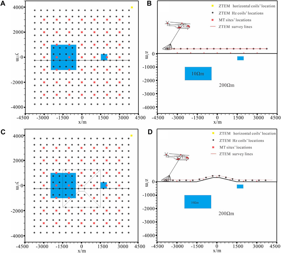
FIGURE 1. Survey grids for the synthetic models. (A) Synthetic model without topography on xy plane; (B) synthetic model without topography on yz plane; (C) synthetic model with topography on xy plane; (D) synthetic model with topography on yz plane. The three grids are MT sites (red squares), ZTEM sites (black circles), and ZTEM base site (yellow square).

The ZTEM vertical magnetic fields at frequencies of 30, 45, 90, 180, 360, and 720 Hz were computed both at a fixed altitude of 100 m over the plat and for a quadrangular platform Earth surface. To complement the ZTEM survey, the MT survey data of 0.04, 0.1, 0.4, 1, 3.5, 7, 45, 70, 90, 180, and 360 Hz were simulated. We used TetGen (Si, 2013) to generate the unstructured tetrahedral grids. As shown in Figure 2A, the computational domain for the model without topography was discretized into 272,798 elements for the forward modeling, while for the inversion in Figure 2A we divided the model into 265,981 elements. As shown in Figure 2C, the computational domain for the model with topography was discretized into 471,203 elements for the forward modeling, while for the inversion in Figure 2D we divided the model into 487,828 elements. We added 2% Gaussian noise to the synthetic ZTEM transfer functions tipper data MT and impedance data and set ${\epsilon }_n$ in Eq. 12 to 0.002 for ZTEM and 2% times |ZxyZyx|^1/2 for MT, respectively. Both the initial and reference models for the inversions were chosen to be a half-space as in Figures 2B,D with a given resistivity. Determining a reasonable starting model is critical for any inversion. We chose different resistivities of the initial models for four different test inversions, as shown in Table 2, to evaluate our joint inversions.

FIGURE 2

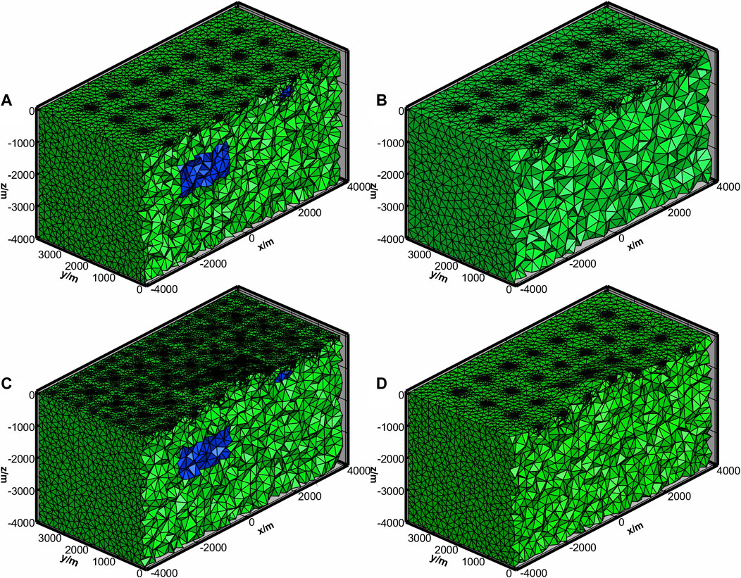
FIGURE 2. Model discretization for (A) forward modeling without topography, (B) inversion without topography, (C) forward modeling with topography, and (D) inversion without topography.

TABLE 2

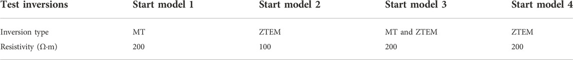
TABLE 2. Initial model settings.

Figures 3, 4 show the slices of the results from our test inversions on the horizontal and vertical planes, respectively. The rectangles indicate the outlines of the anomalous bodies. The results of the MT inversions with and without topography for start model 1 shown in Figures 3A, 4A, 5A, 6A only recover the lower conductive body but have a poor revolution for the shallow small body. This is expected, as MT is used with site intervals and lower frequency. For this reason, MT is mainly used to study the conductivities of large and deep structures in the Earth. Start model 3 uses an accurate initial model. The results of the ZTEM inversion for start model 2 in Figures 3B, 4B, 5B, and 6B recovered the shallow body and deep body. However, the deep body is vertically compressed compared to the real model, indicating that ZTEM has a poor resolution for deep structures below 1,500 m. As ZTEM is sensitive to upper structures, which have significant relative resistivity to the background medium [2–3], traditional methods that are used to determine a best-fitting half-space resistivity model cannot be used for ZTEM inversion. Start model 1 and start model 3 use inaccurate initial models. The results of the joint inversion in Figures 3C, 4C, 5C, 6C for Model 3 show that the joint inversion recovers both bodies. In addition, the recovered resistivities of the abnormal bodies and the background are approximate to those of the real model. This indicates that combining coarse MT and ZTEM inversion is effective in alleviating the shortcomings of the single MT and ZTEM inversion and has improved the model in the near-surface and at depth. The results of the ZTMT inversion for start model 4 in Figures 3D, 4D, 5D, 6D also recover anomalies with relatively correct positions. However, the lower part of the true body is not clearly displayed in the case without topography. As a comparison, the lower part of the true body is lost for the case with topography, as topography adds the depth of the deep structure. Comparing start model 2 and start model 4, it can be found that ZTEM inversion can give a reasonable resistivity model only when the initial models are close to the real background, while joint inversion does not depend on an accurate initial model and eliminates the redundant structures in ZTEM inversion. At the same time, joint inversion can combine the advantages of MT and ZTEM, which can provide a good revolution on shallow and deep structures.

FIGURE 3

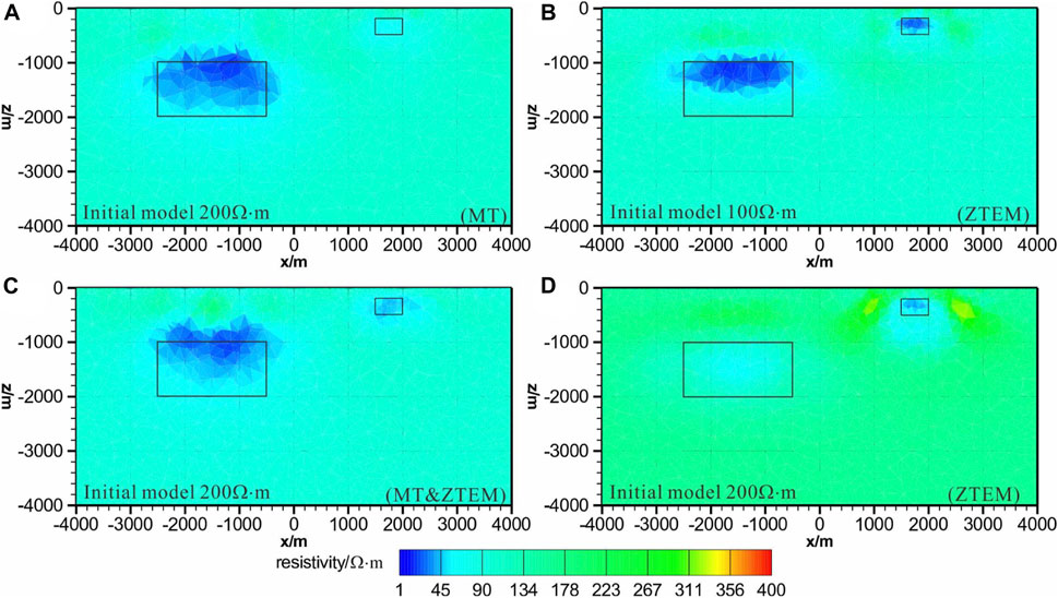
FIGURE 3. Inversion results for the synthetic model without topography respectively at the xz section for y=0 m. (A,D) and (C) are MT inversion, ZTEM inversion, and joint MT and ZTEM inversion with initial model and a 200 Ω·m half-space, respectively. (B) is the ZTEM inversion with a 100 Ω·m half-space.

FIGURE 4

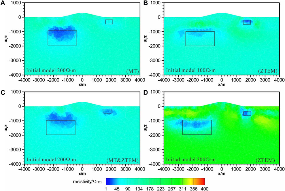
FIGURE 4. Inversion results for the synthetic model with topography at the xz section for y=0 m. (A,D) and (C) are the MT inversion, ZTEM inversion, and joint MT and ZTEM inversion with initial model and a 200 Ω·m half-space, respectively. (B) is the ZTEM inversion with a 100 Ω·m half-space.

FIGURE 5

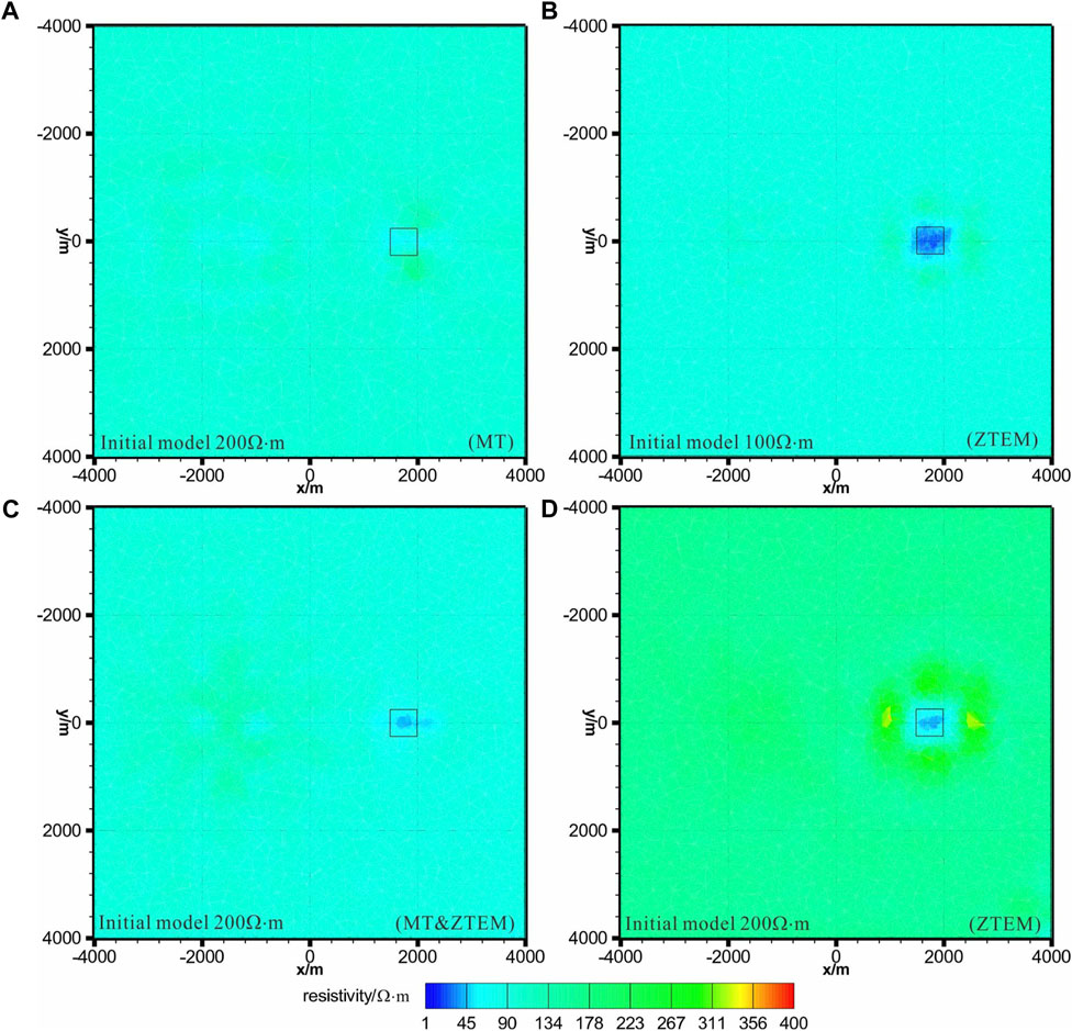
FIGURE 5. Inversion results for the synthetic model without topography at xy section for z=−450 m. (A,D) and (C) are the MT inversion, ZTEM inversion, and joint MT and ZTEM inversion with initial model and a 200 Ω·m half-space, respectively. (B) is the ZTEM inversion with a 100 Ω·m half-space.

FIGURE 6

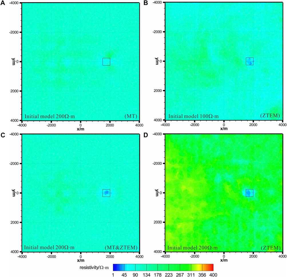
FIGURE 6. Inversion results for the synthetic model with topography at xy section for z=−450 m. (A,D) and (C) are the MT inversion, ZTEM inversion, and joint MT and ZTEM inversion with initial model and a 200 Ω·m half-space, respectively. (B) is the ZTEM inversion with a 100 Ω·m half-space.

Figure 7A shows that the fastest convergence of the model without topography is the ZTEM inversion with an accurate initial model. The slowest convergence is the MT inversion with an inaccurate initial model of 200 Ω·m. The convergence of an accurate initial model for ZTEM is faster than the inexact model inversion with 200 iterations, and it is similar to that of the model with topography in Figure 7B. This indicates that different initial models can result in variations in inversion result models, even if the data are sufficiently fit. The convergence of the joint inversion is between the MT and ZTEM, even if the initial model is inexact. Figures 7C,D show ${\phi }_r$ to increase rapidly at first and finally to decrease slightly to convergence for all inversions, with and without topography. For the ZTEM inversions with and without topography, ${\phi }_r$ converges to approximately the same value. At the same time, for MT inversions and joint ZTEM and MT inversion without topography, ${\phi }_r$ converges to approximately the same value. For MT inversions and joint ZTEM and MT inversion with topography, ${\phi }_r$ converges to a larger value for MT inversion than the joint inversion. Figures 7E,F show ${\phi }_s$ to converge to different values for inversions with and without topography. In general, ${\phi }_s$ for inversions with topography are greater than without topography.

FIGURE 7

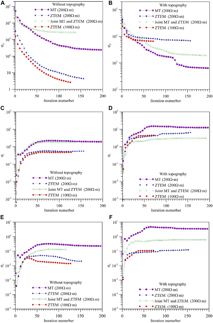
FIGURE 7. (A,B) Data misfit ${\phi }_d$, (C,D) model roughness measures ${\phi }_r$, and (E,F) smallness measures ${\phi }_s$ versus iterations.

4.2 Synthetic data inversion with topography

In this section, we demonstrate the effectiveness of our joint inversion algorithm for a topographical Earth, as shown in Figure 8. The elevation varies from 230 m to −10 m (Figure 6A). Referring to Figures 8A,B, the model consists of an Earth with a conductive body and a resistive body embedded. The half-space has a resistivity of 100 Ω·m. The conductive body has a resistivity of 10 Ω·m with dimensions of 2000 m × 2000 m × 1,000 m, respectively, in the x-, y-, and z-directions. The center of the conductive body is located at (1,500 m, 0 m, 750 m). The resistive body has a resistivity of 500 Ω·m with dimensions of 2000 m × 2000 m × 1,000 m, respectively, in the x-, y-, and z-directions. The center of the conductive body is located at (−1,500 m, 0 m, 750 m). The ZTEM vertical magnetic fields at frequencies of 30, 45, 90, 180, 360, and 720 Hz are computed at a fixed altitude of 100 m over the topographical surface. In addition, the MT survey data of 0.04, 0.1, 0.4, 1, 3.5, 7, 45, 70, 90, 180, and 360 Hz are simulated. Three different survey configurations over an 8 km × 8 km area were used, as shown in Figure 8A. The first survey has sparse MT stations, with only five stations, with 3-km station and line intervals, which could not be used for any 3D exploration projects due to their poor resolution. The second survey is a finer MT survey with 49 stations on the topographical surface in total, with 1-km station and line intervals. The third survey is a fine ZTEM survey with 256 stations (ZTEM Hz coils’ locations) at a fixed altitude of 100 m over the total topographical surface, with 500-m station and line intervals. The horizontal magnetic fields are calculated at a ground-based reference station (ZTEM horizontal coil location) located at x=3,750 m, y=3,750 m.

FIGURE 8

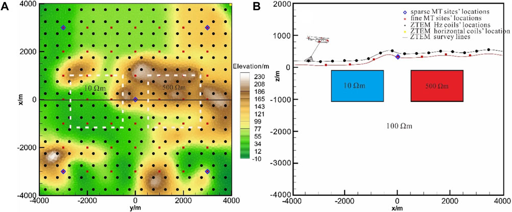
FIGURE 8. Survey grids for the synthetic model. The three grids are coarse MT (red squares), fine MT (blue diamonds), and ZTEM (black circles). The blue square is the ZTEM base.

Since the ZTEM data are very sensitive to topography, it is important to finely discretize them. The computational domain was discretized into 414,394 elements for the forward modeling (Figure 9). We added the Gaussian noise, as in the previous section, to the synthetic ZTEM transfer functions tipper data and MT impedance data before inversion. Both the initial and reference models for the inversions were chosen to be a half-space, which was divided into 362,745 elements with the same topography as Figure 9A. Four inversions with different initial model and survey configurations were tested, as shown in Table 3. Start model 1 is a ZTEM inversion with a 200 Ω·m initial model. Start model 2 is a ZTEM inversion with a 100 Ω·m initial model. Start model 3 is the joint MT and ZTEM inversion with the sparse MT survey and a 200 Ω·m initial model. Start model 4 is the joint MT and ZTEM inversion with the fine MT survey and a 200 Ω·m initial model.

FIGURE 9

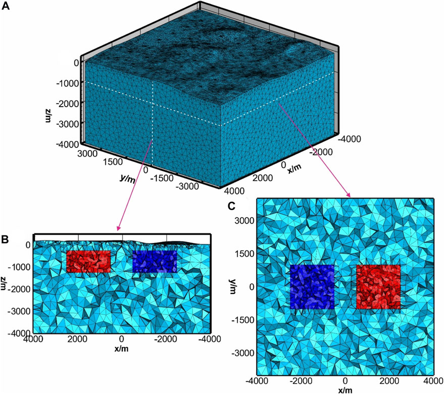
FIGURE 9. Model discretization for the forward modeling. (A) 3-D view of the models. (B) Side view of the model (y=0 m). (C) Plane view of the model (z=−1100 m).

TABLE 3

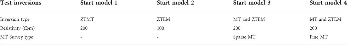
TABLE 3. Inversion settings.

Figures 10, 11 show the slices of the results of the four test inversions at the xz-section for y=0 m and the xy-section for z=−500 m. The rectangles indicate the outline of the true abnormal bodies. In Figures 8A, 9A for start model 1, the average resistivities for the revealed anomalous bodies and the background were higher than the real model. The inversion depth for the resistive body is beyond the real model, as shown in Figure 8A, while the conductive body has low resolution. In contrast, as shown in Figures 10B, 11B for start model 2, the average resistivities for revealed anomalous bodies and the background approximate the real model, which indicates that single-ZTEM inversion depends on an adequate initial model, like the first synthetic data inversion in the previous section. The inversion depth for the conductive body is lower than in the real model, as shown in Figure 10B, and the conductive body has good resolution, as shown in Figure 11B. In Figures 10C, 11C for start model 3, the average resistivities for the revealed anomalous conductive body and the background approximate the real model, but the resistive body also has a moderate resolution. In Figures 10D and 11D for start model 4, the average resistivities for the revealed anomalous conductive and resistive bodies and the background approximate the real model, and the resistive body has good resolution, which indicates that adding MT data calibrates the resistivity of ZTEM inversion. However, that of the sparse MT survey is much higher than the real model. As expected, the inverted depth of Model 4 for the fine MT survey is much lower, nearly the same as the real model; by increasing the number of MT stations, the shapes of the anomaly bodies are better resolved. Models 3 and 4 indicate that adding MT data, even if a sparse MT survey is used, can calibrate the resistivities of ZTEM inversion, and MT data can increase the detection depth of ZTEM inversion.

FIGURE 10

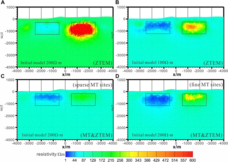
FIGURE 10. Inversion results for the synthetic model at the xz section for y=0 m. (A,B) and (C) are the MT inversion, ZTEM inversion, and joint MT and ZTEM inversion with initial model and a 200 Ω·m half-space, respectively. (D) is the ZTEM inversion with a 100 Ω·m half-space.

FIGURE 11

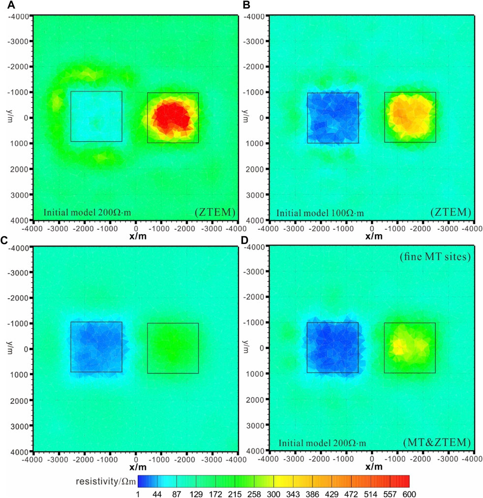
FIGURE 11. Inversion results for the synthetic model at the xy section for z=500 m. (A,B) and (C) are the MT inversion, ZTEM inversion, and joint MT and ZTEM inversion with initial model and a 200 Ω·m half-space, respectively. (D) is the ZTEM inversion with a 100 Ω·m half-space.

Figure 12A shows that ${\phi }_d$ decreases during the iterations for four start model inversions, which shows that the joint inversions converge faster than a single ZTEM inversion; however, the single ZTEM inversion with an inadequate initial model converges the slowest. Figures 12B and C show how the ${\phi }_r$ and ${\phi }_s$ change during convergence. Overall, ${\phi }_r$ increases sharply at first then increases slowly, finally decreasing slowly to convergence. For the joint inversions and the single ZTEM inversion with an adequate initial model, ${\phi }_s$ increases sharply at first, then increases steadily before a slight decrease and finally decreases to convergence with a once small increase. However, the single ZTEM with the inadequate initial model increases sharply first, then decreases significantly before increasing to the maximum and finally decreasing to convergence. Figure 12 indicates that the L-BFGS inversions are stable and convergent even with the condition of the topography and adequate initial model and the addition of spare MT data can improve the ZTEM inversion.

FIGURE 12

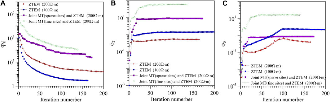
FIGURE 12. (A) Data misfit ${\phi }_d$, (B) model roughness measures ${\phi }_r$, and (C) smallness measures ${\phi }_s$ versus iterations.

6 Conclusion

In this study, based on the finite element method with unstructured tetrahedral grids and the L-BFGS method, we successfully developed a 3D inversion framework for joint MT and ZTEM data with topography. The unstructured grids can simulate complex underground structures and rugged topography, while the L-BFGS method avoids storing a large matrix; thus, the method is suitable for large-scale 3D MT and ZTEM inversions for complex geologies. An adequate MT survey, which may be inadequate for many exploration projects, can significantly enhance ZTEM inversion and adds significant information about deep structures. Joint inversion of MT and ZTEM data is a typical example of using the complementarity of ground and airborne EM data. Both synthetic data inversions verified the effectiveness of our algorithm. The inversion results showed that joint MT and ZTEM inversion can recover deep structures from the MT data and fine near-surface structures from the ZTEM data by alleviating the weaknesses of the individual methods, which calibrates the resistivities, rendering a correct a priori model unnecessary.

Data availability statement

The raw data supporting the conclusion of this article will be made available by the authors, without undue reservation.

Author contributions

Conceptualization, XC and XH; methodology, XC; investigation, XH; supervision, LY; project administration, JL; funding acquisition, FB. All authors have read and agreed to the submitted version of the manuscript.

Funding

This work was supported in part by the National Natural Science Foundation of China under Grant 42004053, Grant 42030805, Grant 42104070 and Grant 42274103, in part by the Fund from the Key Laboratory of Geophysical Electromagnetic Probing Technologies of Ministry of Natural Resources (KLGEPT202204) and in part by the Science and Technology Research Project of Sinopec Group, under Grant P22163.

Conflict of interest

The authors declare that the research was conducted in the absence of any commercial or financial relationships that could be construed as a potential conflict of interest.

Publisher’s note

All claims expressed in this article are solely those of the authors and do not necessarily represent those of their affiliated organizations, or those of the publisher, the editors, and the reviewers. Any product that may be evaluated in this article, or claim that may be made by its manufacturer, is not guaranteed or endorsed by the publisher.

References

Cao, X. Y., Huang, X., Yin, C. C., Yan, L. J., and Han, Y. Q. (2022). 3-D inversion of Z-axis tipper electromagnetic data using finite-element method with unstructured tetrahedral grids. IEEE Trans. Geosci. Remote Sens. 60, 1–11. doi:10.1109/tgrs.2021.3077510

CrossRef Full Text | Google Scholar

Cao, X. Y., Yin, C. C., Zhang, B., Huang, X., Liu, Y., and Cai, J. (2018). 3D magnetotelluric inversions with unstructured finite-element and limited-memory quasi-Newton methods. Appl. Geophys. 15 (3-4), 556–565. doi:10.1007/s11770-018-0703-8

CrossRef Full Text | Google Scholar

Cao, X. Y., Yin, C. C., Zhang, B., Huang, X., Liu, Y., and Cai, J. (2018). A Goal-oriented adaptive finite-element method for the 3D MT anisotropic modeling with topography. Chin. J. Geophys. (In Chin. 61 (6), 2618. doi:10.6038/cjg2018L0068

CrossRef Full Text | Google Scholar

Haldar, S. K. (2013). Mineral exploration: Principles and applications. Elsevier.Amsterdam, Netherlands

Google Scholar

Holtham, E. M. (2012). 3D inversion of natural source electromagnetic data. PHD thesis. London, UK: The University of British Columbia.

Google Scholar

Holtham, E., and Oldenburg, D. W. (2010). Three-dimensional inversion of ZTEM data. Geophys. J. R. Astronomical Soc. 182 (1), 168–182.

CrossRef Full Text | Google Scholar

Jahandari, H., and Farquharson, C. G. (2017). 3-D minimum-structure inversion of magnetotelluric data using the finite-element method and tetrahedral grids. Geophys. J. Int. 211 (2), 1189–1205. doi:10.1093/gji/ggx358

CrossRef Full Text | Google Scholar

Jin, J. (2014). The finite element method in electromagnetics. Wiley-IEEE Press.Hoboken, NJ, USA.

Google Scholar

Kaminski, V., Sattel, D., and Witherly, K. (2012). The effect of topography on ZTEM inversions.” in Proceedings of the 74th EAGE Conference and Exhibition.Copenhagen, Denmark.

CrossRef Full Text | Google Scholar

Legault, J., Kumar, H., Milicevic, B., and Wannamaker, P. (2009). ZTEM tipper AFMAG and 2D inversion results over an unconformity uranium target in northern Saskatchewan. Houston, TX, USA: Seg Technical Program Expanded.

Google Scholar

Legault, J. M. (2012). Ten years of passive airborne AFMAG EM development for mineral exploration: 82nd international exposition and annual meeting. Expanded Abstracts.Houston, TX, USA: SEG.

Google Scholar

Legault, J., Wilson, G. A., Gribenko, A. V., Zhdanov, M. S., Zhao, S., and Fisk, K. (2012). An overview of the ZTEM and AirMt airborne electromagnetic systems: A case study from the nebo-babel Ni-Cu-pge deposit, west musgrave, western Australia. Preview 2012 (158), 26–32. doi:10.1071/pvv2012n158p26

CrossRef Full Text | Google Scholar

Liu, D. C., and Nocedal, J. (1989). On the limited memory BFGS method for large scale optimization. Math. Program. 45 (1), 503–528. doi:10.1007/bf01589116

CrossRef Full Text | Google Scholar

Lo, B., and Zang, M. (2008). Numerical modeling of Z-TEM (airborne AFMAG) responses to guide exploration strategies. Seg. Tech. Program Expand. Abstr. 27 (1), 1098. doi:10.1190/1.3059115

CrossRef Full Text | Google Scholar

Newman, G. A., and Alumbaugh, D. L. (2010). Three-dimensional magnetotelluric inversion using non-linear conjugate gradients. Geophys. J. Int. 140 (2), 410–424. doi:10.1046/j.1365-246x.2000.00007.x

CrossRef Full Text | Google Scholar

Nocedal, J. (1980). Updating quasi-Newton matrices with limited storage. Math. Comput. 35 (151), 773–782. doi:10.1090/s0025-5718-1980-0572855-7

CrossRef Full Text | Google Scholar

Ren, Z., Kalscheuer, T., Greenhalgh, S., and Maurer, H. (2013). A goal-oriented adaptive finite-element approach for plane wave 3-D electromagnetic modelling. Geophys. J. Int. 194 (2), 700–718. doi:10.1093/gji/ggt154

CrossRef Full Text | Google Scholar

Sampson, L. M., and Williams, N. C. (2021). The geophysical response of the Goldrush-Fourmile orebody and implications for camp-scale Carlin-type deposit exploration, Cortez District, Nevada. Lead. Edge 40 (2), 122–128. doi:10.1190/tle40020122.1

CrossRef Full Text | Google Scholar

Sasaki, Y., Yi, M. J., and Choi, J. (2014). 2D and 3D separate and joint inversion of airborne ZTEM and ground AMT data: Synthetic model studies. J. Appl. Geophys. 104, 149–155. doi:10.1016/j.jappgeo.2014.02.017

CrossRef Full Text | Google Scholar

Sattel, D., Witherly, K., and Kaminski, V. (2019). A brief analysis of MobileMT data. 89th Annu. Int. Meet. Seg. Expand. Abstr., 2138. doi:10.1190/segam2019-3215437.1

CrossRef Full Text | Google Scholar

Sattel, D., and Witherly, K. (2021). The joint inversion of active-source and natural-field EM data. Proceedings of the 1st International Meeting for Applied Geoscience and Energy.Denver, Colorado.

Google Scholar

Si, H. (2013). TetGen a quality tetrahedral mesh generator and a 3D Delaunay triangulator. Berlin, Germany: Weierstrass Institute for Applied Analysis and Stochastics.

Google Scholar

Smiarowski, A., and Konieczny, G. (2019). Low-base frequency helicopter AEM data from a square-wave system – Helitem2. ASEG Ext. Abstr. 1, 1–5. doi:10.1080/22020586.2019.12073153

CrossRef Full Text | Google Scholar

Soyer, W., and Mackie, R. L. (2018). Comparative analysis and joint inversion of MT and ZTEM data. ASEG Ext. Abstr. 1, 1–7. doi:10.1071/aseg2018abt5_2f

CrossRef Full Text | Google Scholar

Tikhonov, A. N., and Arsenin, V. Y. (1977). Solutions of ill-posed problems. Hoboken, NJ, USA: Wiley.

Google Scholar

Wang, F., Petter, M. J., and Klaus, S. (2018). Anisotropic three-dimensional inversion of CSEM data using finite-element techniques on unstructured grids. Geophys. J. Int. 213 (2), 1056–1072. doi:10.1093/gji/ggy029

CrossRef Full Text | Google Scholar