 Matteo Ravasi
- Physical Science and Engineering, King Abdullah University of Science and Technology, Thuwal, Saudi Arabia
Seismic data processing heavily relies on the solution of physics-driven inverse problems. In the presence of unfavourable data acquisition conditions (e.g., regular or irregular coarse sampling of sources and/or receivers), the underlying inverse problem becomes very ill-posed and prior information is required to obtain a satisfactory solution. Sparsity-promoting inversion, coupled with fixed-basis sparsifying transforms, represent the go-to approach for many processing tasks due to its simplicity of implementation and proven successful application in a variety of acquisition scenarios. Nevertheless, such transforms rely on the assumption that seismic data can be represented as a linear combination of a finite number of basis functions. Such an assumption may not always be fulfilled, thus producing sub-optimal solutions. Leveraging the ability of deep neural networks to find compact representations of complex, multi-dimensional vector spaces, we propose to train an AutoEncoder network to learn a nonlinear mapping between the input seismic data and a representative latent manifold. The trained decoder is subsequently used as a nonlinear preconditioner for the solution of the physics-driven inverse problem at hand. Through synthetic and field data examples, the proposed nonlinear, learned transformations are shown to outperform fixed-basis transforms and converge faster to the sought solution for a variety of seismic processing tasks, ranging from deghosting to wavefield separation with both regularly and irregularly subsampled data.
1 Introduction
Geophysical inverse problems are notoriously ill-posed and ad-hoc regularisation techniques are usually employed to produce solutions that satisfy our available prior knowledge. A typical example in seismic processing is represented by the problem of seismic data interpolation where data acquired by sparsely sampled arrays of receivers are reconstructed onto a regular, finely sampled grid of choice.
Interpolation methods can be divided into four main categories: spatial Prediction-Error-Filters (PEFs), wave-equation based, rank-reduction, and domain transform. PEFs interpolation methods (Spitz, 1991; Liu and Fomel, 2011) locally represent seismic data as a superposition of a small number of plane waves; such methods reconstruct aliased data by exploiting their non-aliased low-frequency components. Wave-equation based algorithms (Ronen, 1987; Fomel, 2003), on the other hand, fill gaps in the data by means of an implicit migration-demigration scheme. Transform-based algorithms (Trad et al., 2002) exploit the fact that seismic data can be represented by a small number of non-zero coefficients in a suitable transformed domain, whilst acquisition gaps introduce noise in such a domain. Reconstructing missing traces therefore becomes a denoising problem in the transformed domain, which can be tackled by means of direct filtering or sparsity-promoting inversion (Hennenfent and Herrmann, 2008). In the latter case, the Lp norm (p ≤ 1) of the reconstructed seismic data in the transformed domain is minimized whilst matching the available traces. The frequency-wavenumber (F-K) transform (Abma and Kabir, 2006; Schonewille et al., 2009), Radon transform (Kabir and Verschuur, 1995; Sacchi and Ulrych, 1995), and Curvelet-like transforms (Herrmann and Hennenfent, 2008; Fomel and Liu, 2010; Hauser and Ma, 2012) are examples of successful fixed-basis sparsifying transforms. Alternatively, data-driven sparse dictionaries can be learned directly from the dataset at hand (Zhu et al., 2017). Nevertheless, the success of this family of methods is partially hindered by the slow convergence of most sparsity-promoting optimizers and by the fact that weaker events are usually poorly reconstructed. Finally, rank-reduction methods (Trickett et al., 2010; Oropeza and Sacchi, 2011; Kumar et al., 2012; Yang et al., 2013) lie their foundation on the observation that fully sampled seismic data exhibit a low-rank pattern that is deteriorated when irregular gaps are introduced in the data. This approach is the generalization of the sparsity-based inversion to matrices, in that minimizing the nuclear norm of a matrix is equivalent to minimizing the L1 norm of a vector containing its eigenvalues.
Despite its enormous popularity, interpolation alone is seldom of interest during a seismic processing project. Combining multiple processing steps into a single inversion is in fact likely to reduce the propagation of errors from one step of processing to the next and increase the processing turnaround time. Being based on the solution of an inverse problem, rank-reduction and transform-based algorithms lend nicely to the introduction of additional physical constraints to further mitigate the ill-posed nature of the seismic interpolation problem. For example, by separating the recorded data into its up- and down-going components as part of the interpolation process, an explicit ghost model can be introduced to provide further physical constraints to the sought solution. Such a strategy can be employed when using either single-sensor data (Grion, 2017) or multi-sensor data (Ozbek et al., 2010). Similarly, when receiver-side gradients of the recorded wavefield are also available, additional data terms can be easily included in the problem improving the capabilities of the reconstruction process far beyond the Nyquist sampling criterion (Vassallo et al., 2010; Ruan and Vasconcelos, 2019).
The success of deep learning in various scientific disciplines has recently gained the attention of the geophysical community. Encouraging applications of deep learning in various seismic processing and interpretation tasks have been reported, ranging from denoising (Saad and Chen, 2020; Yu et al., 2021; Birnie and Alkhalifah, 2022), deblending (Richardson and Feller, 2019; Sun et al., 2020; Luiken et al., 2022), velocity analysis (Yang and Ma, 2019; Sun et al., 2020; Kazei et al., 2021), fault and geobodies interpretation (Waldeland et al., 2018; Shi et al., 2019; Wu et al., 2020), to reservoir characterization (Zhao, 2018; Alfarraj and AlRegib, 2019; Das et al., 2019). We refer the reader to Yu and Ma (2021) for an exhaustive literature review on the topic. A new family of methods that leverage neural networks within the context of seismic interpolation has also emerged: Mandelli et al. (2019) recast the data reconstruction problem as an end-to-end learning task and use the popular U-Net architecture to learn a mapping between the sparsely sampled and fully sampled seismic data. Similarly, Siahkoohi et al. (2018) suggest to use conditional adversarial networks by augmenting the learning process with a discriminator network following the Image-to-Image translation framework of Isola et al. (2017). More recently, Kuijpers et al. (2021) and Vasconcelos et al. (2022) leverage Recurrent Inference Machines (RIMs), a special type of learned iterative solver (Adler and Oktem, 2017) that is specifically designed to solve inverse problems in a data-driven fashion, whilst still including prior knowledge about the forward operator. Such an approach has been shown to outperform end-to-end supervised learning methods and better generalize to out-of-distribution data in various applications including MRI reconstruction (Lønning et al., 2019) and imaging of gravitational lenses (Morningstar et al., 2019), to cite a few.
Nevertheless, all of the aforementioned approaches share the same limitation: they require representative pairs of decimated and fully sampled data, which is usually not available in most seismic processing projects. Whilst relying on synthetic data or field data with similar characteristics (e.g., from nearby survey) may alleviate the arising of generalization issues, the trained network is usually expected to perform sub-optimally at test time when applied to a different dataset. We refer to Mandelli et al. (2019) for an in-depth analysis of the generalization issues of supervised learning approaches in the context of seismic data reconstruction. So-called domain adaptation techniques (e.g., Alkhalifah et al., 2021; Birnie and Alkhalifah, 2022) may provide a remedy to this problem; however, such generalization issues have also motivated the development of a second wave of deep learning based algorithms that use neural networks in combination with the known physics of the problem to drive the solution of the inverse problem towards physically plausible solutions. Along these lines, Kong et al. (2020) propose to solve the seismic reconstruction problem in an unsupervised manner using an untrained network as a deep prior preconditioner following the Deep Image Prior concept introduced in Ulyanov et al. (2017). Whilst this approach circumvents the need for any training data, it is currently hindered by very slow convergence and it is shown to be incapable of recovering strongly aliased events. Anti-aliasing, slope-based regularization (Picetti et al., 2021) or a POCS-inspired regularization (Park et al., 2020) have been further proposed to increase the interpolation capabilities of such deep prior networks.
Following a different line of thought, Li et al. (2020) suggests to train a nonlinear dimensionality reduction model, such as an AutoEncoder network (AE—Kramer, 1991), in order to identify latent representations of the expected solution manifold. In a subsequent step, the pre-trained network is used as a regularizer in the solution of a physics-driven inverse problem in the medical imaging context. Obmann et al. (2020) have extended this procedure to sparse AEs and modified the regularization term of the inverse problem to penalize solutions that do not belong to the manifold. Whilst this approach closely resembles classical sparsity promoting inversion schemes with over-complete linear basis functions and provides some theoretical guarantees, it usually renders a more challenging training and inversion compared to the original method. In concurrent work, Ravasi (2021) proposed to use the decoder of the trained AE as a nonlinear preconditioners, solving the inverse problem directly in the latent space of the network. This naturally enforces solutions to be consistent with the manifold of the training data and does not require finding a good balance between the data misfit term and the regularization term. To remark the fact that this preconditioner is composed of a neural network, this approach will be referred to herein as Deep Preconditioner.
In this work, we further develop the approach of Ravasi (2021) and show that by carefully designing the AE network architecture, loss function, and the pre-processing pipeline associated with the training data, strong representations can be obtained that ultimately improve the quality of the downstream inversion task. We showcase various applications, ranging from deghosting to wavefield separation with both regularly and irregularly subsampled data, applying them to synthetic datasets of increasing complexity and a marine field dataset. Both the deghosting and wavefield separation modelling operators will be introduced in details in the Numerical examples section. Finally, we notice that contrary to medical applications where a set of representative models is usually available upfront, this is not always the case in seismic applications: we show that a representative latent manifold can nevertheless be identified using data that are not exactly in the same form of the model we wish to invert for. For example, in the problem of joint deghosting and data reconstruction, the AE is trained on the available ghosted data whilst the learned decoder is used to invert the recorded data for a finely sampled, deghosted data.
The paper is organized as follows. In Section 2, we introduce the theory of Deep Preconditioners and the training process of the associated AE network. In Section 3, we first apply the proposed approach to a toy problem of one-dimensional signal reconstruction. Subsequently, the same approach is used to solve the joint deghosting and seismic data reconstruction as well as the joint wavefield separation and interpolation problems. In Section 4, we discuss a number of avenues for future research, whilst some conclusive remarks are presented in Section 5.
2 Theory
An inverse problem is the process of estimating from a given set of observations the unknown underlying factors that originated them. Due to their ill-posed nature, geophysical inverse problems cannot be solved relying on the observations alone, instead additional prior knowledge is also required; such information can be provided either in the form of regularization or preconditioning. In this section, we first recap some basic concepts of the theory of regularized inverse problems. Second, we introduce nonlinear, learned regularizers and preconditioners and discuss how to interchange them with their more commonly used linear counterparts. Finally, the training process devised to learn strong latent representations from a collection of training data is described.
2.1 Introduction to inverse problems
In this work, we are concerned with finding a stable solution to a linear inverse problem of the form:
where
When the problem is well-posed, the solution of Eq. 1 can be obtained by simply inverting the modelling operator:
where R is the regularization operator and
Alternatively, a constrained inverse problem can be created to ensure that the sought after solutions satisfies certain conditions:
where
where
2.2 Deep regularization and preconditioning
In both of the approaches discussed so far, the choice of the regularizer and preconditioner is generally driven by experience and it can take a great deal of human effort and time to find a suitable transform for a specific problem. Whilst dictionary learning can partially overcome this limitation (Zhu et al., 2017), linear bases struggle to accurately approximate complex vector spaces such as those spanned by seismic data. This is however not the case for nonlinear dimensionality reduction techniques that leverage deep neural networks as we will see in the following.
To begin with, Eqs 2, 4 must be adapted to accommodate for such nonlinear transformations. Starting from the regularized inverse problem, Eq. 2 can be recast as (e.g., Obmann et al. (2020)):
Alternatively, the preconditioned inverse problem in Eq. 4 can be rewritten as (Ravasi, 2021):
where
2.3 AutoEncoder training
In both of the above scenarios, the solution of the inverse problem in Eqs 5, 6 is formulated as a two-steps process as depicted in Figure 1: first, an AE network is trained to learn a latent representation from a set of training data that share high-level features with the expected solution of the inverse problem at hand. Subsequently the entire network (in the regularized case) or the decoder part of the network (in the preconditioned case) is used to drive the solution of the inverse problem towards a solution that belongs to the manifold of the training data.
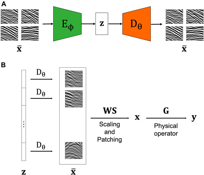
FIGURE 1. Schematic representation of the proposed two-step approach for the solution of geophysical inverse problems. (A) Training phase: an AE network is trained to reproduce patches of seismic data with the aim of learning robust latent representations. (B) Inversion phase: the pre-trained decoder is coupled to a physical modelling operator G to solve a geophysical inverse problem of choice. Note that since training has been performed using patches, the latent vector z is composed of a stack of latent codes from different patches of the model vector that we wish to reconstruct. Moreover, since during training all patches have been scaled between [−1, 1] an adaptive scaling operator S is applied to the different patches before combining them together via a patching operator W.
Starting from the training phase, this process is performed by using a training dataset of ns samples,
where
where
The training process of an AE network is usually impacted by the choice of the network architecture, loss function(s), and training data (and their associated pre-processing). In the subsequent subsections, we highlight a number of strategies that have been adopted in our numerical examples to enhance the reconstruction capabilities of the AE network, whilst ultimately producing more expressive latent representations. This will in turn impact the quality of our downstream task (e.g., deghosting and interpolation). As such, the effectiveness of the different training strategies will be evaluated both by computing the Mean Square Error
2.3.1 Network architecture
When dealing with gridded, multi-dimensional signals such as natural images or seismic data, Convolutional Neural Networks (CNNs) represent the most natural choice for the network architecture. Convolutional AEs (Masci et al., 2011) are usually composed of a number of convolutional layers followed by downsampling (implemented via average or max pooling) in the encoder (or contracting) path, and similarly by a number of convolutional layers followed by upsampling (implemented via, for example, bilinear interpolation) in the decoder (or expanding) path; moreover, a 1 × 1 convolutional layer or a dense layers may be used at the end of the encoder path and at the start of the decoder path to transform the convolutional features into a vector of size z (i.e., the latent code). Here, we use the latter choice of layer. A final convolutional layer is also added to the decoder to restore the number of channels to 1 like in the input data.
In this work, a purely convolutional network architecture is chosen as baseline (Figure 2A). Each block in the contracting and expanding paths is composed of two convolutional layers followed by batch normalization and a Leaky Rectified Linear Unit (or Leaky ReLU) activation function (with α = 0.2). A hyperbolic tangent (TanH) activation function is used for the dense layer in the encoding path to ensure boundness of the latent space, whilst a ReLU activation function is used for the dense layer in the decoding path. Max pooling with stride of 2 is used in the encoding path and bilinear interpolation with upsampling factor of 2 is chosen for the decoding path. Two additional network architectures are also considered: the first replaces all the convolutional blocks with residual blocks, or ResNet blocks (He et al. (2015)—Figure 2B), whilst the latter uses MultiRes blocks (Kong et al. (2020)—Figure 2C), which have shown promise in the context of deep image prior bases seismic interpolation.
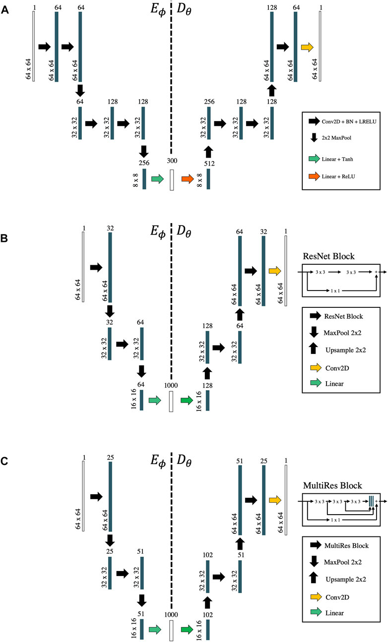
FIGURE 2. Network architectures. (A) Convolutional AE, (B) Convolutional AE with ResNet blocks, (C) Convolutional AE with MultiRes blocks.
2.3.2 Loss function
The choice of the loss function involved in the training process is usually dictated by the expected statistics of the noise present in the training data. More specifically, the MSE loss
where μx and σx are the mean and standard deviations of x, respectively (and similarly for the vector
In this work we follow this second strategy and combine the MSE and CCC losses together. Instead of choosing their relative weighting upfront, each loss is equipped with a learned weighting factor σi and defined as follows:
following the multi-task loss function proposed by Kendall et al. (2018). Intuitively σi quantifies the complexity associated with the ith task. The network is therefore naturally encouraged to learn the easy task first and tackle the harder task later. The network achieves this by initially increasing the weight of the loss associated to the hard task, which effectively reduces the contribution of the associated gradient into the minimization of the multi-objective functional. The network is however not allowed to completely ignore a task as that would require increasing the associated weight to infinity: this is avoided by the presence of the logarithmic term. Putting all together for our specific problem, the loss function in Eq. 8 becomes:
2.3.3 Pre-processing
In order to identify robust representations and avoid the network to learn the identity mapping, various regularization strategies have been proposed in the literature for training of AE networks. Denoising AEs (Vincent, 2008) partially corrupt the input vectors by adding noises to or masking some of their values in a stochastic manner. The target is however kept unchanged. This design is motivated by the fact that humans can easily recognize objects even when they are partially occluded or corrupted because they are able to focus on the key characteristic of such objects. Similarly, an AE can successfully learn robust latent representations only when it is forced to discover and capture high-level relationships in the input data whilst ignoring its missing parts. Since we are mostly interested in reconstructing missing gaps in seismic data as part of the downstream processing task, we follow the second procedure and randomly mask 20% of the traces from each training sample. This is done differently from epoch to epoch. This approach is becoming very popular in the machine learning community in the context of self-supervised learning for both text [e.g., Devlin et al. (2018)] and image [e.g., He et al. (2021)] analysis.
3 Numerical examples
3.1 Toy example: Reconstruction of one-dimensional sinusoidal signals
The proposed methodology is initially applied to a 1D, sinusoidal signal with the aim of interpolating irregularly spaced gaps in the data. Despite its apparent simplicity, this inverse problem is severely ill-posed and requires prior knowledge of the sought model vector in order to be able to fill the gaps in the recorded signal. This examples is therefore aimed at providing the reader with an intuitive understanding of the value of finding a suitable nonlinear latent representation of the model vector to solve problems in the form of Eq. 6. As a comparison we also solve the reconstruction problem with:
• a regularizer that penalizes the second-order derivative of the model (i.e., enforces smoothness) using Eq. 2;
• a preconditioner based on a linear dimensionality reduction technique using Eq. 4. Here, Principal Component Analysis (PCA—Hotelling, 1933) is chosen as the dimensionality reduction technique.
The forward problem is defined by a restriction operator that extracts values from the finely sampled signal
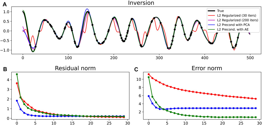
FIGURE 3. (A) Sinusoidal signal reconstruction for the different inversion approaches. (B) Residual norm and (C) error norm as function of iterations.
A major difference is also observed between the PCA and AE error norms: the former plateaus at around 2.5 after a few iterations, whilst the latter goes to zero after about 20 iterations. In other words, the latent representation found by means of PCA is not able to fully capture the signal we wish to recover, whilst that of the AE is more successful at mitigating the ill-posed nature of the inverse problem and drive the nonlinear optimizer to a satisfactory solution.
3.2 Seismic datasets
We turn now our attention onto the various seismic datasets that will be used in the subsequent numerical examples. The first synthetic dataset is modelled using a rather simple layered medium (Figure 4A) using a first-order, staggered-grid, acoustic finite-difference modelling code openly available in the Madagascar toolbox (Fomel et al., 2013). The acquisition geometry is composed of 201 sources spaced every 15 m at a depth of 10 m below the free-surface. Two receiver arrays are placed at a depth of 50 m below the free-surface and along a dipping seabed, respectively, both with receiver sampling equal to 15 m. The dataset is modelled using a Ricker wavelet with fdom = 15 Hz and two subsampled versions of it are created by decimating the receivers as follows: 1) irregularly, by a factor of 30%, or 2) regularly, by keeping one receiver every 4 (25% available data). A second synthetic dataset is created using a more realistic geological model obtained by adding a water column of 275 m to the Marmousi model (Brougois et al., 1990, Figure 4B). The acquisition geometry is composed of 199 sources spaced every 20 m at a depth of 10 m below the free-surface. A receiver array is placed at a depth of 50 m below the free-surface with receiver sampling equal to 20 m. The dataset is modelled using a Ricker wavelet with fdom = 15 Hz and also subsampled as follows: 1) irregularly by a factor of 40%, 2) regularly by keeping one receiver every 3 (33% available data). Finally, we consider the openly available Mobil AVO viking graben line 12 field dataset1. This dataset has been collected using streamer acquisition system that contains 1001 sources (dxS = 25m) and 120 receivers (dxR = 25m) with minimum offset equal to 262m. Sources and receivers are placed at a depth of 6 and 10 m below the free-surface, respectively. In our experiment, the dataset is further by randomly selecting 60% of the available receivers.
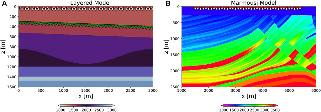
FIGURE 4. Velocity models. (A) Layered model with dipping seabed. Sources (red triangles) and receivers are placed inside the water column (white triangles) and along the seafloor (green triangles). (B) Marmousi model with sources and receivers located inside the water column.
3.3 AutoEncoder training
In this section, we discuss the training process of the AE network performed on the first synthetic dataset. To begin with, the dataset is sorted into common receiver gathers (CRGs) for all of the available receivers; overlapping patches of size 64 × 64 are created (a 50% overlap in both time and space is used in our experiments), and a data augmentation strategy is employed to increase the number of patches that contain events near the direct arrival; this is usually the arrival with largest slope and therefore exhibiting stronger aliasing effects in poorly sampled datasets. Here, we randomly select the center of the patch in a window around the traveltime of the direct arrival and each patch is also flipped horizontally to double the number of patches with similar characteristics. Each patch is also normalized by their absolute maximum value to ensure a maximum dynamic range of (−1, 1) for all of the available patches. As discussed in more details later in the paper, the main assumption made by our methodology is that we have access to well sampled seismic data in one domain of choice that is representative for the data in the poorly sampled domain. As seismic data are usually acquired in configurations where either the source or the receiver arrays are well sampled, exploiting reciprocity is a well known strategy, not only in this context but also in other traditional or data-driven (Picetti, 2022) seismic interpolation methods.
The entire dataset is composed of 30 k patches, which, similarly to the previous example, are randomly split into train (90%) and validation (10%) sets. Although the training process is fully unsupervised, the choice of retaining a number of patches for validation is motivated by the fact that we want to assess a variety of training strategies and compare them in terms of their reconstruction capabilities. The training process is performed using the Adam optimizer for 20 epochs, using an initial learning rate equal to 1e−4 in all experiments and modified during the training process using a scheduler: on-plateau scheduling is selected for the networks with single loss function, whilst the one-cycle scheduling (Smith and Topin, 2017) is chosen for the networks using multiple losses with learned weights. Finally, independent of the network architecture, the latent space vector is chosen as
Figures 5, 6 display four randomly selected patches from the validation dataset of the true and predicted data for the different training strategies, as discussed in the previous section. Moreover, the MSE over the entire validation dataset is reported in each subplot title. From these results, we can clearly observe an improvement in terms of the overall reconstruction capabilities when moving from a purely convolutional AE with single loss to an AE with ResNet blocks and multiple losses. On the one hand, a more sophisticated network architecture with MultiRes blocks led to poorer reconstruction and it is therefore dropped from subsequent analyses. Similarly, a slight decrease in the overall reconstruction error is observed when introducing the masking procedure in the pre-processing of each patch. However, as we will see later, the masking approach seems to help in producing stronger latent codes when it comes to the ultimate goal of using the trained decoder as preconditioners in the solution of different seismic data processing tasks.
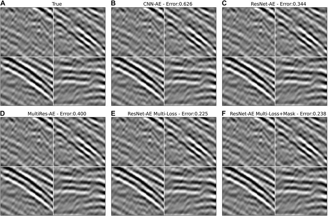
FIGURE 5. AutoEncoder reconstruction of 4 samples from the validation dataset and MSE computed over the entire validation dataset. (A) True, (B) Pure convolutional AE with MSE loss and no-preprocessing, (C) ResNet AE with MSE loss and no-preprocessing, (D) MultiRed AE with MSE loss and no-preprocessing, (E) ResNet AE with Multi-task loss and no-preprocessing, and (F) ResNet AE with Multi-task loss and masking of input samples.
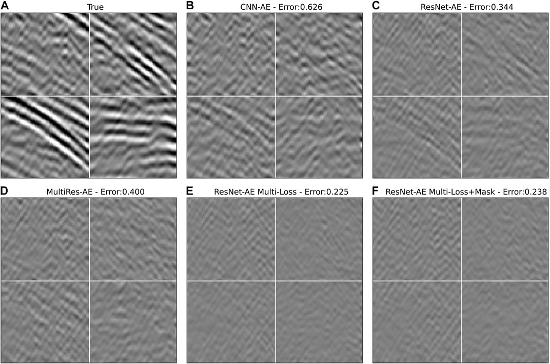
FIGURE 6. AutoEncoder reconstruction error of 4 samples from the validation dataset and MSE computed over the entire validation dataset. Panels are organized as Figure 5.
Finally, for the network in Figure 5F the latent representations of the entire validation dataset are further compressed to a bi-dimensional space using the t-SNE algorithm (Roweis and Hinton, 2002). This allows us to display them in a scatter plot as shown in Figure 7 and analyse how patches of the training seismic data with different features distribute in the latent space. Five points are selected in different areas and their associated patches are displayed inside blue squares. Similarly, patches in the validation data associated with the closest point in the bi-dimensional space are also displayed inside red squares. We can clearly observe how patches with similar features (e.g., high-amplitude hyperbolic events) cluster together. Finally a small random perturbation is added to the latent representations associated with the five selected patches and the resulting z vectors are fed into the trained decoder. The predicted patches are displayed inside the green squares. We can clearly observe that even areas of the latent space that have not been explored during training lead to representative seismic-looking patches. This is an important result as the subsequent inversion process will operate directly in the latent space and no constraint will be added to enforce the final latent vectors to be in any of the previously sampled positions of such a manifold.
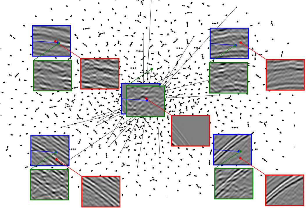
FIGURE 7. t-SNE visualization of the validation dataset in Figure 5F in a two-dimensional space. Seismic patches in blue, red, and green squares correspond to a number of selected validation samples, their closest neighbour and a perturbed version of it in the AE latent space, respectively.
3.4 Deghosting and interpolation of synthetic dataset
Joint receiver-side deghosting and data reconstruction is applied here to the first synthetic seismic dataset. The deghosting process can be described as an inverse problem by defining the following modelling operator [e.g., Grion, (2017)]:
where the model vector p− contains by the up-going component of the recorded seismic data, whilst the data vector p−d is represented the total pressure wavefield deprived of its direct wave. As far as the physical modelling operator is concerned, Φ represents a frequency-wavenumber phase shift operator and I is the identity operator. Combining this modelling operator with the definition of deep preconditioned inversion in Eq. 6, we obtain:
Since training is performed on patches of size 64 × 64, z is composed of a stack of multiple latent space vectors that are decoded by the decoder Dθ, re-scaled from the dynamical range of (−1, 1) used in the network to the actual range of the seismic data via the operator S, and finally assembled together by means of a patching operator W (Figure 1B). The scaling factors applied to each patch by the operator S are computed upfront from the corresponding patches in the data p−d: whilst these values may not correspond exactly to those of the sought solution, this choice revealed to be robust in all of the scenarios presented in this paper. Finally, the starting guess for the L-BFGS solver is here chosen as follows: z0 = Eϕ(S−1WHRHp−d). In other words, the recorded data is divided into patches, each patch is scaled to the dynamic range expected by the network by S−1, and then fed into the encoder.
Deghosting is initially applied to the fully sampled data (Figure 8A) for a source in the middle of the array (Figures 8C, 9B). The ill-posed nature of the problem, due to presence of notches in the F-K spectrum of the data (the first receiver ghost notch at fn1 = vwater/(2zr) = 15Hz is indicated by the white arrow in bottom panel of Figure 8A), is mitigated by using a preconditioned inversion with a Curvelet sparsifying transform. The FISTA solver (Beck and Teboulle, 2009) is used to optimize the associated functional for a total number of 200 iterations. This ensures that we accurately deghost the data also in areas with small amplitude events such that we can use this estimate as our benchmark solution. The subsampled data in Figures 8B, 9A are then inverted with fixed-basis sparsifying transforms, namely the F-K transform in overlapping time-space patches (Figures 8D, 9C) and the Curvelet transform (Figures 8E, 9D). Once again we use the FISTA solver for 80 iterations. Finally the trained decoder is used as preconditioner in Eq. 6, which is minimized with 80 iterations of L-BFGS (Figures 8F, 9E). Assuming that the cost of the linear transforms is similar to that of the decoder, setting the number of iterations to 80 for all inversions allows us to also compare the converge properties of the different algorithms. Both visually and by means of the SNR metric, we conclude that the AE-based inversion converges faster to produce results of higher quality compared to those from commonly used fixed-basis transforms. Visible artefacts in the solutions of the inversion methods that use linear preconditioners highlight the fact that such representations cannot capture the full complexity of the sought after seismic wavefield. Moreover, Figure 10 displays the SNRs of the reconstructed upgoing wavefields for the different training strategies discussed in the previous section. We observe how in both cases (irregular and regular), the vanilla CNN AE produces reconstructions on par with those from the sparse inversion with Curvelet transform. However, when the different improvements in the AE training process are introduced the overall SNRs improve by 2–3 dB compared to the initial scenario. Moreover, to verify that the initialization of the weights and biases of the network does not have a major impact in the overall quality of reconstruction of the downstream processing task, 5 networks are trained with different initialization and their different decoders are used to perform deghosting and interpolation. The standard deviation of the corresponding SNRs is displayed as a vertical black bar in Figure 10. Finally, to validate the importance of choosing a representative starting guess z0, the same deghosting and interpolation process is performed using randomly initialized vectors z0 (within the expected dynamic range of the latent code). The corresponding average and standard deviation SNRs are displayed as red bars in Figure 10, showing a clear decrease in performance likely due to the nonlinear nature of the inverse process and the fact that the starting guess is further away from the optimal solution compared to that using the proposed initialization strategy.
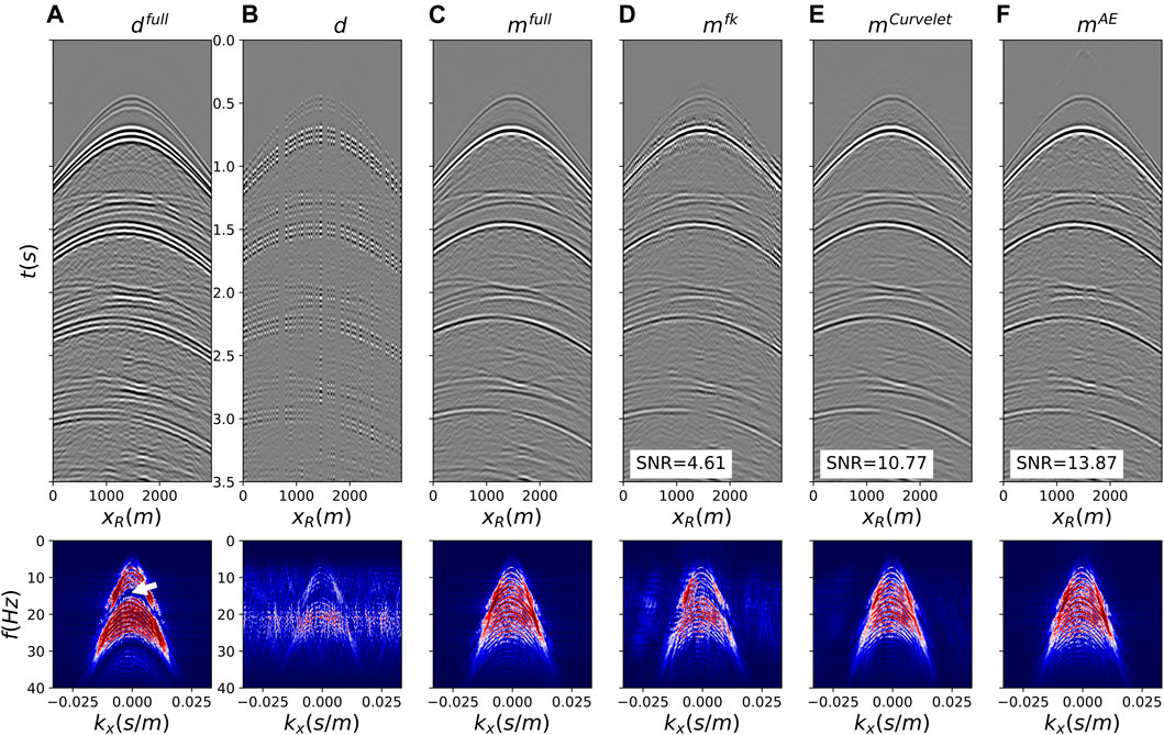
FIGURE 8. Joint deghosting and reconstruction for irregularly sampled data. (A) Full data, (B) Subsampled data, (C) Benchmark deghosted data, (E–G) Deghosted and reconstructed data using F-K, Curvelet, and AE preconditioners, respectively. All data are shown in time-space domain in the top row and frequency-wavenumber domain in the bottom row.
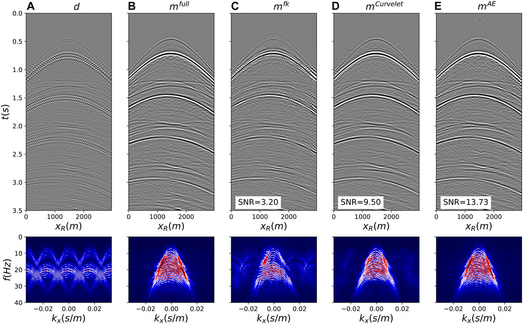
FIGURE 9. Joint deghosting and reconstruction from regularly sampled data. (A) Subsampled data, (B) Benchmark deghosted data, (C–E) Deghosted and reconstructed data using F-K, Curvelet, and AE preconditioners, respectively.
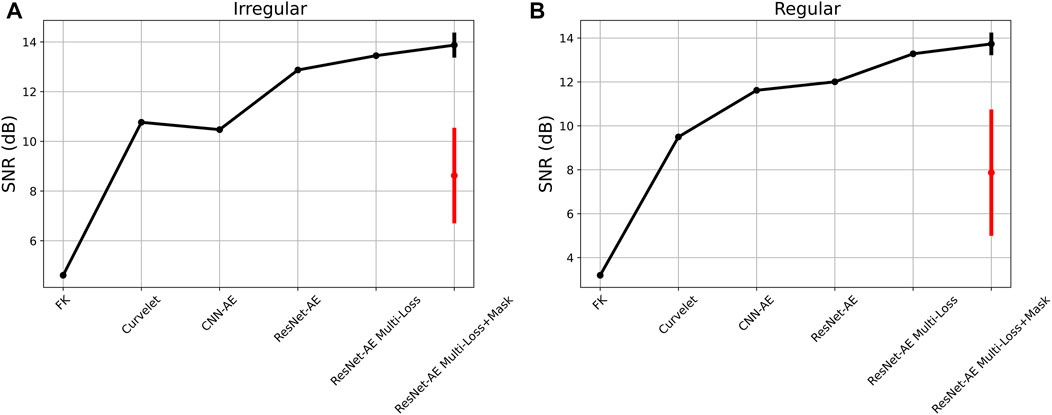
FIGURE 10. Signal-to-noise ratio as function of different inversion algorithms for the irregular (A) and regular (B) subsampling scenarios. Vertical black lines refer to the standard deviation of 5 inversion using networks with different weight initialization. Vertical red lines refer to the standard deviation of 5 inversion using the same networks and randomly initialized latent codes.
We move now onto the second synthetic dataset. The training process is performed by creating patches of size 64 × 64 in the common receiver domain using the strategy that led to the best results in the previous example. Despite the complexity of the recorded wavefield, the AE network trained with a latent code of size z = 300 is able to capture a strong representation of the seismic data, producing a decoder with strong interpolation capabilities. Figures 11, 12 display the deghosted and reconstructed upgoing wavefields by means of our AE preconditioner (Figures 11E, 12D) alongside with the subsampled data (Figures 11B, 12A), the benchmark deghosting with fully sampled data (Figures 11C, 12B), and the reconstruction by means of sparsity-promoting inversion with Curvelet transform (Figures 11D, 12C). For comparison, Figure 11A displays the fully sampled data (the first receiver ghost notch at fn1 = 15Hz ghost notch is indicated by the white arrow in the bottom panel of Figure 11A). Once again, our learned transform outperforms the best-in-class fixed-basis transform. In this example we have dropped the patched Fourier transform, since it proved to be subpar compared to the other two cases.
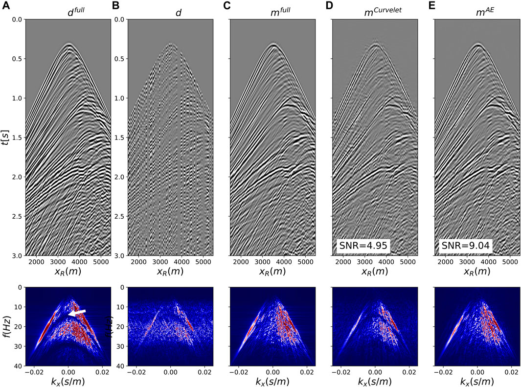
FIGURE 11. Joint deghosting and reconstruction for irregularly sampled data from the Marmousi model. (A) Full data, (B) Subsampled data, (C) Benchmark deghosted data, (D,E) Deghosted and reconstructed data using Curvelet and and AE preconditioners, respectively. All data are shown in time-space domain in the top row and frequency-wavenumber domain in the bottom row.
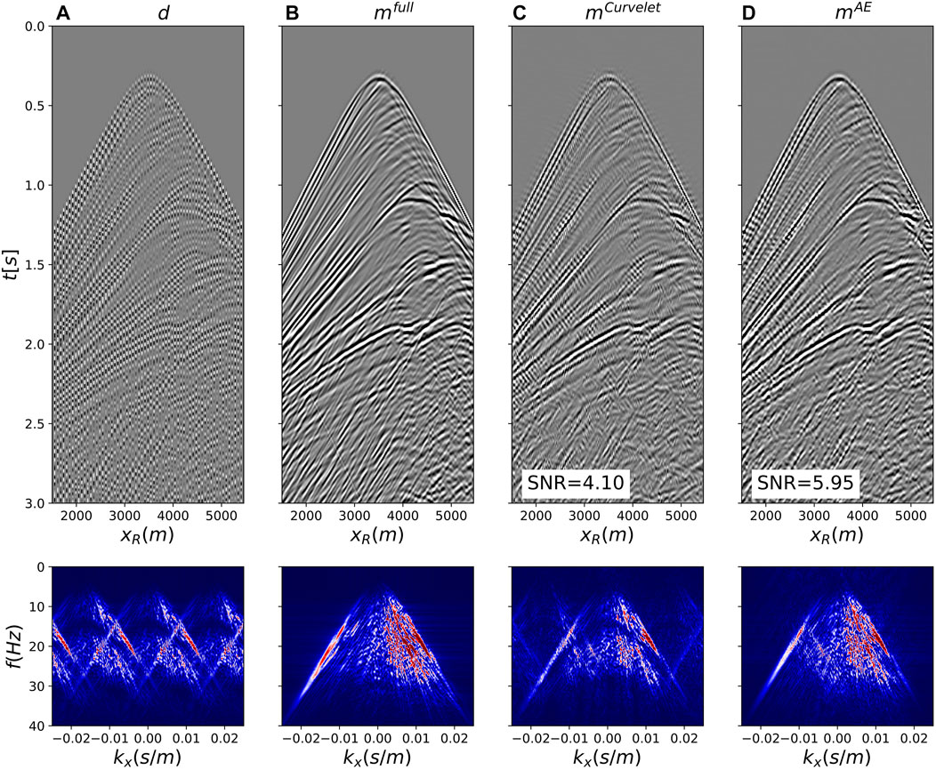
FIGURE 12. Joint deghosting and reconstruction for regularly sampled data from the Marmousi model. (A) Subsampled data, (B) Benchmark deghosted data, (C,D) Deghosted and reconstructed data using Curvelet and and AE preconditioners, respectively.
3.5 Wavefield separation and interpolation of synthetic dataset
We extend the methodology presented in the previous section to the problem of joint reconstruction and wavefield separation; this differs from the former application in that we seek to find both the up- and down-going pressure wavefields that explain the recorded multi-component seismic data. Formally, wavefield separation can be cast as an inverse problem as follows (Wapenaar, 1998; van der Neut and Herrmann, 2012):
where p and vz are the recorded pressure and vertical particle velocity data, p− and p+ are the up- and down-going separated data, I is the identity operator, and
where the latent vectors of the up- (z−) and down-going (z+) wavefields are simultaneously estimated.
The proposed approach is tested on the first synthetic dataset using multi-component receivers along the seafloor and the same two subsampling strategies (the irregularly sampled data is displayed in Figure 13A). In the training phase, the pressure recordings are sorted in the common receiver gather (CRG) and patches of size 64 × 64 are fed to the AE network with ResNet blocks and multiple losses using the same training strategies as in the deghosting example. The trained decoder is finally combined with the physical modelling operator to reconstruct the missing receivers and separate the up- and down-going components of the data: the estimated wavefields for irregular and regular subsampling are shown in Figures 13C,D, respectively. In both cases, the reconstructed wavefields closely resemble those obtained by performing a standard wavefield separation on the original, finely sampled data (Figure 13B). Once again, we observe that selecting the vectors z+ and z− by feeding a crude estimate of p+ and p− obtained via simple summation (or subtraction) of the multi-component data to the encoder leads to much better reconstruction compared to using a random or zero starting guess.
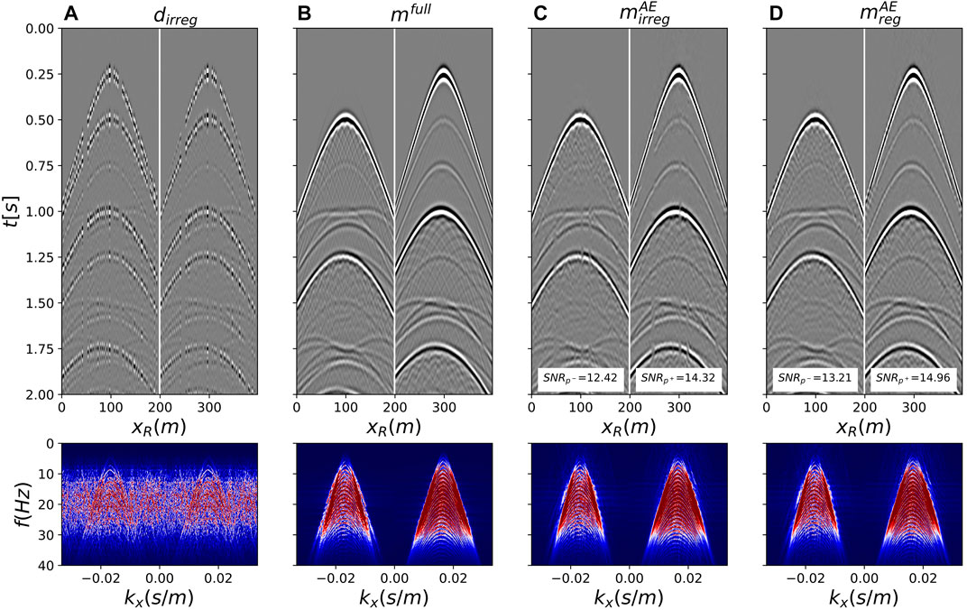
FIGURE 13. Joint wavefield separation and reconstruction for the synthetic data in ocean-bottom cable configuration. (A) Irregularly subsampled data, (B) Benchmark wavefield separated data, (C,D) Wavefield separated and reconstructed using the AE preconditioner for irregularly and regularly sampled data, respectively. All data are shown in time-space domain in the top row and frequency-wavenumber domain in the bottom row. Pressure and vertical particle velocity components are juxtaposed in panel a, whilst up- and down-going separated components are juxtaposed in all other panels.
3.6 Deghosting and interpolation of field dataset
Finally, we consider the Mobil AVO field dataset. The dataset is resorted in the common receiver domain (by extracting all pairs of traces for all sources corresponding to receivers at fixed geographical locations) and divided into approximately 52 k patches of size 64 × 64. Note that due to some irregularities in the source array, some of the patches present a small number of missing traces: no attempt is made to fill in such traces prior to training. Receivers are subsampled irregularly by retaining 60% of the original array and the training process is carried out using the network, loss, and pre-processing strategy that performed best for the synthetic examples.
After the training process is finalized, joint deghosting and interpolation is performed on a randomly selected shot gather. Figure 14 displays the original fully sampled data (panel a), the subsampled data (panel b), the benchmark deghosted wavefield (panel c), the reconstructed deghosted wavefields for the sparsity-promoting inversion with patched Fourier (panel d) and Curvelet (panel e) transforms as well as the reconstruction using the trained deep preconditioner (panel f). When compared to the benchmark solution, we can clearly observe that the inverted wavefield aided by deep preconditioners has more naturally looking seismic events and fewer artefacts than those from the fixed-basis counterparts. Moreover, the deep preconditioned inversion provides an improved reconstruction of the direct arrival (see also close-up in Figure 15): this result remarks once again the importance of learned transforms that can capture important features from the dataset at hand. Finally, note that due to the fact that receivers are towed very close to the free-surface (i.e., 10 m depth), the first receiver ghost notch is at fn1 = 75Hz. As this frequency is beyond the bandwidth of the signal, we cannot directly observe the filling of the ghost notch like in this example. However, a change in the overall amplitude balance of the spectrum of the deghosted data and the presence of sharper events in Figure 14C compared to Figure 14A are signs of a successful deghosting process.
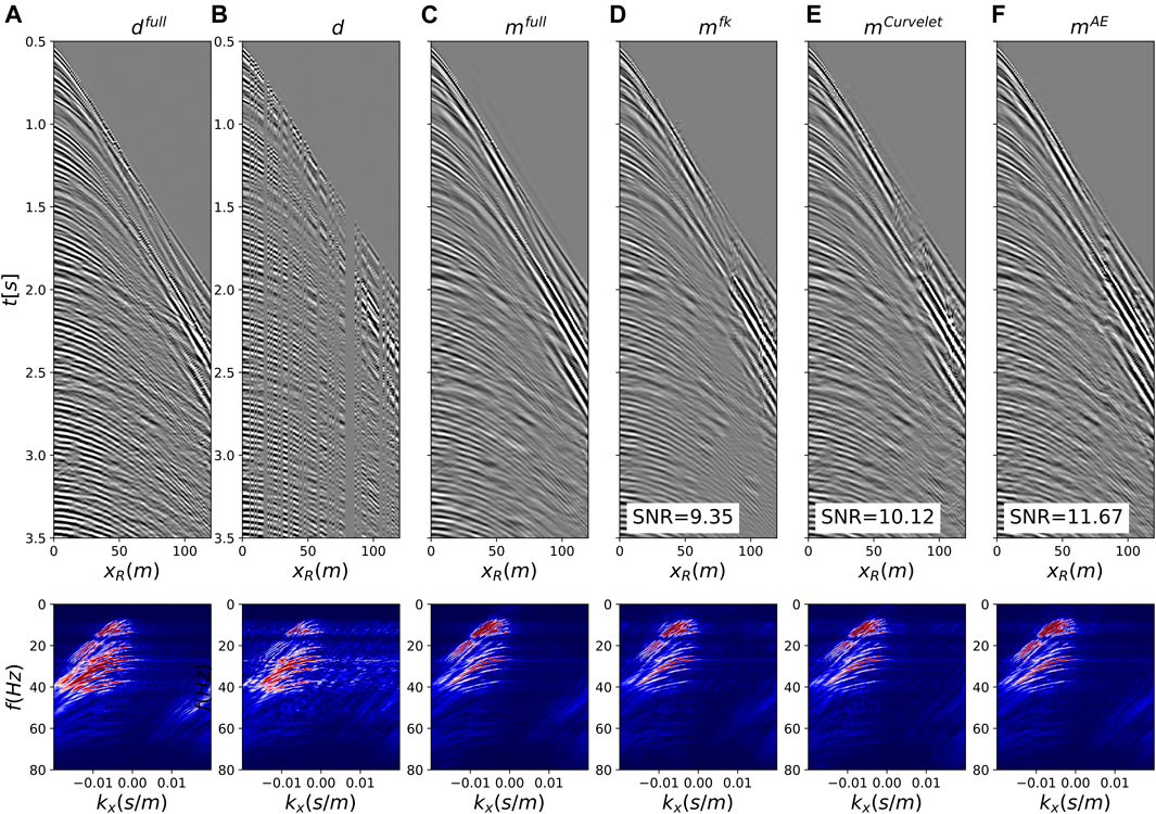
FIGURE 14. Joint deghosting and reconstruction for the field dataset with irregularly subsampled data. (A) Full data, (B) Subsampled data, (C) Benchmark deghosted data, (D–F) Deghosted and reconstructed using F-K, Curvelet, and AE preconditioners, respectively. All data are shown in time-space domain in the top row and frequency-wavenumber domain in the bottom row.
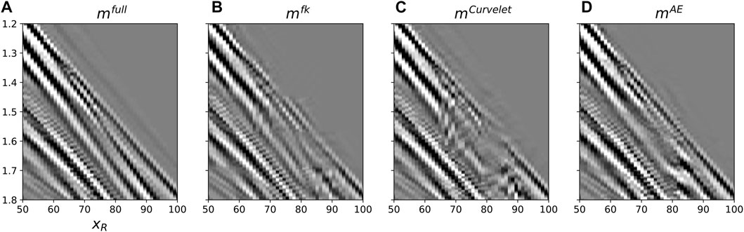
FIGURE 15. Close-ups of Figure 14 in an area around the direct arrival in the presence of a large gap. (A) Benchmark deghosted data, (B–D) Deghosted and reconstructed using F-K, Curvelet, and AE preconditioners, respectively.
4 Discussion
Deep Preconditioners represent an effective tool to regularize severely ill-posed inverse problems like those usually encountered in geophysical data processing. As shown in the Numerical examples section, by learning the characteristic features of seismic data, an AE network provides a nonlinear transformation (i.e., its decoder) that is suitable to aid the solution of seismic processing tasks such as interpolation or wavefield separation. This is further shown to outperform sparsity-promoting inversion with state-of-the-art fixed, linear bases, such as those obtained from the F-K or Curvelet transforms.
The success of the proposed approach does however rely on the availability of suitable training data and the definition of an appropriate training pipeline. Different strategies could be adopted to define the training dataset. In this work, we have shown how the dataset that we wish to process could be sorted into a domain whose seismic features are similar to those expected in the outcome of the processing step of interest. For example, when seismic data are acquired using ocean-bottom-cable acquisition systems, sources are usually well sampled in space whilst receivers are usually deployed further apart (at least in the crossline direction). By leveraging reciprocity, data sorted along receivers (i.e., common receiver domain) can be used to learn a strong representation of seismic data that are finely sampled in the spatial direction; the learned decoder can be subsequently deployed to reconstruct the missing receivers into a regular and finely sampled grid equal to that of the available sources. Note that in our synthetic example of joint interpolation and wavefield separation, despite the fact the input data used to train the AE network has not been previously decomposed into its up- and down-going constituents, the features learned from such data are shown to be representative of the output data (i.e., separated wavefields) and therefore the decoder of the network can be successfully used as preconditioner to the interpolation and decomposition process. Alternatively, a dataset acquired in a nearby field or during a previous acquisition campaign may be used as input to the AE network. In this case, the chosen dataset must have a more favourable acquisition design, i.e. sources and/or receivers are acquired over a finer spatial grid. In the field data example, to mimic such a scenario we have divided the recorded dataset into two subsets and used the first to train the AE network with the aim of recovering missing receivers in the latter subset. When dealing with streamer data, this is the only viable strategy when we wish to regularize the data along the receiver coordinate: in fact, when receivers are randomly missing or sampled along a coarse regular grid, data sorted in the common receiver domain will also be missing some traces associated with source-receiver pairs that are not sampled, due the fact that receivers move alongside with sources. On the other hand, we note that if our interest is that of recovering missing sources (whilst having access to a finely sampled receiver grid), the first strategy can be employed both for the streamer and ocean-bottom-cable scenarios. In this case, resorting the data in the common source domain provides us with regularly sampled data that can be used to train an AE network to learn useful latent representations. The trained decoder can be ultimately employed to deghost and interpolate the seismic data on the source side.
Recently, a different application of our Deep Preconditoners has been proposed by Xu et al. (2022) in the context of seismic data deblending. By leveraging the fact that blended data in the common source domain present similar features to the deblended data (i.e., coherent seismic events), the authors trained an AE network to learn a robust latent representation from such a data. The decoder is then used in the deblending process to denoise the blended data in the common receiver domain, where the blending noise appears as burst-like, trace coherent noise. Since the AE has never seen such with such kind of signal during training, the decoder is naturally encouraged to reproduce only the coherent part of the data during the deblending process. This result highlights the versatility of our approach provided that a suitable training domain can be identified from the available data. Similarly, whilst a single processing task has been carried out in all of the presented examples, another appealing property of the proposed approach lies in the fact that a single learned representation could be used for multiple subsequent tasks. For example, the same representation learned from blended common source gathers could be used to deblend and subsequently interpolate data along the source axis. If successful, this idea may provide a data-centric as opposed to task-centric approach to seismic processing with deep learning where the reliance on training is reduced to a limited number of stages in the processing chain.
Other approaches have recently emerged in the machine learning literature in the context of representation learning. Similar to the AE approach used here, all methods share the common factor of being self-supervised, i.e., do not require labels. Contrastive learning (Liu et al., 2021) is one such self-supervised learning technique that has been shown to be able to discover general features of a dataset by simply teaching a model to discriminate between similar and dissimilar training samples. In the spirit of avoiding any manual annotation, data augmentation techniques such as cropping or rotation are used to transform a single input into a number of similar inputs. The model is then fed with both similar and dissimilar pairs and trained to learn to produce latent representations that are close to each other for the first kind of pairs and far away for the other set of pairs. Future work will investigate the suitability of contrastive learning in the context of Deep Preconditioners.
Finally, whilst the proposed methodology is deterministic in that a single, best-fitting solution is obtained when solving an inverse problem with the aid of a Deep Precondioner, uncertainty quantification of neural network solutions is another active area of research in the deep learning community. Variational AutoEncoders (Kingma and Welling, 2014), a form of probabilistic autoencoding networks, represent a natural candidate to extend the proposed methodology towards multi-realization and uncertainty quantification in inverse problems. Alternatively, generative models such as Generative Adversarial Networks (GANs)—Goodfellow et al. (2014) and Normalizing Flows (Rezende and Mohamed, 2015) have also recently been used in various geophysical applications (Zhao et al., 2019; Mosser et al., 2020; Siahkoohi et al., 2022).
5 Conclusion
In this work, we have proposed a general framework to aid the solution of geophysical inverse problems by means of nonlinear, learned preconditioners. Operating in a two-steps fashion, a strong latent representation is first learned from the input seismic data in an unsupervised manner using an AutoEncoder network; the learned decoder is subsequently used to drive the solution of the physics-driven inverse problem at hand. The strength of our approach lies in the fact that no training data is required beyond the input data itself: for example, seismic data containing ghost arrivals are shown to contain useful information that can be later applied to obtained their deghosted counterpart. Different choices of network architectures, loss functions, and pre-processing have been investigated and shown to greatly impact the effectiveness of the representation learning process, and ultimately that of the downstream processing task. More specifically in our numerical examples, the combination of ResNet blocks, multiple losses with learned weights, and masked inputs resulted in deghosting (or wavefield separation) and interpolation capabilities that outperform state-of-the-art sparsity based methods with fixed, linear transformations. We also observe that the data normalization choice is crucial in ensuring a stable training process and the choice of the initialization is fundamental to achieve a stable inversion process. Moreover, our numerical examples suggest that the proposed method can be equally used in the presence of irregularly or regularly subsampled data. This greatly differs from the case when conventional linear transformations are used to precondition the inverse problem; in this scenario, different strategies must be adopted based on the subsampling pattern. Finally, the proposed framework may have far wider applicability than the examples of joint reconstruction and wavefield decomposition discussed in this work; other seismic processing steps such as elastic wavefield separation, up/down deconvolution, and target-oriented redatuming will be subject of future studies.
Data availability statement
The raw data supporting the conclusion of this article will be made available by the authors, without undue reservation. The associated codes used to run the numerical examples can be accessed at https://github.com/DIG-Kaust/DeepPrecs.
Author contributions
MR contributed to conception, methodology, numerical implementation, and writing.
Acknowledgments
I thank KAUST for supporting this research. I am also grateful to Claire Birnie (KAUST) for insightful discussions. All numerical examples have been created using the PyLops (Ravasi and Vasconcelos, 2020) and PyTorch (Paszke et al., 2017) computational frameworks.
Conflict of interest
The author declares that the research was conducted in the absence of any commercial or financial relationships that could be construed as a potential conflict of interest.
Publisher’s note
All claims expressed in this article are solely those of the authors and do not necessarily represent those of their affiliated organizations, or those of the publisher, the editors and the reviewers. Any product that may be evaluated in this article, or claim that may be made by its manufacturer, is not guaranteed or endorsed by the publisher.
Footnotes
1See https://wiki.seg.org/wiki/Mobil_AVO_viking_graben_line_12 for details.
References
Abma, R., and Kabir, N. (2006). 3d interpolation of irregular data with a pocs algorithm. Geophysics 71, E91–E97. doi:10.1190/1.2356088
Adler, J., and Oktem, O. (2017). Solving ill-posed inverse problems using iterative deep neural networks. Inverse Probl. 33, 124007. doi:10.1088/1361-6420/aa9581
Alfarraj, M., and AlRegib, G. (2019). “Semi-supervised learning for acoustic impedance inversion,” SEG Technical Program Expanded Abstracts, 89th Annual International Meeting, 2298–2302. doi:10.1190/segam2019-3215902.1
Alkhalifah, T., Wang, H., and Ovcharenko, O. (2021). Mlreal: Bridging the gap between training on synthetic data and real data applications in machine learning. arXiv [Preprint]. doi:10.48550/arXiv.2109.05294
Beck, A., and Teboulle, M. (2009). A fast iterative shrinkage-thresholding algorithm for linear inverse problems. SIAM J. Imaging Sci. 2, 183–202. doi:10.1137/080716542
Bergmann, P., Lowe, S., Fauser, M., Sattlegger, D., and Steger, C. (2018). Improving unsupervised defect segmentation by applying structural similarity to autoencoders. arXiv [Preprint]. doi:10.48550/arXiv.1807.02011
Birnie, C., and Alkhalifah, T. (2022). Leveraging domain adaptation for efficient seismic denoising. Energy Data Conf. doi:10.7462/eid2022-04.1
Brougois, A., Bourget, M., Lailly, P., Poulet, M., Ricarte, P., and Versteeg, R. (1990). “Marmousi, model and data,” in European Association of Geoscientists & Engineers, Conference Proceedings, EAEG Workshop - Practical Aspects of Seismic Data Inversion.
Candès, E. J., Romberg, J., and Tao, T. (2006). Robust uncertainty principles: Exact signal reconstruction from highly incomplete frequency information. IEEE Trans. Inf. Theory 52, 489–509. doi:10.1109/tit.2005.862083
Das, V., Pollack, A., Wollner, U., and Mukerji, T. (2019). Convolutional neural network for seismic impedance inversion. Geophysics 84, R869–R880. doi:10.1190/geo2018-0838.1
Devlin, J., Chang, M.-W., Lee, K., and Toutanova, K. (2018). Bert: Pre-training of deep bidirectional transformers for language understanding. arXiv [Preprint]. doi:10.48550/arXiv.1810.04805
Fomel, S., and Liu, Y. (2010). Seislet transform and seislet frame. Geophysics 75, V25–V38. doi:10.1190/1.3380591
Fomel, S., Sava, P., Vlad, I., Liu, Y., and Bashkardin, V. (2013). Madagascar: Open-source software project for multidimensional data analysis and reproducible computational experiments. J. Open Res. Softw 1 (1), e8. doi:10.5334/jors.ag
Fomel, S. (2003). Seismic reflection data interpolation with differential offset and shot continuation. Geophysics 68, 733–744. doi:10.1190/1.1567243
Goodfellow, I., Pouget-Abadie, J., Mirza, M., Xu, B., Warde-Farley, D., Ozair, S., et al. (2014). “Generative adversarial nets,” in Advances in neural information processing.
Hauser, S., and Ma, J. W. (2012). Seismic data reconstruction via shearlet-regularized directional inpainting. Preprint.
He, K., Zhang, X., Ren, S., and Sun, J. (2015). Deep residual learning for image recognition. arXiv [Preprint]. doi:10.48550/arXiv.1512.03385
He, K., Chen, X., Xie, S., Li, Y., Dollar, P., and Girshick, R. (2021). Masked autoencoders are scalable vision learners. arXiv [Preprint]. doi:10.48550/arXiv.2111.06377
Hennenfent, G., and Herrmann, F. J. (2008). Simply denoise: Wavefield reconstruction via jittered undersampling. Geophysics 73, V19–V28. doi:10.1190/1.2841038
Herrmann, F. J., and Hennenfent, G. (2008). Non-parametric seismic data recovery with curvelet frames. Geophys. J. Int. 173, 233–248. doi:10.1111/j.1365-246x.2007.03698.x
Hotelling, H. (1933). Analysis of a complex of statistical variables into principal components. J. Educ. Psychol. 33, 417–441. doi:10.1037/h0071325
Isola, P., Zhu, J., Zhou, T., and Efros, A. (2017). “Image-to-image translation with conditional adversarial networks,” in IEEE Conference on Computer Vision and Pattern Recognition (CVPR), 5967.
Kabir, M. M. N., and Verschuur, D. J. (1995). Restoration of missing offsets by parabolic Radon transform1. Geophys. Prospect. 43, 347–368. doi:10.1111/j.1365-2478.1995.tb00257.x
Kazei, V., Ovcharenko, O., Plotnitskii, P., Peter, D., Zhang, X., and Alkhalifah, T. (2021). Mapping full seismic waveforms to vertical velocity profiles by deep learning. Geophysics 86, R711–R721. doi:10.1190/geo2019-0473.1
Kendall, A., Gal, Y., and Cipolla, R. (2018). “Multi-task learning using uncertainty to weigh losses for scene geometry and semantics,” in 2018 IEEE/CVF Conference on Computer Vision and Pattern Recognition, 7482.
Kingma, D., and Ba, J. (2014). Adam: A method for stochastic optimization. arXiv [Preprint]. doi:10.48550/arXiv.1412.6980
Kingma, D. P., and Welling, M. (2014). Auto-encoding variational bayes. arXiv [Preprint]. doi:10.48550/arXiv.1312.6114
Kong, F., Picetti, F., Lipari, V., Bestagini, P., Tang, X., and Tubaro, S. (2020). Deep prior based unsupervised reconstruction of irregularly sampled seismic data. IEEE Geosci. Remote Sens. Lett. 19, 1–5. doi:10.1109/lgrs.2020.3044455
Kramer, M. A. (1991). Nonlinear principal component analysis using autoassociative neural networks. AIChE J. 37, 233–243. doi:10.1002/aic.690370209
Kuijpers, D., Vasconcelos, I., and Putzky, P. (2021). Reconstructing missing seismic data using deep learning. arXiv [Preprint]. doi:10.48550/arXiv.2101.09554
Kumar, R., Aravkin, A., and Herrmann, F. (2012). “Fast methods for rank minimization with applications to seismic-data interpolation,” in SEG Technical Program Expanded Abstracts, 82nd Annual International Meeting.
Li, H., Schwab, J., Antholzer, S., and Haltmeier, M. (2020). Nett: Solving inverse problems with deep neural networks. Inverse Probl. 36, 065005. doi:10.1088/1361-6420/ab6d57
Liu, Y., and Fomel, S. (2011). Seismic data interpolation beyond aliasing using regularized nonstationary autoregression. Geophysics 76, V69–V77. doi:10.1190/geo2010-0231.1
Liu, X., Zhang, F., Hou, Z., Mian, L., Wang, Z., Zhang, J., et al. (2021). Self-supervised learning:generative or contrastive. IEEE Trans. Knowl. Data Eng., 1. doi:10.1109/tkde.2021.3090866
Lønning, K., Putzky, P., Sonke, J.-J., Reneman, L., Caan, M., and Welling, M. (2019). Recurrent inference machines for reconstructing heterogeneous mri data. Med. Image Anal. 53, 64–78. doi:10.1016/j.media.2019.01.005
Luiken, N., Ravasi, M., and Birnie, C. (2022). A hybrid approach to seismic deblending: When physics meets self-supervision. arXiv [Preprint]. doi:10.48550/arXiv.2205.15395
Mandelli, S., Lipari, V., Bestagini, P., and Tubaro, S. (2019). Interpolation and denoising of seismic data using convolutional neural networks. arXiv [Preprint]. doi:10.48550/arXiv.1901.07927
Masci, J., Meier, U., Ciresan, D., and Schmidhuber, J. (2011). “Stacked convolutional auto-encoders for hierarchical feature extraction,” in ICANN 2011: Artificial Neural Networks and Machine Learning.
Morningstar, W., Levasseur, L., Hezaveh, Y., Blandford, R., Marshall, P., Putzky, P., et al. (2019). Data-driven reconstruction of gravitationally lensed galaxies using recurrent inference machines. Astrophys. J. 14. doi:10.3847/1538-4357/ab35d7
Mosser, L., Dubrule, O., and Blunt, M. (2020). Stochastic seismic waveform inversion using generative adversarial networks as a geological prior. Math. Geosci. 52, 53–79. doi:10.1007/s11004-019-09832-6
Nocedal, J. (1980). Updating quasi-Newton matrices with limited storage. Math. Comput. 35, 773–782. doi:10.1090/s0025-5718-1980-0572855-7
Obmann, D., Nguyen, L., Schwab, J., and Haltmeier, M. (2020). Sparse anett for solving inverse problems with deep learning. arXiv [Preprint]. doi:10.48550/arXiv.2004.09565
Oropeza, V., and Sacchi, M. (2011). Simultaneous seismic data denoising and reconstruction via multichannel singular spectrum analysis. Geophysics 76, V25–V32. doi:10.1190/1.3552706
Ovcharenko, O. (2021). Data-driven methods for the initialization of full-waveform inversion. PhD Thesis. King Abdullah University of Science and Technology. doi:10.25781/KAUST-ERWD3
Ozbek, A., Vassallo, M., Ozdemir, K., van Manen, D., and Eggenberger, K. (2010). Crossline wavefield reconstruction from multicomponent streamer data: Part 2 — Joint interpolation and 3d up/down separation by generalized matching pursuit. Geophysics 75, WB69–WB85. doi:10.1190/1.3497316
Park, J., Jennings, J., Clapp, B., and Biondi, B. (2020). Seismic data interpolation using a pocs-guided deep image prior. SEG Technical Program Expanded Abstracts. doi:10.1190/segam2020-3427320.1
Paszke, A., Gross, S., Chintala, S., Chanan, G., Yang, E., DeVito, Z., et al. (2017). “Automatic differentiation in pytorch,” in NIPS-W.
Picetti, F., Lipari, V., Bestagini, P., and Tubaro, S. (2021). “Anti-aliasing add-on for deep prior seismic data interpolation,” in IEEE International Conference on Image Processing (ICIP).
Picetti, F. (2022). A study on deep learning methodologies applied to geophysical inverse problems. Ph. D. Thesis. Politecnico di Milano.
Ravasi, M., and Vasconcelos, I. (2020). PyLops—a linear-operator Python library for scalable algebra and optimization. SoftwareX 11, 100361. doi:10.1016/j.softx.2019.100361
Ravasi, M. (2021). Seismic wavefield processing with deep preconditioners. SEG/AAPG/SEPM First International Meeting for Applied Geoscience & Energy. doi:10.1190/segam2021-3580609.1
Rezende, D., and Mohamed, S. (2015). “Variational inference with normalizing flows,” in International Conference on Machine Learning.
Richardson, A., and Feller, C. (2019). Seismic data denoising and deblending using deep learning. arXiv [Preprint]. doi:10.48550/arXiv.1907.01497
Roweis, S., and Hinton, G. (2002). “Stochastic neighbor embedding,” in Neural Information Processing Systems.
Ruan, J., and Vasconcelos, I. (2019). Data- and prior-driven sampling and wavefield reconstruction for sparse, irregularly-sampled, higher-order gradient data. SEG Technical Program Expanded Abstracts, 4515–4519. doi:10.1190/segam2019-3216425.1
Saad, O. M., and Chen, Y. (2020). Deep denoising autoencoder for seismic random noise attenuation. Geophysics 85, V367–V376. doi:10.1190/geo2019-0468.1
Sacchi, M., and Ulrych, T. (1995). High-resolution velocity gathers and offset space reconstruction. Geophysics 60, 1169–1177. doi:10.1190/1.1443845
Schonewille, M., Klaedtke, A., and Vigner, A. (2009). “Anti-alias anti-leakage Fourier transform,” SEG Technical Program Expanded Abstracts, 79th Annual International Meeting, 3249–3253. doi:10.1190/1.3255533
Shi, Y., Wu, X., and Fomel, S. (2019). Saltseg: Automatic 3d salt segmentation using a deep convolutional neural network. Interpretation 7, SE113–SE122. doi:10.1190/int-2018-0235.1
Siahkoohi, A., Kumar, R., and Herrmann, F. (2018). Seismic data reconstruction with generative adversarial networks. 80th EAGE Conf. Exhib. doi:10.3997/2214-4609.201801393
Siahkoohi, A., Rizzuti, G., Orozco, R., and Herrmann, F. J. (2022). Reliable amortized variational inference with physics-based latent distribution correction. arXiv [Preprint]. doi:10.48550/arXiv.2207.11640
Smith, L. N., and Topin, N. (2017). Super-convergence: Very fast training of neural networks using large learning rates. arXiv [Preprint]. doi:10.48550/arXiv.1708.07120
Spitz, S. (1991). Seismic trace interpolation in the f-x domain. Geophysics 56, 785–794. doi:10.1190/1.1443096
Sun, J., Slang, S., Elboth, T., Greiner, T. L., McDonald, S., and Gelius, L.-J. (2020). A convolutional neural network approach to deblending seismic data. Geophysics 85, WA13–WA26. doi:10.1190/geo2019-0173.1
Trad, D., Ulrych, T., and Sacchi, M. (2002). Accurate interpolation with high-resolution time-variant radon transforms. Geophysics 67, 644–656. doi:10.1190/1.1468626
Trickett, S., Burroughs, L., Milton, A., Walton, L., and Dack, R. (2010). Rank-reduction-based trace interpolation. SEG Technical Program Expanded Abstracts, 80th Annual International Meeting, 3829–3833. doi:10.1190/1.3513645
Ulyanov, D., Vedaldi, A., and Lempitsky, V. (2017). Deep image prior. arXiv [Preprint]. doi:10.48550/arXiv.1711.10925
van der Neut, J., and Herrmann, F. J. (2012). “Reciprocity properties of one-way propagators,” in 74th EAGE Conference and Exhibition, European Association of Geoscientists & Engineers.
Vasconcelos, I., Peng, H., Ravasi, M., and Kuijpers, D. (2022). “Deep learning in seismic inverse problems with recurrent inference machines,” in 83rd EAGE Annual Conference & Exhibition Workshop.
Vassallo, M., Ozbek, A., Ozdemir, K., and Eggenberger, K. (2010). Crossline wavefield reconstruction from multicomponent streamer data: Part 1 — Multichannel interpolation by matching pursuit (mimap) using pressure and its crossline gradient. Geophysics 75, WB53–WB67. doi:10.1190/1.3496958
Vincent, P. (2008). “Extracting and composing robust features with denoising autoencoders,” in ICML ‘08: Proceedings of the 25th international conference on machine learning, 1096–1103. doi:10.1145/1390156.1390294
Waldeland, A. U., Jensen, A. C., Gelius, L.-J., and Schistad Solberg, A. H. (2018). Convolutional neural networks for automated seismic interpretation. Lead. Edge 37, 529–537. doi:10.1190/tle37070529.1
Wapenaar, K. (1998). Reciprocity properties of one-way propagators. Geophysics 36, 1795–1798. doi:10.1190/1.1444473
Wu, X., Liang, L., Shi, Y., and Fomel, S. (2020). Faultseg3d: Using synthetic data sets to train an end-to-end convolutional neural network for 3d seismic fault segmentation. Geophysics 84, IM35–IM45. doi:10.1190/geo2018-0646.1
Xu, W., Lipari, V., Bestagini, P., Ravasi, M., Chen, W., and Tubaro, S. (2022). Intelligent seismic deblending through deep preconditioner. IEEE Geosci. Remote Sens. Lett. 19, 1–5. doi:10.1109/lgrs.2022.3193716
Yang, F., and Ma, J. (2019). Deep-learning inversion: A next-generation seismic velocity model building method. Geophysics 84, R583–R599. doi:10.1190/geo2018-0249.1
Yang, Y., Ma, J., and Osher, S. (2013). Seismic data reconstruction via matrix completion. Inverse Probl. ImagingSpringf. 7, 1379–1392. doi:10.3934/ipi.2013.7.1379
Yu, S., and Ma, J. (2021). Deep learning for geophysics: Current and future trends. Rev. Geophys. 59. doi:10.1029/2021rg000742
Yu, S., Ma, J., and Wang, W. (2021). Deep learning for denoising. Geophysics 84, V333–V350. doi:10.1190/geo2018-0668.1
Zhao, X., Curtis, A., and Zhang, X. (2019). Bayesian seismic tomography using normalizing flows. Geophys. J. Int. 228, 213–239. doi:10.1093/gji/ggab298
Zhao, T. (2018). “Seismic facies classification using different deep convolutional neural networks,” in SEG Technical Program Expanded Abstracts, 88th Annual International Meeting.
Keywords: seismic processing, seismic data analysis, dimensionality reduction, unsupervised learning, deep learning, inverse problems, regularization, geophysics
Citation: Ravasi M (2022) Deep preconditioners and their application to seismic wavefield processing. Front. Earth Sci. 10:997788. doi: 10.3389/feart.2022.997788
Received: 19 July 2022; Accepted: 29 August 2022;
Published: 26 September 2022.
Edited by:
Yasir Bashir, Universiti Sains Malaysia (USM), MalaysiaReviewed by:
Dario Grana, University of Wyoming, United StatesYibo Wang, Institute of Geology and Geophysics (CAS), China
Amin Roshandel Kahoo, Shahrood University of Technology, Iran
Keyvan Khayer, Shahrood University of Technology, Iran
Copyright © 2022 Ravasi. This is an open-access article distributed under the terms of the Creative Commons Attribution License (CC BY). The use, distribution or reproduction in other forums is permitted, provided the original author(s) and the copyright owner(s) are credited and that the original publication in this journal is cited, in accordance with accepted academic practice. No use, distribution or reproduction is permitted which does not comply with these terms.
*Correspondence: Matteo Ravasi, bWF0dGVvLnJhdmFzaUBrYXVzdC5lZHUuc2E=