Design a regional and multistep air quality forecast model based on deep learning and domain knowledge

Air pollution is an issue across the world. It not only directly affects the environment and human health, but also influences the regional and even global climate by changing the atmospheric radiation budget, resulting in extensive and serious adverse effects. It is of great significance to accurately predict the concentration of pollutant. In this study, the domain knowledge of Atmospheric Sciences, advanced deep learning methods and big data are skillfully combined to establish a novel integrated model TSTM, derived from its fundamental features of Time, Space, Type and Meteorology, to achieve regional and multistep air quality forecast. Firstly, Expectation Maximization and Min-Max algorithms are used for the interpolation and normalization of data. Secondly, feature selection and construction are accomplished based on domain knowledge and correlation coefficient, and then Sliding Time Window algorithm is employed to build the supervised learning task. Thirdly, the features of pollution source and meteorological condition are learned and predicted by CNN-BiLSTM-Attention model, the integrated model of convolutional neural network and Bidirectional long short-term memory network based on Sequence to Sequence framework with Attention mechanism, and then Convolutional Long Short-Term Memory Neural Network (ConvLSTM) integrates the two determinant features to obtain predicted pollutant concentration. The multiple-output strategy is also employed for the multistep prediction. Lastly, the forecast performance of TSTM for pollutant concentration, air quality and heavy pollution weather is tested systematically. Experiments are conducted in Beijing-Tianjin-Hebei Air Pollution Transmission Channel (“2+26” cities) of China for multistep prediction of hourly concentration of six conventional air pollutants. The results show that the performance of TSTM is better than other benchmark models especially for heavy pollution weather and it has good robustness and generalization ability.

1 Introduction

With the rapid development of industrialization and urbanization, more and more fossil fuels are burned, resulting in the deterioration of air quality and frequent haze weather (Jerrett, 2015; Mo et al., 2021; Mu et al., 2021). As a serious environmental problem air pollution has attracted worldwide attention. Air pollution is the single greatest environmental risk to human health and one of the main avoidable causes of death and disease globally, with some estimated 6.5 million premature deaths (2016) across the world attributed to indoor and outdoor air pollution (United Nations Environment Programme, 2022). Predicting air pollution in advance is of great significance to the health guide of the public and the pollution control of government (Li et al., 2019).

Numerical forecast and statistical forecast are mainstream methods for air quality forecast. The numerical forecast model predicts the concentration of air pollutants by simulating the transmission and diffusion of pollutants in the atmosphere. Numerical forecast has more advantages in regional pollution forecast and analysis, but it has higher demands on input data and computation power. Commonly used models are based on the Weather Research and Forecasting Model (WRF). Spiridonov et al. (Spiridonov et al., 2019) configured and designed an air quality system based on the WRF coupled with chemistry (WRF-Chem) for Macedonia. A generalized additive model was also developed to predict the concentration of PM_2.5 by using the WRF to obtain the input of the prediction model (Sahu et al., 2020). And Cheng et al. (Cheng et al., 2021) proposed an air quality forecasting system composed of WRF and Community Multiscale Air Quality Modeling System (CMAQ) and a bias-correction method to improve the accuracy of forecast. The statistical forecast model obtains predicted pollutant concentration in the basis of statistical analysis on historical data of pollutant and meteorology. Statistical forecast is relatively more efficient and practical, while it has limitations for the prediction of hourly concentration and heavy pollution. Common statistical models are multiple linear regression model (MLR) and autoregressive integrated moving average model (ARIMA). Ng et al. established a MLR based on meteorological factors and air pollutants to predict the daily average concentration of PM₁₀, and obtained good prediction performance (Ng and Awang, 2018). Pohoata et al. used the ARIMA to predict pollutants, and the results showed that the prediction performance of PM and CO was poor, but the prediction of NO_X and O₃ achieved relatively good results (Pohoata and Lungu, 2017).

In recent years artificial intelligence (AI) has acquired the rapid development, especially machine learning has been applied in various fields and great success was achieved. Machine learning technologies effectively serve air pollution forecast too, and there are relatively more applications of traditional machine learning algorithms. Perisic et al. (Perišić et al., 2017) used the boosted decision tree model to predict the hourly concentration of PM₁₀ at different stations, and found that the prediction performance of the model at different stations was affected by emission sources, topography and local climate. Chen (Chen, 2018) applied Back Propagation Neural Network combined with PM_2.5 concentration, temperature, humidity, wind force and satellite remote sensing data of aerosol optical thickness, and realized the high-precision prediction of PM_2.5 in the next 3 hours. Cheng et al. (Cheng et al., 2019) combined Empirical Mode Decomposition (EMD) with Support Vector Regression (SVR) to forecast daily air quality index (AQI) of Xingtai in China. Li et al. (Li et al., 2020) designed a geographically and temporally weighted generalized regression neural network (GTW-GRNN) to estimate ground NO₂ concentrations by integrating ground NO₂ station measurements. Mo et al. (Mo et al., 2019) combined Improved Complete Ensemble Empirical Mode Decomposition with Adaptive Noise (ICEEMDAN), Whale Optimization Algorithm (WOA) and Extreme Learning Machine (ELM) to design prediction model and acquired superior effect in daily concentration prediction of conventional air pollutants. The applications of deep learning to air quality forecast attract increasingly more attention. Chakma et al. (Chakma et al., 2017) collected street view photos containing sky, buildings and pollution category labels in Beijing from 2013 to 2017 to train convolutional neural network (CNN), and the accuracy of the model in predicting air pollution category through photos can reach 68.74%. Kim et al. (Kim et al., 2018) compared the performance of traditional machine learning model multilayer perceptron, deep learning model Elman neural network and long-short term memory network (LSTM) in predicting ozone concentration, and the experiment shows that the performance of LSTM is better and the error growth rate of LSTM is smaller with the increase of prediction time. Pak et al. (Pak et al., 2020) combined CNN, LSTM and the historical data of air quality and meteorological elements related to the target based on mutual information (MI), and realized the one-step prediction of the daily average concentration of PM_2.5 in Beijing. Convolutional Long Short-Term Memory Neural Network (ConvLSTM) was used by Wen et al. (Wen et al., 2019) to predict hourly PM_2.5 concentration of all monitoring stations in China. Wang et al. (Wang et al., 2020) predicted hourly ozone concentration of 35 monitoring stations in Beijing by Sequence to Sequence model (Seq2Seq). In addition, other forecast methods based on AI have also been proposed in recent years (Zhao et al., 2019; Mo et al., 2020; Ulpiani et al., 2022; Yu et al., 2022).

However, there are still shortages in previous studies, and air quality forecast based on AI needs to be further improved. Previous studies always focus on single pollutant, but actually six conventional air pollutants PM_2.5, PM₁₀, CO, NO₂, SO₂, O₃ are essential for air quality prediction and early warning. For example, AQI must rely on predicted concentrations of the six pollutants to report future air quality level and chief pollutant. This deficiency also leads to an incomplete evaluation of model performance. Missing data is a common problem and can cause serious impacts to data-driven model, but it is usually neglected. Besides data, algorithm and computing power, domain knowledge plays a critical role in the application of AI algorithm, but the modeling of air quality forecast always ignores this point. Furthermore, the application of deep learning to air quality forecast is an important research direction, and it is urgent to conduct numerous studies to comprehensively explore the applicability of deep learning algorithms to air pollution prediction and develop appropriate models¹.

To overcome shortcomings of previous studies, we introduce the domain knowledge of Atmospheric Sciences to design a novel integrated model based on deep learning to perform regional and multistep forecast of six air pollutants in this study. Our model is called TSTM because of its four key features including Time, Space, Type and Meteorology. It is worth mentioning that TSTM is the result of combining the theories of Atmospheric Sciences and deep learning technologies. First of all, the theories of Atmospheric Sciences help grasp the evolution mechanism of air pollution and determinants of pollutant concentration, and then the forecast framework are also designed based on related domain knowledge. Secondly, it is needed to find solutions from deep learning models to dispose important factors for prediction. It can be seen from previous studies that CNN and LSTM are preferred in air pollution prediction because of their superiority in feature extraction and learning long and short-term correlations in big data (Ian et al., 2017). Therefore, CNN and advanced versions of LSTM, namely Bidirectional long short-term memory network (BiLSTM) and ConvLSTM, are applied. Moreover, Seq2Seq framework is used to establish integrated model, and Attention mechanism is helpful to multiple-feature task. At last, a comprehensive evaluation plan is proposed from the perspective of Atmospheric Sciences too. Besides common statistical indicators, more practical evaluation is conducted involving air quality level, chief pollutant, heavy pollution weather and so on, which is the focus of the public and government.

The workflow of TSTM can be summarized as follows. Firstly, Expectation Maximization algorithm (EM) efficiently deals with missing data and Min-Max normalization can improve the convergence speed and accuracy of model. Secondly, domain knowledge of Atmospheric Sciences helps us decide preliminary features and effective features are further selected by correlation coefficient, and then feature decomposition and combination as well as the sliding time window algorithm is applied to transform the original time series into the supervised learning task. Thirdly, CNN-BiLSTM-Attention, an integrated model of CNN and BiLSTM by Seq2Seq with Attention mechanism, is used to learn and forecast pollution source and meteorological condition features separately, and then ConvLSTM couples them to obtain predicted pollutant concentration. Furthermore, multiple-output strategy is employed for multi-step prediction, which achieves high efficiency and low cost. Finally, a comprehensive performance evaluation scheme is designed referencing “Technical guideline for numerical forecasting of ambient air quality (HJ 1130-2020)” issued by China’s Ministry of Ecology and Environment (The Ministry of Ecology and Environment of China, 2022a). Evaluation involves three aspects, namely, pollutant concentration forecast, air quality forecast and heavy pollution weather forecast. TSTM is tested on two independent test sets for the multi-step prediction of the hourly concentration of six conventional air pollutants in Beijing-Tianjin-Hebei Air Pollution Transmission Channel (“2+26” cities) of China.

2 Data and methods

2.1 Study area

Recently regional and compound air pollution is increasingly notable. Beijing-Tianjin-Hebei and surrounding regions belong to the core economic zone of China but the most polluted region with prominent cross-region air pollution, which has caused serious concern from the public and government. The Ministry of Ecology and Environment of China determined Beijing-Tianjin-Hebei Air Pollution Transmission Channel (“2+26” cities) involving 6 provinces in 2017 and established its special emission limits of air pollutants in 2018. Therefore, Beijing-Tianjin-Hebei Air Pollution Transmission Channel (“2+26” cities) as Figure 1 shows is chosen as study area for its important strategic position and space correlation of air pollution.

FIGURE 1

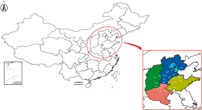
FIGURE 1. The Beijing-Tianjin-Hebei Air Pollution Transmission Channel (“2+26” cities).

2.2 Data

Six conventional air pollutants (PM_2.5, PM₁₀, CO, NO₂, SO₂, O₃) are necessary items for air quality forecast and evaluation, especially AQI must rely all of them. As to meteorological elements, we collect data of wind speed, temperature, relative humidity and precipitation based on the domain knowledge of Atmospheric Science. Hourly monitoring data of 6 air pollutants and 4 meteorological elements during 2017.12–2019.2 of 28 cities are collected from The Ministry of Ecology and Environment of China² and China Meteorological Administration³. Same architecture of forecast model is shared, while the model for each pollutant in each city needs to be trained and evaluated separately. The total number of data participating in modeling is approximately 100 million, which means actually big data. Data from 2017.12 to 2018.12 are used as training set, and the data of 2019.1 are used as validation set while the data of 2019.2 are selected as test set. The hyperparameters are tuned manually and determined based on the performance of model on validation set. In addition, in order to test the generalization ability of the model, the data of 2019.6 are supplemented as an additional test set.

2.3 Methods

2.3.1 Convolutional neural network

Convolutional neural network (CNN) is a feedforward neural network with convolution operation and depth structure (Lecun, 1989). It is a classical deep learning algorithm. The research on CNN began in the 1980s. After the 21st century, with the proposal of deep learning theory and the improvement of numerical computing ability, it has developed rapidly. Based on the visual perception of biology, it has been successfully used in computer vision, natural language processing and so on because of its sparse connection and weight sharing. CNN is usually composed of input layer, convolutional layer, pooling layer, fully-connected layer and output layer (Figure 2).

FIGURE 2

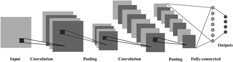
FIGURE 2. The architecture of CNN.

2.3.2 Long short-term memory network

Long Short-Term Memory Network (LSTM) (Hochreiter and Schmidhuber, 1997) is an improved model of Recurrent Neural Network (RNN). It replaces hidden node with memory block to solve the problem of gradient disappearance or explosion after many time steps. Memory block is made up of memory cell, forget gate, input gate and output gate. Figure 3 presents the architecture of LSTM. LSTM is skilled in learning from experience and processing time series with unknown time delay between important events. It has been successfully applied to handwritten character recognition, machine translation and so forth.

FIGURE 3

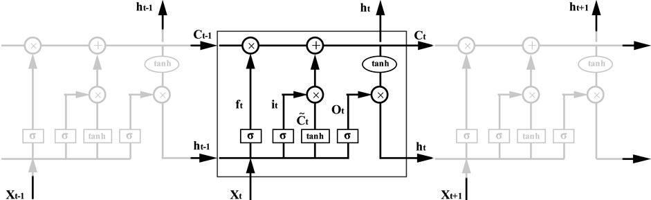
FIGURE 3. The architecture of LSTM.

2.3.3 Bidirectional long short-term memory network

The traditional recurrent neural network can only predict the output of the current time according to the historical information. However, in some cases, the output of the current moment is closely related to the history and future state, so considering the context information at the same time is conducive to comprehensive judgment. Bidirectional long short-term memory network (BiLSTM) solves this problem. It consists of two unidirectional LSTM (Schuster and Paliwal, 1997) (Figure 4). The input at each time will be provided to the forward and backward LSTM at the same time. The two hidden layers calculate the state and output independently. The final output of the BiLSTM is jointly determined by the outputs of the two LSTM.

FIGURE 4

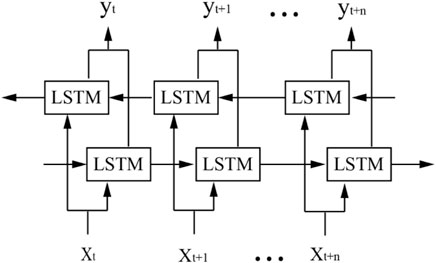
FIGURE 4. The architecture of BiLSTM.

2.3.4 Convolutional long short-term memory network

Convolutional long short-term memory network (ConvLSTM) is a variant of LSTM (Shi et al., 2015). The conventional LSTM belongs to the fully connected LSTM (FC-LSTM), that is, the input to state and state to state connections are calculated by feedforward neural network. ConvLSTM replaces this connection with convolution, which not only has the time series processing advantage of LSTM, but also obtains the feature extraction ability of CNN.

2.3.5 Sequence to sequence

Sequence to Sequence (Seq2Seq) is a variant of RNN, and Encoder and Decoder are its main parts. This framework is proposed for the case that the length of input sequence and output sequence is unequal. Two neural networks are treated as Encoder and Decoder respectively, and Encoder reads and compresses input sequence to a vector C with fixed length which is then read and processed by Decoder according to target sequence (Cho et al., 2014).

However, experiments show that the performance of this method will deteriorate sharply with the increase of input length, which is mainly because it is very difficult to summarize all features of long input sequence by vector C with fixed length. Therefore, Attention Mechanism is proposed for this problem (Bahdanau et al., 2014) (Figure 5). In each step of decoding, the hidden state of the encoder will be queried. Calculate the correlation between each part of the input sequence and the current output (weight). Then the hidden state of each part of input is weighted and averaged to get the vector C which contains most relevant information of input to the current output.

FIGURE 5

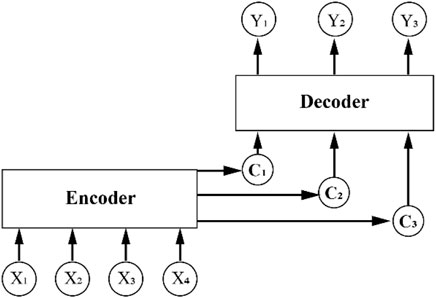
FIGURE 5. The architecture of Encoder-Decoder-Attention.

3 The design of TSTM

3.1 Domain knowledge

The introduction of domain knowledge is helpful to the application of deep learning algorithms to modeling. For pollutant concentration prediction, it is necessary to know which factors actually affect concentration, and then proper methods are applied to learn their correlations.

3.1.1 Pollution source

Type and property of air pollutant are decided by pollution source, so comprehensive information of pollution source is crucial in pollutant concentration forecast. Air pollution sources of a city can be divided into two categories from the perspective of source apportionment, namely internal source and external source, which refer to local emission and regional transmission respectively.

For local generation, it is necessary to consider the primary emission and secondary generation of pollutants. The pollutant directly discharged into the air by the pollution source and whose physical and chemical properties has not changed is primary pollutant (Xue et al., 2020). The primary pollutant is usually affected by the emission source with obvious periodicity, and the high-time resolution monitoring data of pollutant contain the change law of the emission of pollution source. For example, the bimodal mode of NO₂ hourly concentration in city corresponds to the morning and evening peak of traffic. Primary pollutant can change under the influence of physical and chemical factors or react with other substances in the air to produce secondary pollutant with different properties (Drozd et al., 2018). The formation and transformation mechanism of secondary pollutant involves complex physical and chemical reactions between different pollutants, and its harm to the environment and biology is also greater than that of primary pollutant (Kong et al., 2019; Menares et al., 2020). For example, SO₂ and NO₂, as precursors, can undergo photochemical oxidation reaction and gas-solid conversion to form sulfate and nitrate, becoming secondary particles. NOx, VOCs and CO can participate in atmospheric photochemical reaction to produce O₃. In addition, particles and O₃ also have complex interactions (Chen et al., 2019). Particles reduce the solar shortwave radiation reaching the ground through absorption and scattering, thereby reducing the photochemical reaction rate of O₃. O₃ will lead to the enhancement of atmospheric oxidation, which is conducive to the formation of secondary particles. Therefore, when predicting the concentration of pollutant, we should not only pay attention to the change law of pollutant with time, but also consider the complex interaction between different pollutants.

Air pollutants can be transported over long distances across regions, making air pollution affect each other among cities. This problem is particularly prominent in area with dense cities and heavy pollution, and sometimes the contribution of regional transmission even exceeds that of local generation (Sun et al., 2017). For air pollution prevention and control, the actions of a single city cannot fundamentally solve the problem, and regional joint prevention and control is an effective way.

When carrying out urban air pollutant concentration prediction, the introduction of pollution sources should consider the primary emission, secondary generation and regional transmission of pollutants. Based on the above analysis, the predicted pollutant, the related pollutants in the same city, and the same pollutants in related cities can be used as prediction factors. The time series of the above variables are mined by deep learning algorithm to learn their complex interactions and spatial-temporal variations.

3.1.2 Meteorological condition

In addition to the root cause of pollution source, meteorological conditions are also main factors affecting the change of pollutant concentration, which is mainly reflected in the migration and transformation process of pollutant (Dong et al., 2020). Diffusion condition represents the ability of the atmosphere to dilute, diffuse, accumulate and remove air pollutants. Under different diffusion conditions, even the same pollution source will cause significant differences in pollutant concentration (Liu et al., 2019). Wind speed, temperature, humidity and weather phenomenon are the main meteorological factors that determine the diffusion condition (Wang et al., 2019; Jury, 2020; Pérez et al., 2020; The Standardization administration of China, 2022). The wind can transport pollutant along the horizontal direction, and the wind speed determines the speed and distance of pollutant migration. The irregular change of wind will form turbulence, which will fully mix the pollutant with the surrounding clean air and promote the dilution and diffusion of pollutant. However, excessive wind speed will also blow the dust on the ground into the air, causing particle pollution. The temperature and humidity of the atmosphere are closely related to the stability of the atmosphere and affect the vertical diffusion of pollutant. At the same time, high temperature and humidity are conducive to the photochemical reaction of ozone and the hygroscopic growth of particles, respectively. Precipitation is an important way to remove air pollutants. During the falling process, raindrops absorb solid particles through collision, and gaseous pollutants can also be dissolved in water or chemically reacted with water and brought to the ground.

Referring to the instruction of the “Air pollution diffusion condition index” from the China Meteorological Administration⁴ and above research, the change of air pollutant concentration is closely related to wind speed, temperature, relative humidity and precipitation. Therefore, in the prediction of urban air pollutant concentration, the above four meteorological elements in the same city are introduced as prediction factors.

3.2 Data preprocessing

The problem of missing data is common but always overlooked. For the data-driven deep learning model, its performance is directly related to the integrity and accuracy of data. Deletion or simple interpolation method is incompetent for the data of air pollutant and meteorological element which are highly nonlinear and nonstationary. Thus, the dataset is processed by advanced Expectation Maximization (EM) algorithm. EM (Neal and Hinton, 1998) algorithm is an iterative algorithm to calculate maximum likelihood estimation of posterior distribution in the case of incomplete data. Two steps are performed alternately in each iteration cycle: E step (Expectation), calculate the conditional expectation of log likelihood function by the estimated parameters from previous iteration; M step (Maximization), maximize the log likelihood function to determine the parameters which are used in next iteration. The algorithm iterates between E step and M step until convergence. It has good convergence and is suitable for large sample.

The normalization of data is an important procedure of deep learning, which can eliminate the influence of magnitude among different features and further improve convergence speed and accuracy of model. So Min-Max normalization is applied to input data and then output data are processed by reverse normalization for the evaluation of model’s performance (Jin et al., 2015).

3.3 Feature selection

For the prediction of air pollutant concentration, based on the domain knowledge of Atmospheric Sciences, the preliminary features are conventional air pollutants (PM_2.5, PM₁₀, CO, NO₂, SO₂, O₃) and meteorological elements (wind speed, temperature, relative humidity, precipitation) of all cities in the region. In order to eliminate irrelevant features and improve computational efficiency, effective features are further selected through statistical methods. For pollution source, besides predicted pollutant itself, Spearman rank correlation coefficient and Pearson correlation coefficient are used to screen the related pollutants in the same city and the related cities on the same pollutant, and the threshold value is 0.6 (strong correlation). For meteorological condition, four meteorological elements of the same city are selected as effective features to predict pollutant concentration.

Feature decomposition and combination are used in this study. From the perspective of deep learning, the predicted pollutant, the related cities on the same pollutant, the related pollutants in the same city and the meteorological elements in the same city can be classified into four types of features: time, space, type and meteorology. Pollution source and meteorological condition are the two main factors that determine the change of pollutant concentration. Pollution source can be learned based on the first three types of features. With reference to the “Grades of air pollution diffusion meteorological conditions (QX/T 413-2018)” issued by the China Meteorological Administration, the meteorological condition in the future can be estimated based on the historical data of air pollutant concentration and meteorological elements without considering the pollution source (China Meteorological Administration, 2022). Therefore, meteorological condition can be learned based on time and meteorology features. In this study, the features of pollution source and meteorological condition are studied and predicted respectively, and then the final prediction result are obtained by integrating the two features. In addition, the hourly concentration of air pollutant has significant diurnal variation (24 h), so the time lag is 24, which is also consistent with previous studies (Wang et al., 2020). Finally, the sliding time window algorithm is applied to divide the data, and the original time series is transformed into supervised learning tasks.

3.4 Forecast strategy

On the basis of domain knowledge of atmospheric science, deep learning algorithms are employed to learn pollution source and meteorological condition, which contain time, space, type and meteorology features, namely four important correlations. Time correlation: air pollutant concentration has prominent periodicity and hourly monitoring data can reflect this variation over time. Space correlation: air pollution of different cities affects each other because of regional transmission, and Pearson correlation coefficient is used to select highly related cities for target city on the same pollutant. Type correlation: in view of the transformation mechanism of secondary pollutant, it is necessary to learn complex interactions among air pollutants, and Spearman’s rank correlation coefficient is used to find highly related pollutants for target pollutant. Meteorology correlation needs to be considered in forecast too. Attention mechanism can give each variable distinct weight, so integrated model CNN-BiLSTM-Attention with advantages of different deep learning algorithms is applied to learn and forecast pollution source (time, space, type) and meteorological condition (time, meteorology) features respectively. And then the advanced ConvLSTM is adopted to integrate the two features to forecast air pollutant concentration. Moreover, in this study multiple-output strategy is employed to obtain multistep prediction results simultaneously, which has greater efficiency and lower cost when compared with recursive strategy or multi-independent models.

3.5 Performance evaluation

Besides pollutant concentration, the forecast performance of model for air quality and heavy pollution weather are also evaluated to form a comprehensive evaluation plan.

3.5.1 Pollutant concentration forecast

TSTM’s performance is evaluated by three representative indicators including normalized mean bias (NMB), root mean square error (RMSE), and correlation coefficient (r). The prediction performance of the model is evaluated from the deviation, error and correlation between the predicted value and the observed value. Their equations are as follows:

$NMB=\frac{{\displaystyle \sum }_{i=1}^n\left(X_i-Y_i\right)}{{\sum }_{i=1}^n{Y}_i}(1)$

$RMSE=\sqrt{\frac{1}{n}{\displaystyle \sum }_{i=1}^n{\left(X_i-Y_i\right)}^2}(2)$

$r=\frac{{\displaystyle \sum }_{i=1}^n\left(X_i-\overline{X}\right)\left(Y_i-\overline{Y}\right)}{\sqrt{{\displaystyle \sum }_{i=1}^n{\left(X_i-\overline{X}\right)}^2}\sqrt{{\displaystyle \sum }_{i=1}^n{\left(Y_i-\overline{Y}\right)}^2}}(3)$

where $X_i$ and $Y_i$ are the predicted value and observed value of air pollutant concentration; $n$ is the number of test samples; $\overline{X}$ and $\overline{Y}$ are the average value of the predicted value and the observed value respectively.

3.5.2 Air quality forecast

1) Air quality index range

Based on the predicted concentrations of six conventional air pollutants, the predicted value of AQI is calculated, and that it plus/minus 25% is taken as the prediction range. If the actual value of AQI is within the prediction range, the prediction is accurate. The calculation equation of prediction accuracy of AQI range is as follow:

$A_{AQI}=\frac{n_{AQI}}{N}(4)$

Where $A_{AQI}$ is the prediction accuracy of AQI range; $n_{AQI}$ is the number of samples with accurate AQI range prediction; $N$ is the total number of samples.

2) Air quality level

The range of predicted air quality level can be obtained through AQI prediction range. If the actual value of the level is within the prediction range, the prediction is accurate. The calculation equation of the prediction accuracy of the air quality level is as follow:

$A_{AQL}=\frac{n_{AQL}}{N}(5)$

Where $A_{AQL}$ is the prediction accuracy of air quality level; $n_{AQL}$ is the number of samples with accurate air quality level prediction; $N$ is the total number of samples.

3) Chief pollutant

When the actual air quality level is greater than or equal to level II, if the prediction is the same as the actual chief pollutant, the prediction is accurate. The calculation equation of the prediction accuracy of the chief pollutant is as follow:

$A_{CP}=\frac{n_{CP}}{N}(6)$

Where $A_{CP}$is the prediction accuracy of chief pollutants; $n_{CP}$ is the number of samples with accurate chief pollutant prediction in the evaluation period; $N$ is the number of samples whose actual air quality level is greater than or equal to level II.

3.5.3 Heavy pollution weather forecast

1) Prediction accuracy

The prediction accuracy of air quality level when the actual AQI is greater than 200 is calculated as follow:

${HA}_{AQL}=\frac{n_{AQL}}{N_{OH}}(7)$

Where ${HA}_{AQL}$ is the prediction accuracy of heavy pollution weather; $n_{AQL}$ is the number of samples with accurate prediction in the evaluation period; $N_{OH}$ is the actual number of heavy pollution weather samples.

2) Prediction test score

The prediction accuracy of air quality level when the predicted or actual AQI is greater than 200 is calculated as follow:

${HS}_{AQL}=\frac{n_{AQL}}{N_{FOH}}(8)$

Where ${HS}_{AQL}$ is the prediction test score of heavy pollution weather; $n_{AQL}$ is the number of samples with accurate prediction in the evaluation period; $N_{FOH}$ is the number of predicted or actual heavy pollution weather samples.

Based on above all, we proposed a novel integrated model TSTM based on the theory and methods of Atmospheric Sciences and deep learning for regional and multistep air quality forecast. The architecture and workflow of TSTM can be seen in Figure 6 and Figure 7, respectively.

FIGURE 6

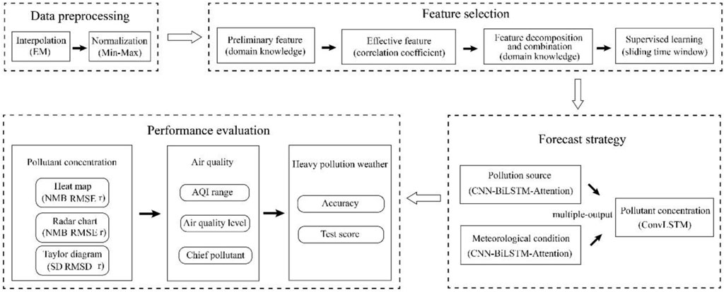
FIGURE 6. The architecture of TSTM.

FIGURE 7

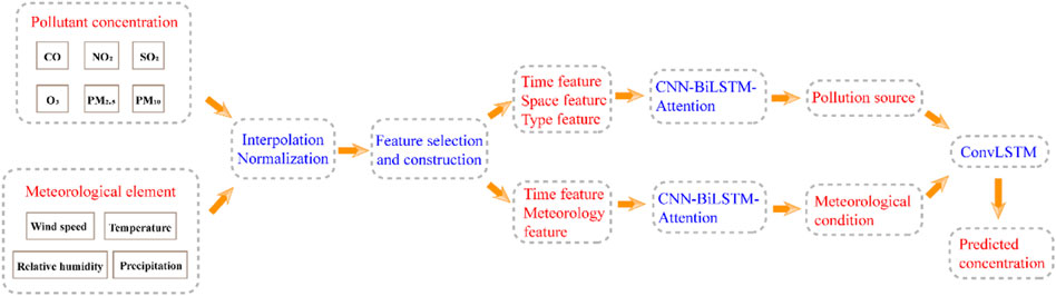
FIGURE 7. The workflow of TSTM.

4 Results and discussion

4.1 Pollutant concentration forecast

The performance of TSTM for regional (e.g. BJ and TJ) and multistep (e.g. CO_1, CO_2 and CO_3) air quality prediction is tested on the hourly concentrations of six conventional air pollutants in study area, and independent test sets (e.g. BJ 1 and BJ 2) are used. In view of a large number of experimental results, the heat map is used to present the performance of TSTM on all cities and pollutants. NMB in Figure 8 reflects the deviation between prediction and observation. A positive value indicates that the predicted concentration is generally higher than actual concentration, while a negative value indicates that the predicted result is lower. According to all results, the number of positive values is equal to that of negative values. Generally, the NMB does not show obvious correlation with city, pollutant, prediction step and test set, and there is no systematical deviation shown by these experiments.

FIGURE 8

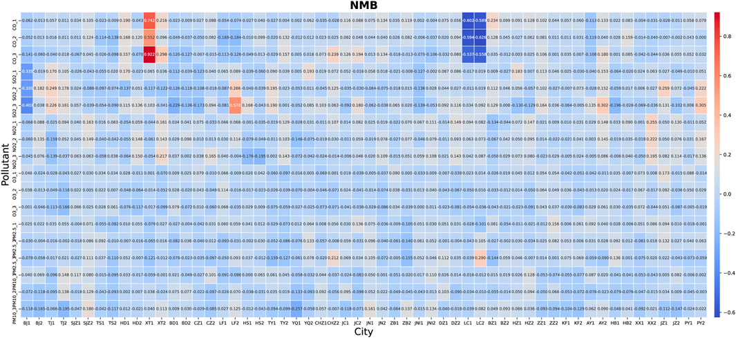
FIGURE 8. The NMB of pollutant concentration prediction of TSTM in “2+26” cities.

Figure 9 shows the RMSE of TSTM under different conditions. RMSE can not only reflect the average error of the prediction, but also is very sensitive to outliers, which is the focus of deep learning in the application for air quality prediction. The experimental results show a certain regularity. The accuracy of the model is mainly affected by the data themselves. Generally, the higher the concentration value, the higher the RMSE value. On test set 1, the six conventional air pollutants are arranged according to the increasing order of the average concentration value, namely CO, SO₂, NO₂, O₃, PM_2.5 and PM₁₀, which is consistent with the order of RMSE value. For 1-step prediction, the results of PM₁₀ on test set 1 show that the RMSE and concentration of Shijiazhuang is 46.83 μg/m³ and 194 μg/m³, while the 19.49 μg/m³ and 138 μg/m³ of Jining. In Anyang, the concentration of PM_2.5 on test set 1 and 2 are 162 μg/m³ and 36 μg/m³ respectively, while the RMSE are 28.62 μg/m³ and 5.07 μg/m³. For multistep prediction, based on the same historical data, it is obviously more difficult to predict multistep result at the same time than one-step result. The experimental results show that the accuracy decreases slightly with the increase of prediction steps. Take the O₃ on test set 2 as an example, in Taiyuan, the RMSE of 1 step, 2 steps and 3 steps are 16.67 μg/m³, 17.42 μg/m³ and 19.35 μg/m³ respectively.

FIGURE 9

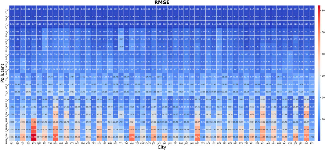
FIGURE 9. The RMSE of pollutant concentration prediction of TSTM in “2+26” cities (unit: mg/m³ for CO, μg/m³ for other pollutants).

Figure 10 shows the correlation between the predicted value and the actual value, that is, whether the model can accurately capture the change trend of air pollution. The results show that TSTM has a good performance in almost all experiments. The predicted value is strongly correlated with the actual value (r > 0.6), and the correlation coefficient decreases slightly with the increase of prediction steps. Very few experimental results show weak correlation, the pollutants with low concentration value such as CO and SO₂ are further explored. There are random deviations from deep learning model. Compared with pollutants with high concentration value, the correlation of pollutants with low concentration value are more affected, but the uncertainty only exists in very few cases.

FIGURE 10

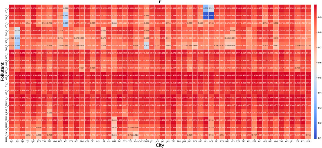
FIGURE 10. The r of pollutant concentration prediction of TSTM in “2+26” cities.

In view of a large number of experimental results and similar forecast effects in all cities, it is necessary to select representative city and further carry out detailed comparative analysis. Beijing is the capital of China and has an important strategic position, but it is under considerable strain in air pollution prevention and control. Beijing is also the central city of this study area, and it is a common target in previous studies. Therefore, Beijing is selected as the representative, and the radar chart is used to analyze the prediction effects of TSTM in all experiments.

Figure 11 shows the results of TSTM’s multistep prediction for six conventional air pollutants in Beijing, involving three evaluation indicators (NMB, RMSE, r) and two independent test sets (winter and summer). TSTM adopts the multi-output strategy for multistep prediction, and the prediction error usually increases with the increase of prediction step. In addition, the random deviation is shown by NMB.

FIGURE 11

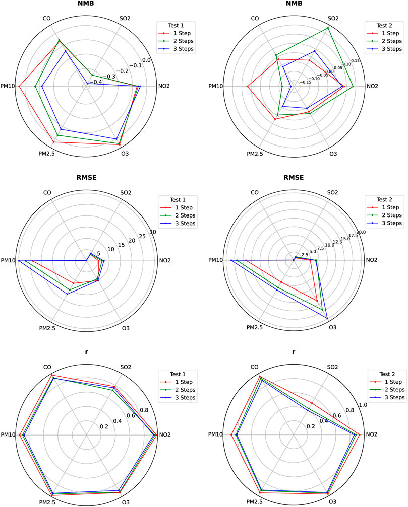
FIGURE 11. The radar chart of pollutant concentration prediction of TSTM in Beijing.

In winter (Test 1), the air pollution is relatively heavier and there are more negative values of NMB. The NMB of high concentration value PM₁₀ (72.19 μg/m³) and PM_2.5 (51.76 μg/m³) increases with the increase of prediction step. For medium concentrations value of O₃ (44.70 μg/m³) and NO₂ (33.80 μg/m³), the NMB for one-step and two-steps prediction are close, while the NMB of three-steps decreases. The NMB of low concentration value SO₂ (6.33 μg/m³) and CO (0.79 mg/m³) for one-step and two-steps prediction are close, while the NMB of three-steps increases. In summer (Test 2), except for the increased concentration of O₃, the concentration of other pollutants decreases, and the number of positive and negative values of NMB are approximate. The NMB of high concentration value PM₁₀ (52.82 μg/m³) increases with the increase of prediction step; The NMB of high concentration value O₃ (102.78 μg/m³), medium concentration value PM_2.5 (36.35 μg/m³) and low concentration value CO (0.66 mg/m³) first decrease and then increase with the increase of prediction step. The NMB of lower concentration values of NO₂ (26.05 μg/m³) and SO₂ (2.70 μg/m³) first increase and then decrease with the increase of prediction step. Compared with NMB, the laws of RMSE and r of model are more obvious. Considering the current air pollution in China, CO and SO₂ are not the main pollutants, while O₃ (summer) and PM (winter) pollution are more serious, that is, they have higher frequency of pollution process (maximum value of concentration). The weak ability to predict the peak value of data is a common problem for models based on machine learning. And it can be seen from Figure 11 that the RMSE value of PM₁₀, PM_2.5 and O₃ is always greater than that of the other three pollutants. In general, RMSE value increases with the increase of pollutant concentration value and prediction step. r decreases with the increase of prediction step, and is affected by random deviation. For the same pollutant, r is positively correlated with the concentration.

Taylor diagram can compare the performance of multiple models from different aspects in single map (Taylor, 2001). It is recommended by Intergovernmental Panel on Climate Change (IPCC) and is widely favored in the field of Geoscience. Taylor diagram skillfully presents the cosine relationship of the three evaluation indicators of the model, namely, the central root mean square difference (RMSD), standard deviation and correlation coefficient. In this study, this data visualization method is applied for model comparison.

The traditional root mean square error $E$ can be decomposed into overall deviation $\overline{E}$and central root mean square difference $E^{\prime }$. The smaller the $E^{\prime }$, the better the prediction precision.

$E={\left[\frac{\mathrm{1}}{N}{\displaystyle \sum }_{n=\mathrm{1}}^N{\left(f_n-r_n\right)}^{\mathrm{2}}\right]}^{1/\mathrm{2}}(9)$

$\overline{E}=\overline{f}-\overline{r}(10)$

$E^{\prime }={\left\{\frac{\mathrm{1}}{N}{\displaystyle \sum }_{n=\mathrm{1}}^N{\left[\left(f_n-\overline{f}\right)-\left(r_n-\overline{r}\right)\right]}^{\mathrm{2}}\right\}}^{1/\mathrm{2}}(11)$

$E^{\mathrm{2}}={\overline{E}}^{\mathrm{2}}+{E^{\prime }}^{\mathrm{2}}(12)$

Where $N$ is the number of samples; $f_n$ and $r_n$ are the predicted and actual value of the $n$th sample; $\overline{f}$ and $\overline{r}$ are the average of the predicted sequence and the actual sequence.

The standard deviation $\sigma$ can be used to judge whether the prediction sequence of the model reflects the dispersion of the actual sequence.

${\sigma }_A={\left[\frac{\mathrm{1}}{N}{\displaystyle \sum }_{n=\mathrm{1}}^N{\left(A_n-\overline{A}\right)}^{\mathrm{2}}\right]}^{\mathrm{1}/\mathrm{2}}(13)$

Where $A_n$ and $\overline{A}$ are the $n$th value and average value of the sequence respectively.

The closer the correlation coefficient $R$ is to 1, the better the prediction performance of the model.

$R=\frac{\frac{\mathrm{1}}{N}{\displaystyle \sum }_{n=\mathrm{1}}^N\left(f_n-\overline{f}\right)\left(r_n-\overline{r}\right)}{{\sigma }_f{\sigma }_r}(14)$

Where $f_n$ and $r_n$ are the predicted and actual value of the $n$th sample; $\overline{f}$ and $\overline{r}$ are the average of the forecast sequence and the actual sequence; ${\sigma }_f$and ${\sigma }_r$ are the standard deviation of the forecast sequence and the actual sequence.

Three indicators can form a cosine relationship:

${E^{\prime }}^{\mathrm{2}}={\sigma }_f^{\mathrm{2}}+{\sigma }_r^{\mathrm{2}}-\mathrm{2}{\sigma }_f{\sigma }_{r}R(15)$

$c^{\mathrm{2}}=a^{\mathrm{2}}+b^{\mathrm{2}}-\mathrm{2}abcos\varphi (16)$

Referring to the “Technical guide for ambient air quality prediction and early-warning methods” from the China National Environmental Monitoring Centre (China National Environmental Monitoring Centre, 2017), three classical benchmark models, Radial basis function network (RBF) of traditional machine learning, Deep Belief Network (DBN) and Elman neural network (Elman) of deep learning, are selected to compare with the proposed model TSTM.

Figure 12 and Figure 13 are Taylor diagrams of the prediction performance of four models on two test sets in Beijing. The results of Test 1 show that they are TSTM, Elman, RBF and DBN in descending order according to the prediction accuracy. Although the deep learning model has more complex structure and algorithm, it does not mean that it must obtain better effect than traditional machine learning. It is necessary to explore the applicability of different deep learning algorithms by practice, and establish an effective model for air quality prediction. In this study, DBN cannot capture the characteristics of high oscillation of air pollutant concentration, and its three indicators of all pollutants are poor. RBF has worse robustness, and the prediction accuracy is obviously affected by outlier (PM₁₀). Elman belongs to recurrent neural network and has short-term memory ability. Its prediction effect for most pollutants is second only to TSTM, but it has the same problem as RBF. TSTM not only combines CNN, BiLSTM and other advanced deep learning algorithms suitable for time series prediction, but also considers varieties of related features based on domain knowledge. As shown in experiments, TSTM obtains better results especially in the face of outliers. In addition, the multistep effects of recurrent neural network TSTM and Elman with memory ability are generally more stable, and the prediction error increases slightly with the increase of prediction step.

FIGURE 12

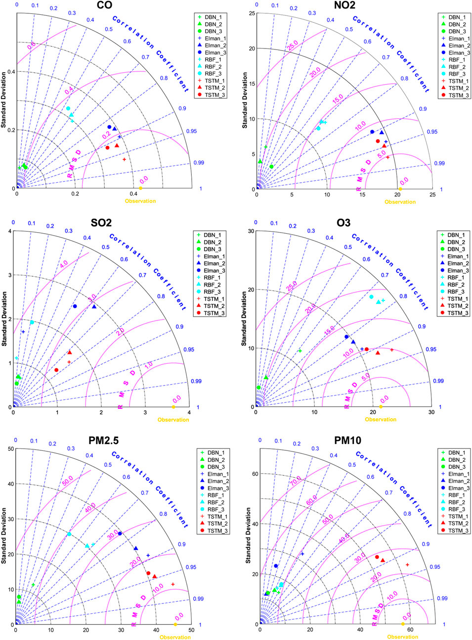
FIGURE 12. The Taylor diagram of pollutant concentration prediction in Beijing (Test 1).

FIGURE 13

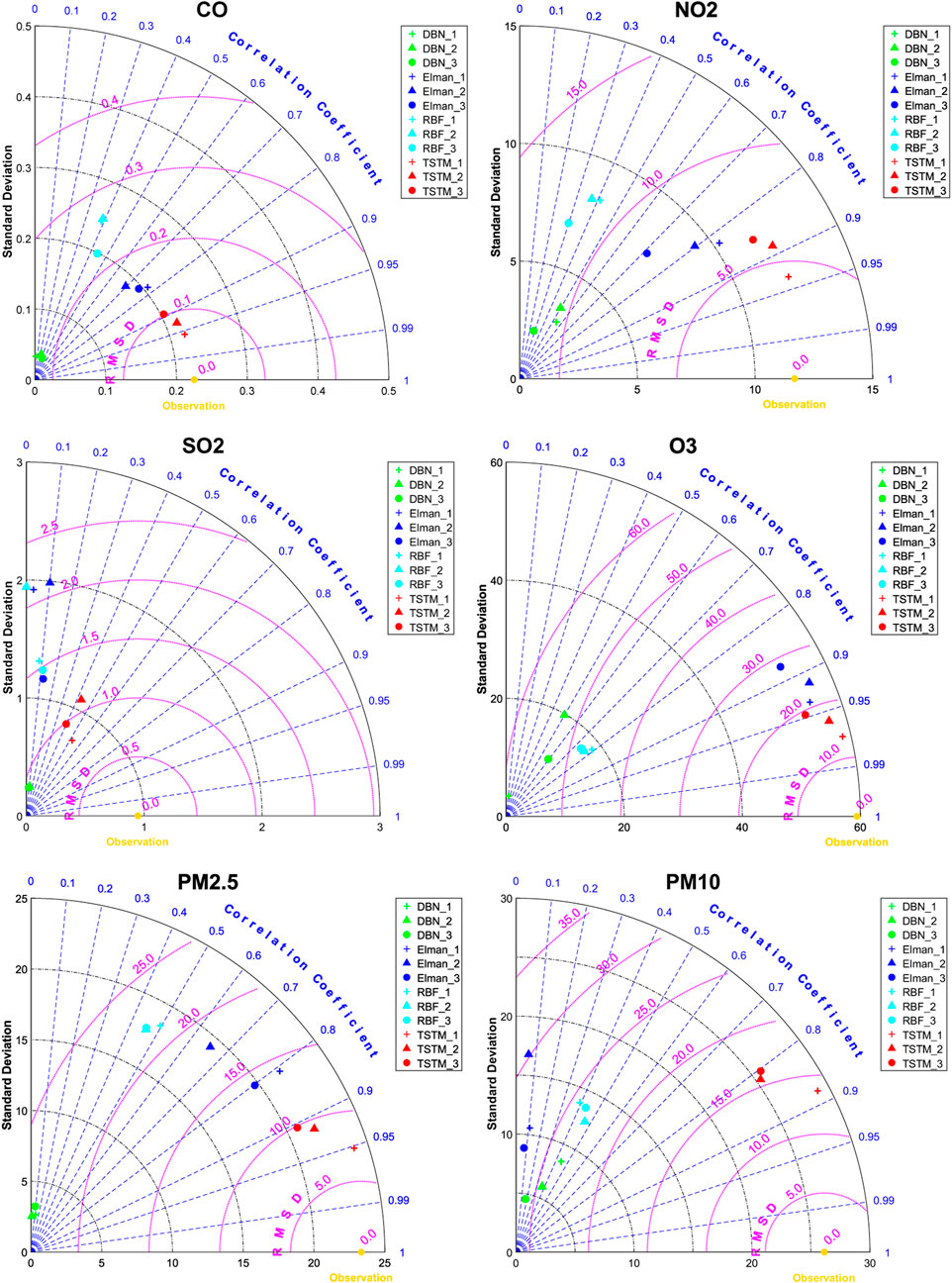
FIGURE 13. The Taylor diagram of pollutant concentration prediction in Beijing (Test 2).

The experimental results of Test 2 are similar to that of Test 1. TSTM still maintains the highest precision. Take PM_2.5 in winter and O₃ in summer as examples, the RMSD (r) of the three-steps prediction are 16.52 μg/m³ (0.93) and 19.31 μg/m³ (0.95) respectively. The experimental results show that TSTM has good robustness and generalization ability.

4.2 Air quality forecast

The purpose of pollutant concentration prediction is to release air pollution information in advance, providing the guidance for the public in production and life as well as the basis for government in pollution prevention and control. Therefore, based on the predicted concentration of six conventional air pollutants, the performance of four models for air quality forecast is further compared and analyzed according to the “Technical Regulation on Ambient Air Quality Index (HJ 633-2012)” issued by the Ministry of Ecology and Environment of China (The Ministry of Ecology and Environment of China, 2022b). Table 1 reflects the accuracy of the four models for different tasks of air quality prediction. According to the “Technical guideline for numerical forecasting of ambient air quality (HJ 1130-2020)”, the requirement for air quality level is 60%, which can be used as a reference. The results show that there is a large gap in the performance of the four models for air quality prediction. RBF and DBN have similar prediction accuracy for AQI range and air quality level, but DBN has poor prediction effect for chief pollutant. TSTM and Elman with recurrent neural network structure always rank in the top two. Their effects of multistep prediction are more stable, and the accuracy decreases slightly with the increase of steps. The accuracy of one-step prediction of the three benchmark models are all lower than 0.6, but the performance of TSTM is the best, reaching 0.88. The accuracy for air quality level of the four models can all meet the national requirement. TSTM has the best performance, its one-step and three-steps prediction can reach 0.98 and 0.92, respectively.

TABLE 1

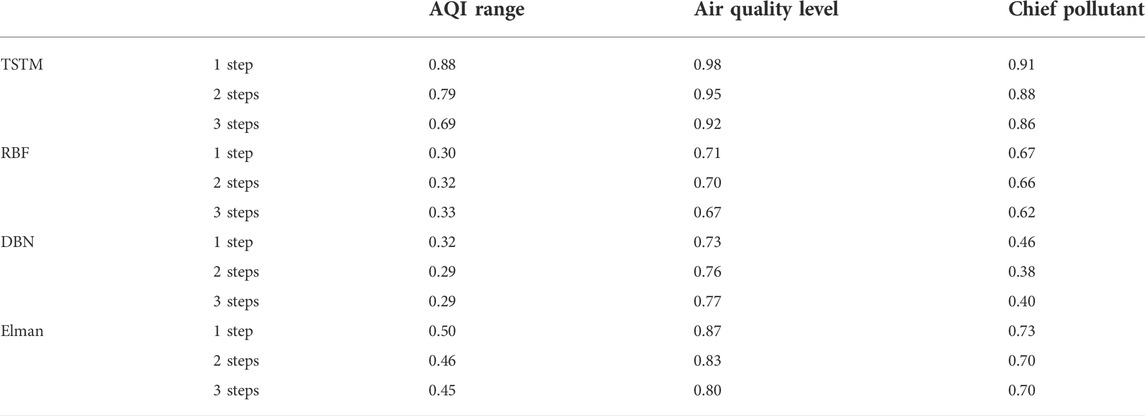
TABLE 1. Accuracy of four models for air quality forecast in Beijing.

4.3 Heavy pollution weather forecast

For air pollution prevention and control, heavily polluted weather has always been the focus of attention. In order to reduce pollution and protect human health, all cities issue the emergency plan for heavy air pollution and take measures according to the air quality forecast results. Therefore, it is crucial to ensure the prediction accuracy in heavy pollution weather. At the same time, the prediction ability for peak values has always been a difficulty and challenge for machine learning model, and the heavy pollution weather contains more concentration maximum values, which is a “touchstone” to test the robustness of the model. Table 2 reveals great differences of the four models under extreme conditions. Deep learning has a higher upper limit than traditional machine learning, and the prediction accuracy of RBF for heavy pollution weather is lower than that of three deep learning models. Elman still maintains the second position. However, with the increase of prediction steps, the performance decreases significantly, and the accuracy for air quality level of three-steps prediction is lower than 0.6. TSTM widens the gap with other models in heavy pollution weather forecast. The accuracy and test score of one-step prediction are close to the full score, although the performance decreases slightly with the steps, the results of three-steps prediction are also above 0.86.

TABLE 2

TABLE 2. Performance of four models for heavy pollution weather forecast in Beijing.

5 Conclusion

Accurate prediction of pollutant concentration is significant to air pollution prevention. To overcome the shortcomings of present studies, a novel integrated model TSTM is proposed to achieve regional and multistep air quality prediction. The domain knowledge of Atmospheric Sciences is innovatively introduced to design the model architecture, and advanced deep learning algorithms including ConvLSTM, Seq2Seq, etc. are applied to learn important correlations of time, space, type, meteorology. “Beijing-Tianjin-Hebei air pollution transmission channel (2+26 cities)" is selected as the study area, and the prediction of hourly concentrations for six conventional air pollutants in all cities are carried out. And then the detailed performance evaluation and analysis are conducted based on two independent test sets (winter and summer) and three benchmark models (RBF, DBN, Elman).

Pollutant concentration prediction results show that TSTM has small NMB and RMSE as well as large r, which is similar in all cities. As for air quality prediction, there are similar prediction effects as pollutant concentration prediction. TSTM is obviously better than other comparison models, and the prediction accuracy only decreases slightly with the increase of prediction step. The tests under heavy pollution weather show that TSTM and Elman with recurrent neural network structure have better results, but the accuracy of Elman with short-term memory decreases significantly with the increase of prediction step. In general, comprehensive experiments and detail evaluations prove TSTM’s feasibility on regional and multistep air quality prediction especially in heavy pollution weather. In future, we will continue improving our model, which is hoped to provide effective supports for the daily health guide of the public and the air pollution control of government.

Data availability statement

The data can be downloaded from http://www.cma.gov.cn/ and http://www.mee.gov.cn. Basic models can be called from the Keras of Python. And other materials will be provided when requested.

Author contributions

All authors listed have made a substantial, direct, and intellectual contribution to the work and approved it for publication.

Funding

This work was supported by the Scientific Research Fund of Hainan University (grant number: KYQD (ZR)-22097, KYQD (ZR)-22096).

Conflict of interest

The authors declare that the research was conducted in the absence of any commercial or financial relationships that could be construed as a potential conflict of interest.

Publisher’s note

All claims expressed in this article are solely those of the authors and do not necessarily represent those of their affiliated organizations, or those of the publisher, the editors and the reviewers. Any product that may be evaluated in this article, or claim that may be made by its manufacturer, is not guaranteed or endorsed by the publisher.

Footnotes

¹https://www.nsfc.gov.cn/publish/portal0/tab934/info79588.htm.

²https://www.mee.gov.cn/

³http://www.cma.gov.cn/

⁴http://www.cma.gov.cn/2011qxfw/2011qqxkp/2011qqxzs/201110/t20111027_126331.html.

References

Bahdanau, D., Cho, K., and Bengio, Y. (2014). Neural machine translation by jointly learning to align and translate[J]. arXiv preprintarXiv:1409.0473).

Google Scholar

Chakma, A., Vizena, B., Cao, T., Lin, J., and Zhang, J. (2017). “Image-based air quality analysis using deep convolutional neural network[C],” in 2017 IEEE international conference on image processing (ICIP), 17-20 sept, 3949–3952.

Google Scholar

Chen, J., Shen, H., Li, T., Peng, X., Cheng, H., and Ma, C. (2019). Temporal and spatial features of the correlation between PM2.5 and O3 concentrations in China. Int. J. Environ. Res. Public Health 16 (23), 4824. doi:10.3390/ijerph16234824

PubMed Abstract | CrossRef Full Text | Google Scholar

Chen, Y. (2018). Prediction algorithm of PM2.5 mass concentration based on adaptive BP neural network. Computing 100 (8), 825–838. doi:10.1007/s00607-018-0628-3

CrossRef Full Text | Google Scholar

Cheng, F., Feng, C., Yang, Z., Hsu, C. H., Chan, K. W., Lee, C. Y., et al. (2021). Corrigendum to “Evaluation of real-time PM2.5 forecasts with the WRF-CMAQ modeling system and weather-pattern-dependent bias-adjusted PM2.5 forecasts in Taiwan”. Atmos. Environ. 354, 118263. doi:10.1016/j.atmosenv.2021.118263

CrossRef Full Text | Google Scholar

Cheng, Y., Zhang, H., Liu, Z., Chen, L., and Wang, P. (2019). Hybrid algorithm for short-term forecasting of PM2.5 in China[J]. Atmos. Environ. 200, 264–279.

CrossRef Full Text | Google Scholar

China Meteorological Administration. 2022. Grades of air pollution diffusion meteorological conditions. Beijing: QX/. T 413-2018) [EB/OL]. [2022-07-15] Availabla at: http://cmastd.cmatc.cn/standardView.jspx?id=2875.

Google Scholar

China National Environmental Monitoring Centre (2017). Technical guide for ambient air quality prediction and early-warning methods[M]. Beijing: China Environmental Science Press.

Google Scholar

Cho, K., Merrienboer, B. V., Gulcehre, C., Bahdanau, D., Bougares, F., Schwenk, H., et al. (2014). Learning phrase representations using RNN encoder-decoder for statistical machine translation[J]. Comput. Sci. 338, 1724–1734.

Google Scholar

Dong, Z., Wang, S., Xing, J., Chang, X., Ding, D., and Zheng, H. (2020). Regional transport in Beijing-Tianjin-Hebei region and its changes during 2014–2017: The impacts of meteorology and emission reduction. Sci. Total Environ. 737, 139792. doi:10.1016/j.scitotenv.2020.139792

PubMed Abstract | CrossRef Full Text | Google Scholar

Drozd, G. T., Zhao, Y., Saliba, G., Frodin, B., Maddox, C., Oliver Chang, M. C., et al. (2018). Detailed speciation of intermediate volatility and semivolatile organic compound emissions from gasoline vehicles: Effects of cold-starts and implications for secondary organic aerosol formation. Environ. Sci. Technol. 53 (3), 1706–1714. doi:10.1021/acs.est.8b05600

CrossRef Full Text | Google Scholar

Hochreiter, S., and Schmidhuber, J. (1997). Long short-term memory. Neural Comput. 9 (8), 1735–1780. doi:10.1162/neco.1997.9.8.1735

PubMed Abstract | CrossRef Full Text | Google Scholar

Ian, G., Yoshua, B., and Aaron, C. (2017). Deep learning[M]. MIT Press.

Google Scholar

Jerrett, M. (2015). Atmospheric science: The death toll from air-pollution sources[J]. Nature 525 (7569), 330–331. doi:10.1038/525330a

PubMed Abstract | CrossRef Full Text | Google Scholar

Jin, J., Li, M., and Jin, L. (2015). Data normalization to accelerate training for linear neural net to predict tropical cyclone tracks. Math. Problems Eng. 2015, 1–8. doi:10.1155/2015/931629

CrossRef Full Text | Google Scholar

Jury, M. R. (2020). Meteorology of air pollution in los angeles. Atmos. Pollut. Res. 11 (7), 1226–1237. doi:10.1016/j.apr.2020.04.016

CrossRef Full Text | Google Scholar

Kim, K., Kim, D., Noh, J., and Kim, M. (2018). Stable forecasting of environmental time series via long short term memory recurrent neural network. IEEE Access 6, 75216–75228. doi:10.1109/access.2018.2884827

CrossRef Full Text | Google Scholar

Kong, L., Hu, M., Tan, Q., Feng, M., Qu, Y., An, J., et al. (2019). Key role of atmospheric water content in the formation of regional haze in southern China. Atmos. Environ. 216, 116918. doi:10.1016/j.atmosenv.2019.116918

CrossRef Full Text | Google Scholar

Lecun, Y. (1989). Generalization and network design strategies[J]. Connect. perspective 19.

Google Scholar

Li, T., Wang, Y., and Yuan, Q. (2020). Remote sensing estimation of regional NO2 via space-time neural networks. Remote Sens. 12, 2514. doi:10.3390/rs12162514

CrossRef Full Text | Google Scholar

Li, X., Jin, L., and Kan, H. (2019). Air pollution: A global problem needs local fixes. Nature 570 (7762), 437–439. doi:10.1038/d41586-019-01960-7

PubMed Abstract | CrossRef Full Text | Google Scholar

Liu, Z., Wang, H., Shen, X., Peng, Y., Shi, Y., Che, H., et al. (2019). Contribution of meteorological conditions to the variation in winter PM2.5 concentrations from 2013 to 2019 in middle-eastern China. Atmosphere 10 (10), 563. doi:10.3390/atmos10100563

CrossRef Full Text | Google Scholar

Menares, C., Gallardo, L., Kanakidou, M., Seguel, R., and Huneeus, N. (2020). Increasing trends (2001–2018) in photochemical activity and secondary aerosols in Santiago, Chile. Tellus B Chem. Phys. Meteorology 72 (1), 1821512–1821518. doi:10.1080/16000889.2020.1821512

CrossRef Full Text | Google Scholar

Mo, X., Li, H., Zhang, L., and Qu, Z. (2020). A novel air quality evaluation paradigm based on the fuzzy comprehensive theory. Appl. Sci. (Basel). 10 (23), 8619. doi:10.3390/app10238619

CrossRef Full Text | Google Scholar

Mo, X., Li, H., Zhang, L., and Qu, Z. (2021). Environmental impact estimation of PM2.5 in representative regions of China from 2015 to 2019: Policy validity, disaster threat, health risk, and economic loss. Air Qual. Atmos. Health 14 (10), 1571–1585. doi:10.1007/s11869-021-01040-8

CrossRef Full Text | Google Scholar

Mo, X., Zhang, l., Li, H., and Qu, Z. (2019). A novel air quality early-warning system based on artificial intelligence. Int. J. Environ. Res. Public Health 16 (19), 3505. doi:10.3390/ijerph16193505

PubMed Abstract | CrossRef Full Text | Google Scholar

Mu, L., Su, J., Mo, X., Peng, N., Xu, Y., Wang, M., et al. (2021). The temporal-spatial variations and potential causes of dust events in xinjiang basin during 1960–2015. Front. Environ. Sci. 9, 727844. doi:10.3389/fenvs.2021.727844

CrossRef Full Text | Google Scholar

Neal, R. M., and Hinton, G. E. (1998). “A view of the em algorithm that justifies incremental, sparse, and other variants[M],” in Learning in graphical models.(Dordrecht: Springer Netherlands), 355–368.

CrossRef Full Text | Google Scholar

Ng, K. Y., and Awang, N. (2018). Multiple linear regression and regression with time series error models in forecasting PM10 concentrations in Peninsular Malaysia. Environ. Monit. Assess. 190 (2), 63. doi:10.1007/s10661-017-6419-z

PubMed Abstract | CrossRef Full Text | Google Scholar

Pak, U., Ma, J., Ryu, U., Ryom, K., Juhyok, U., Pak, K., et al. (2020). Deep learning-based PM2.5 prediction considering the spatiotemporal correlations: A case study of beijing, China. Sci. Total Environ. 699, 133561. doi:10.1016/j.scitotenv.2019.07.367

PubMed Abstract | CrossRef Full Text | Google Scholar

Pérez, I. A., García, M., Sánchez, M. L., Pardo, N., and Fernández-Duque, B. (2020). Key points in air pollution meteorology. Int. J. Environ. Res. Public Health 17 (22), 8349. doi:10.3390/ijerph17228349

CrossRef Full Text | Google Scholar

Perišić, M., Maletić, D., Stojić, S. S., Rajšić, S., and Stojić, A. (2017). Forecasting hourly particulate matter concentrations based on the advanced multivariate methods. Int. J. Environ. Sci. Technol. (Tehran). 14 (5), 1047–1054. doi:10.1007/s13762-016-1208-8

CrossRef Full Text | Google Scholar

Pohoata, A., and Lungu, E. (2017). A complex analysis employing ARIMA model and statistical methods on air pollutants recorded in ploiesti, Romania. Rev. Chim. 68, 818–823. doi:10.37358/rc.17.4.5559

CrossRef Full Text | Google Scholar

Sahu, S. K., Sharma, S., Zhang, H., Chejarla, V., Guo, H., Hu, J., et al. (2020). Estimating ground level PM2.5 concentrations and associated health risk in India using satellite based AOD and WRF predicted meteorological parameters. Chemosphere 255, 126969. doi:10.1016/j.chemosphere.2020.126969

PubMed Abstract | CrossRef Full Text | Google Scholar

Schuster, M., and Paliwal, K. K. (1997). Bidirectional recurrent neural networks. IEEE Trans. Signal Process. 45 (11), 2673–2681. doi:10.1109/78.650093

CrossRef Full Text | Google Scholar

Shi, X., Chen, Z., Wang, H., Yeung, D-Y., Wong, W. K., and Woo, W-C. (2015). “Convolutional LSTM network: A machine learning approach for precipitation nowcasting[C],” in Proc.eedings of the 28th Int.ernational Conf.erence on Neural Inf.ormation Processing Syst.ems 06/121 (Cambridge, MA, USA: MIT Press), 802–810.

Google Scholar

Spiridonov, V., Jakimovski, B., Spiridonova, I., and Pereira, G. (2019). Development of air quality forecasting system in Macedonia, based on WRF-Chem model. Air Qual. Atmos. Health 12 (7), 825–836. doi:10.1007/s11869-019-00698-5

CrossRef Full Text | Google Scholar

Sun, J., Huang, L., Liao, H., Li, J., and Hu, J. (2017). Impacts of regional transport on particulate matter pollution in China: A review of methods and results. Curr. Pollut. Rep. 3 (3), 182–191. doi:10.1007/s40726-017-0065-5

CrossRef Full Text | Google Scholar

Taylor, K. E. (2001). Summarizing multiple aspects of model performance in a single diagram. J. Geophys. Res. 106 (D7), 7183–7192. doi:10.1029/2000jd900719

CrossRef Full Text | Google Scholar

The Ministry of Ecology and Environment of China. 2022. Technical guideline for numerical forecasting of ambient air quality. HJ 1130-2020) [EB/OL]. [2022-07-15] Availabla at: https://www.mee.gov.cn/ywgz/fgbz/bz/bzwb/jcffbz/202005/t20200518_779714.shtml.

Google Scholar

The Ministry of Ecology and Environment of China. 2022. Technical regulation on ambient air quality index. HJ 633-2012) [EB/OL]. [2022-07-15] Availabla at: https://www.mee.gov.cn/ywgz/fgbz/bz/bzwb/jcffbz/201203/W020120410332725219541.pdf.

Google Scholar

The Standardization administration of China 2022. Grades of atmospheric purification capability. GB/T 34299-2017) [EB/OL]. [2022-07-15] Availabla at: http://ah.cma.gov.cn/zfxxgk/zwgk/flfgbz/dfbz/202102/t20210210_2720010.html.

Google Scholar

Ulpiani, G., Duhirwe, P., Yun, G., and Lipson, M. (2022). Meteorological influence on forecasting urban pollutants: Long-term predictability versus extreme events in a spatially heterogeneous urban ecosystem. Sci. Total Environ. 814, 152537. doi:10.1016/j.scitotenv.2021.152537

PubMed Abstract | CrossRef Full Text | Google Scholar

United Nations Environment Programme. 2022. International Day of Clean Air for blue skies. [EB/OL].[2022-07-05] Availabla at: https://www.un.org/en/observances/clean-air-day.

Google Scholar

Wang, H., Li, X., Wang, D., Zhao, J., He, H., and Peng, Z-R. (2020). Regional prediction of ground-level ozone using a hybrid sequence-to-sequence deep learning approach. J. Clean. Prod. 253, 119841. doi:10.1016/j.jclepro.2019.119841

CrossRef Full Text | Google Scholar

Wang, P., Guo, H., Hu, J., Kota, S. H., Ying, Q., and Zhang, H. (2019). Responses of PM2.5 and O3 concentrations to changes of meteorology and emissions in China. Sci. Total Environ. 662, 297–306. doi:10.1016/j.scitotenv.2019.01.227

PubMed Abstract | CrossRef Full Text | Google Scholar

Wen, C., Liu, S., Yao, X., Peng, L., Li, X., Hu, Y., et al. (2019). A novel spatiotemporal convolutional long short-term neural network for air pollution prediction. Sci. Total Environ. 654, 1091–1099. doi:10.1016/j.scitotenv.2018.11.086

PubMed Abstract | CrossRef Full Text | Google Scholar

Xue, Y., Cao, X., Ai, Y., Xu, K., and Zhang, Y. (2020). Primary air pollutants emissions variation characteristics and future control strategies for transportation sector in beijing, China. Sustainability 12 (10), 4111. doi:10.3390/su12104111

CrossRef Full Text | Google Scholar

Yu, T., Wang, Y., Huang, J., Liu, X., Li, J., and Zhan, W. (2022). Study on the regional prediction model of PM2.5 concentrations based on multi-source observations. Atmos. Pollut. Res. 13 (4), 101363. doi:10.1016/j.apr.2022.101363

CrossRef Full Text | Google Scholar

Zhao, S., Yu, Y., Qin, D., Yin, D., Dong, L., and He, J. (2019). Analyses of regional pollution and transportation of PM2.5 and ozone in the city clusters of Sichuan Basin, China. Atmos. Pollut. Res. 10 (2), 374–385. doi:10.1016/j.apr.2018.08.014

CrossRef Full Text | Google Scholar