Traffic flow and vehicle speed monitoring with the object detection method from the roadside distributed acoustic sensing array

Distributed acoustic sensing (DAS) is an emerging technology that transforms a typical glass telecommunications cable into a network of seismic sensors. DAS may, therefore, concurrently record the vibrations of passing vehicles over tens of kilometers and shows potential to monitor traffic at a low cost with minimal maintenance. With big-data DAS recording, automatically recognizing and tracking vehicles on the road in real time still presents numerous obstacles. Therefore, we present a deep learning technique based on the unified real-time object detection algorithm to estimate traffic flow and vehicle speed in DAS data and evaluate them along a 500-m fiber length in Beijing’s suburbs. We reconstructed the DAS recordings into 1-min temporal–spatial images over the fiber section and manually labeled about 10,000 images as vehicle passing or background noise. The precision to identify the passing cars can reach 95.9% after training. Based on the same DAS data, we compared the performance of our method to that of a beamforming technique, and the findings indicate that our method is significantly faster than the beamforming technique with equal performance. In addition, we examined the temporal traffic trend of the road segment and the classification of vehicles by weight.

Introduction

Traffic monitoring and management are essential links in the construction of smart cities. Comprehensively monitoring the densely distributed urban road network is still a challenging task. Surveillance cameras are the most intuitive monitoring method, but the construction and maintenance costs are high. At the same time, video processing is enormous, and monitoring coverage has dead spots and is also greatly affected by lighting and meteorological factors. Using the cell phone signals of people on the road network is an innovation to track road congestion in real time. However, both of the aforementioned methods have personal privacy concerns, so developing new monitoring methods complements the deficiencies of the existing observation systems.

The emergence of distributed acoustic sensing (DAS) applications in the city can revolutionize the smart city’s sensing abilities as lots of dark fibers existing in the city can be transformed into vibration sensors. Because infrastructure optical cables for communication or traffic surveillance would cover almost every major road, building a DAS transport management system over the whole city will be possible with the benefits of fast construction and low maintenance cost. Hence, DAS could be another new way to continuously monitor the roads (Chambers, 2020).

Numerous examples have proved the effectiveness of the roadside DAS for traffic surveillance. Using a wavelet threshold method, Liu et al. (2019) identified the features of passing cars from DAS recordings and then estimated the number and speed ranges of the vehicles. In addition, automobiles were categorized using a support vector machine classifier. Lindsey et al. (2020) employed an automatic template-matching method to detect the changes in Palo Alto, California, automobile traffic patterns during the COVID-19 quarantine. They also effectively observed traffic over a 2-month period, including significant declines associated with the COVID-19 reaction. Chambers (2020) provided an automated approach for predicting vehicle counts and speeds at Brady Hot Springs, Nevada, United States, utilizing DAS array velocity stacking. Wang et al. (2021) monitored the number of cars and their average speed between December 2019 and August 2020 in Pasadena, California, using the slant stack method and analyzed the changes in traffic patterns caused by the COVID-19 lockdown. Wang et al. (2020) identified the “heaviest” float and the “loudest” band at the 2020 Rose Parade in Pasadena, California, based on the amplitudes recorded by the Pasadena DAS array. Weight estimation is a unique feature of DAS that differentiates it from video traffic surveillance. Clearly, dense DAS acquisition facilitates the processing of seismic arrays and improves the precision of vehicle identification and dynamic parameter estimations.

Although DAS has unparalleled advantages in continuous roadside traffic monitoring, the massive data produced by DAS are a barrier to mining. Traditional seismic array processing is used to analyze the traffic parameters, which frequently needs abundant computation and makes long-distance real-time monitoring inappropriate. Applying various machine learning algorithms on DAS waveforms or wavefield images is one of the popular approaches to reduce the processing time. Narisetty et al. (2021) introduced the SpeedNet model and used real-world and simulated data to determine the average vehicle speed each minute. In comparison to existing loop detector-based sensors, their model obtained an accuracy of over 90%. Wiesmeyr et al. (2021) utilized an image and signal processing technique to compute the vehicle speed and numbers for a highway DAS experiment and evaluate the findings in comparison to reference data from roadside sensors. Van den Ende et al. (2021) suggested a deconvolution auto-encoder (DAE) model for deconvolving the typical automobile impulse response from DAS data. The test on a 24-h traffic cycle using the DAE model demonstrates the viability of potentially processing massive DAS volumes in near real time.

YOLO (You only look once: Unified, real-time object detection, Redmon et al., 2016) is one of the fastest and most accurate object identification AI frameworks (https://pjreddie.com/yolo/). Stork et al. (2020) and Zhu and Shragge (2022) demonstrated that YOLO can detect weaker microseismic event signals with low signal-to-noise ratios and high average precision over DAS data in near real time. Numerous YOLO-based systems that rely on the road video network have been presented, and it has been proven that the algorithm is effective and viable for traffic monitoring in near real time (Cao et al., 2019; Ge et al., 2020; Mandal et al., 2020; Al-qaness et al., 2021; Amitha and Narayanan, 2021; Lin and Jhang, 2022; Zheng et al., 2022). To the best of our knowledge, however, YOLO has not been implemented for DAS traffic monitoring. Owing to the processing performance advantages of YOLO, it is possible to achieve a substantial advance in DAS traffic monitoring by employing this algorithm.

In this research, we will, therefore, offer another recognition model based on deep learning. This solution is mostly based on the YOLOv5 framework for real-time object detection. We will construct a collection of datasets, train them, then conduct a system evaluation, and compare the outcomes to the conventional method based on slant stacking (Wang et al., 2021). We will also measure vehicle weights and attempt to classify them in order to illustrate a second potential traffic monitoring capability of DAS.

Data and methods

We conducted a 15-day DAS experiment near the Wenyu River in the Changping area of Beijing in December 2021 (Figure 1). The fiber optical cable we utilized was 3.2 km in length and was primarily installed along the river. A Silixa iDAS interrogator was installed at the cable’s eastern end and was let to continuously measure the strain rate changes along the cable with a 2000-Hz time sampling rate and 4-m spatial interval. Therefore, the experiment has about 800 channels in total.

FIGURE 1

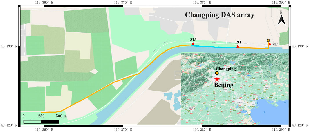
FIGURE 1. DAS array in Changping, Beijing. The yellow line is the optical cable, and the yellow circle indicates the location of the DAS interrogator. We used data from the sub-array (No. 191–315, blue line) and No. 91 (one of the cross-road channels) for traffic monitoring.

On the riverbank is a road that serves as the primary transportation artery for the nearby residents. The passing vehicles on the road would cause vibrations and generate seismic waves that will propagate to nearby optical cables and generate cable strain deformations. These deformations will be densely recorded by the DAS array, and the movement of every vehicle appears as a trajectory in DAS temporal–spatial recordings. According to the existence of the trajectory and its pattern, we can judge the passing vehicle, its speed, and the direction through traditional seismic array processing, image recognition, or even direct visual inspection.

We utilized about 500 m of fiber in the east (channels from 191 to 315, Figure 1) to monitor the traffic flow. This section of the fiber is roughly parallel to the road but about 20 m apart (Figure 1). In addition, the eastern portion contains a piece of cable (channel 91) that spans the road and allows a direct measurement of the vehicle-caused road vibration. The flows at the east and west may be different since some vehicles may stop by a restaurant that is situated between channels 91 and 191. The overall processing flow is shown in Figure 2.

FIGURE 2

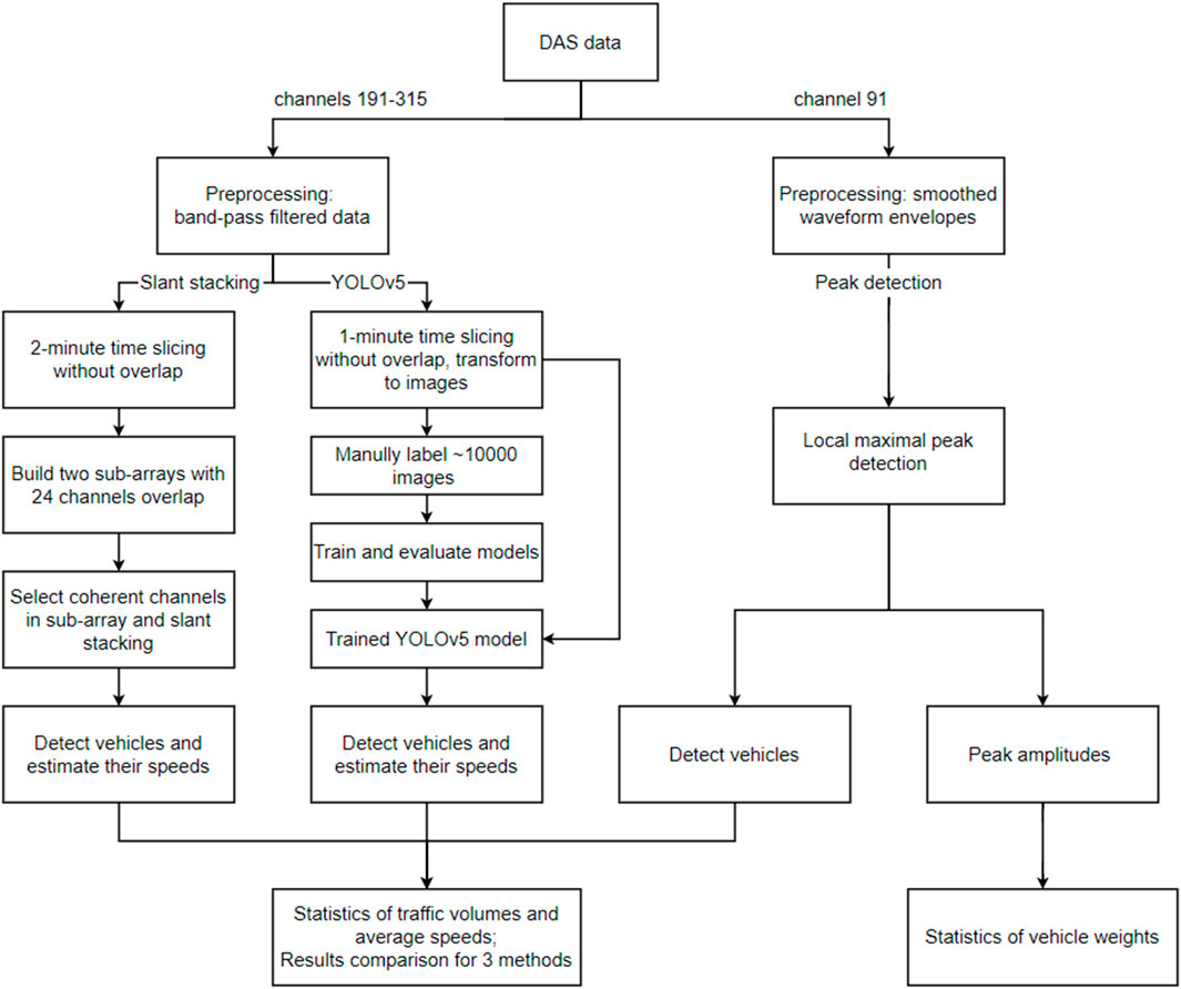
FIGURE 2. Overall data processing flow.

Distributed acoustic sensing data preprocessing

We first downsampled the continuous DAS data on channel 191–315 to 200 Hz and removed the linear trend, the mean value, and the common-mode noise. As the spectrum diagrams of two representative channels shown in Supplementary Figure S1, the background ambient noises are abundant at 1–20 Hz, while the vehicle signals above 20 Hz are easier to be separated from the background noises. On the other hand, vehicle signals below 1 Hz are only obvious for some heavy vehicles but not common for all; therefore, we apply a 20–50 Hz bandpass filter to the DAS data to improve the reliability of passing vehicle identification.

Passing vehicle detection and speed estimation with YOLOv5

YOLOv5 is the most recent version of the YOLO series (https://github.com/ultralytics/yolov5). One significant improvement is the detection speedup by PyTorch (Paszke et al., 2019), which can work with deeper networks for applications on more extensive datasets and real-time cases. The structure of YOLOv5 comprises four parts: the input, backbone network, neck network, and prediction network.

The principle of object detection is to use an anchor to select an image segment from the image and input it into the convolutional neural network model to identify the object category in the frame. By scanning the entire image with anchors of different sizes, we recognize and locate the object when the probability of the box-selected image segment predicted as ground truth is greater than the set threshold. The object detection algorithm is divided into two categories according to the processing steps. The two-stage method generates a series of region proposals through a particular module. It then uses a convolutional neural network for sample classification and regression positioning to detect objects represented by Faster R-CNN (Ren et al., 2015). The one-stage method directly extracts features from anchors to predict the object category and location, as described by SSD (Liu et al., 2016) and YOLO series (Redmon et al., 2016; Redmon and Farhadi, 2017; Redmon and Farhadi, 2018). Two-stage detection has high accuracy but slow detection speed. One-stage detection accuracy is low but much faster than the two-stage algorithm and is widely used in real-time object detection tasks.

We preprocessed DAS continuous waveforms for channels 191–315 into 1-min segments without overlap. The 1-min waveforms of 125 channels were converted to images in the size of 1167*875, resulting in around 21,000 photographs over the course of 15 days. To train a new YOLOv5 model for vehicle detection and speed estimation, we manually annotated a dataset of about 10,000 photographs.

For vehicle trace labeling in DAS images, LabelImg (2022) is employed. LabelImg is a graphical image annotation tool that labels object bounding boxes in images. These images are manually categorized as automobiles with varying speeds or noises without any car passing. First, we utilize bounding boxes for each image to entirely contain the vehicle traces with a predetermined size. One box represents an automobile that has been labeled, and the car number is the sum of the number of boxes. As the vehicle traces are contained within the boxes, the height and width of the boxes correspond to the driving distance and journey duration of the cars. Therefore, it is possible to determine the speed ranges of vehicles by calculating the aspect ratio of the bounding boxes. Once vehicle traces have been tagged, the width, height, and center coordinates of the boxes are automatically recorded as the ground-truth location for model training.

By counting the number of boxes and computing their box aspect ratio, we can determine the number of cars and their speed in each 1-min DAS image. In a ratio of 8:1:1, the dataset is randomly divided into training, validation, and testing sets. For training, we employ the SGD (Robbins and Monro, 1951) optimizer with momentum and weight decay coefficients of 0.937 and 0.0005, respectively. The learning rate is 0.01, and the initial training epoch has been set to 300. The deep learning processing flow of YOLOv5 is shown in Supplementary Figure S2. Due to the early stop mechanism, the training process on a server with two Nvidia GeForce RTX 3090 GPUs was terminated at epoch 228 after 10 h of training (Figure 3). Currently, the best model is the No. 128 epoch, with training precision as high as 95.9% (Figure 3).

FIGURE 3

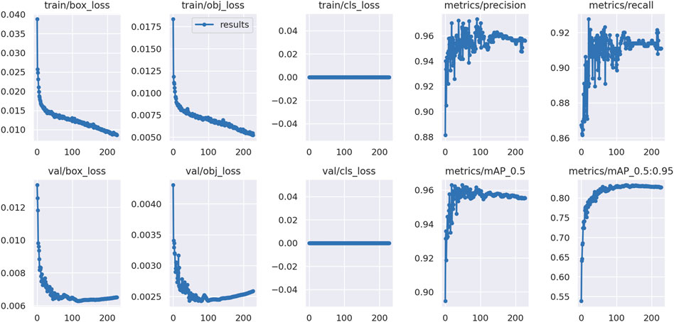
FIGURE 3. Vehicle detection YOLOv5 model training. Box regression loss (box loss), object loss (obj loss), class loss (cls loss), training accuracy, and recall are depicted in the top row, from the left to the right. Similar to the first row, the first three figures in the second row are loss functions for the validation set instead. The next two figures represent the mean average precision for IoU thresholds greater than 0.5 and for the range (0.5, 0.55, 0.60, ..., 0.95).

Box loss, object loss, and class loss are the primary evaluative factors for object detection algorithms. Given that the length and width of the boxes are critical to the distance and travel time of vehicle traces in DAS photographs, the box’s dimensions are crucial in this instance. The slight box loss provides a more precise bounding box position and enhances the speed estimation performance. YOLOv5’s box loss is a CIoU (complete intersection over union) loss between the predicted and ground-truth box (Zheng et al., 2020). IoU (intersection over union) is computed in the following manner:

$\begin{array}{c}IoU=\frac{\left|B\cap B^{gt}\right|}{\left|B\cup B^{gt}\right|}\end{array},(1)$

where B^gt = (x^gt, y^gt, w^gt, and h^gt) is the ground-truth bounding box and B = (x, y, w, and h) is the predicted bounding box.

CIoU loss is defined as follows:

$\begin{array}{c}{L}_{CIoU}=1-IoU+\frac{{\rho }^2\left(b,b^{gt}\right)}{c^2}+\alpha v\end{array},(2)$

where b and b^gt denote the central points of B and B^gt, ρ² represents the square of the distance between the center points of the prediction box b and the gt (ground-truth) box b^gt, and c² represents the square of the diagonal length of the smallest box that can just contain the prediction box and the gt box.

α as a trade-off parameter is shown in Eq. 3:

$\begin{array}{c}\alpha =\frac{v}{\left(1-IoU\right)+\nu }\end{array}.(3)$

Here, ν is used to measure the consistency of the aspect ratio between the predicted box and the gt box, and its definition is shown in Eq. 4:

$\begin{array}{c}v=\frac{4}{{\pi }^2}{\left(\mathit{arctan}\frac{w^{gt}}{h^{gt}}-\mathit{arctan}\frac{w}{h}\right)}^2\end{array},(4)$

where w^gt and h^gt, respectively, represent the width and height of the gt box, and w and h, respectively, represent the width and height of the prediction box.

CIoU loss takes three geometric properties into account, i.e., the overlap area, central point distance, and aspect ratio, and leads to a faster convergence and better performance. It is apparent in the first column of Figure 4 that the box regression loss dropped rapidly within 10–20 epochs. Object loss is the confidence loss of ground-truth and predicted bounding boxes for determining the probability of whether there are objects in the predicted bounding box. Object loss uses BCE loss (binary cross-entropy loss) in YOLOv5. BCE loss is defined in Eq. 5:

$\begin{array}{c}{L}_{BCE}=\{\begin{array}{c}-\mathit{log}\left(p\right)y=1,\\ -\mathit{log}\left(1-p\right)Otherwise,\end{array}\end{array}(5)$

where p is the probability of the predicted bounding box belonging to the gt box, y represents the value of the ground-truth bounding box, and the value range of y is {1, 0}.

FIGURE 4

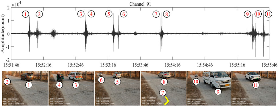
FIGURE 4. Cars across the cross-road fiber cable and their raw signals in the No. 91 DAS channel in the 4-min period. The cross-road fiber is beneath the white line in pictures. The events are labeled with numbers by time order. Cars No. 3 and No. 4 passed the channel almost the same time, and their waves are stacked together. Car No. 7 was not photographed since it turned to the restaurant as the yellow arrow indicates and did not have any signals captured on channels 191–315 during that time. Cars No. 2 and No. 4 also did not go through channels 191–315, according to our manual waveform inspection.

Class loss used in YOLOv5 is focal loss. Focal loss is defined as follows:

$\begin{array}{c}{L}_{focal}=-{\left(1-p_t\right)}^{\gamma }\mathit{log}\left(p_t\right)\end{array},(6)$

where p_t is the probability of the predicted class that belongs to the true class and γ is the focusing parameter (γ ≥ 0).

We only identified one class of automobile trace in the DAS photographs; hence, the class loss values of training and validation are both zero. There are considerable fluctuations in the first 100 epochs of the training precision and recall curves, but after the first 100 epochs, the curves gradually converge, and the accuracy is over 94%, and the recall is over 91%. In addition, the mean average accuracy with an IoU threshold of more than 0.5 is greater than 95%, and the mean average precision with an IoU threshold between 0.5 and 0.95 is close to 83%.

After training the model, we applied it to all DAS data and systematically recognized passing vehicles and their speed in the 15-day period. In a laptop with an Nvidia GeForce RTX 3060 Laptop GPU, the detection procedure only takes a total of about 0.5 h.

Passing vehicle detection and speed estimation by slant stacking

We also applied the slant stacking approach developed by Wang et al. (2021) to detect the passing vehicle and its speed. Similar to previous YOLOv5 processing, we segmented the prepossessed continuous DAS time series from the same 125 channels (about 500 m, the blue line in Figure 1) at 2-min intervals. The longer interval instead of 1 min can provide a more stable estimation of vehicle speed but will be more time-consuming during the slant stacking procedure. We used 2-min intervals for accurate speed estimation and for speeding up the computation. The 125 channels were further divided into sub-arrays with 74 channels and overlapped by 24 channels (i.e., slide with 50 channels). In each sub-array, we first performed data quality control by deleting these channels with a cross-correlation coefficient with adjacent channels smaller than 0.5. We then stacked the waveforms in the sub-array with the fourth root method (Rost and Thomas, 2002) by scanning the different vehicle trace slopes (p). The vehicle’s speed(c) can be determined as follows:

$\begin{array}{c}c=\frac{m\ast s}{p\ast dt}\end{array},(7)$

where m, s, and dt are the number of channels, the channel interval, and the time sampling rate, respectively. In this study, the values are 125, 4 m, and 0.05 s, respectively. We have established a speed estimation range of over 25 km/h to 100 km/h based on road conditions. This indicates that the slope p ranges from 28.8 to 115.2 in one direction and −115.2 to −28.8 in the opposite direction. The sign of p conveys information about the movement direction.

We shifted both sides of the middle channel of each subarray’s p*dt samples in the opposite direction and then stacked their energies. In addition, we utilized local maxima analysis to identify the peaks in order to estimate the number of vehicles and their speeds per 2 min. The results of the two sub-arrays are mutually verified for reducing vehicle detection and speed estimation errors by calculating the mean values of the vehicle numbers and speed ranges, respectively. All of the aforementioned DAS data slant stack processing procedures require roughly 85 h serially running on a Linux server with two AMD EPYC 7702 64-Core processors.

Due to the proximity of the fiber cable to the road in comparison to the measurement length, both the apparent speeds determined by YOLOv5 and slant stacking are considered to be the vehicle speed. Using the following formula, we estimated the hourly average speed (v_avg) as follows:

$\begin{array}{c}{v}_{avg}=\frac{{\sum }_{i=1}^n{v}_i}{n}\end{array},(8)$

where v_i is the individual vehicle speed detected by YOLOv5 or the slant stacking method and n is the number of vehicles in 1 hour.

Detection of vehicles and analysis of their weights by waveform amplitudes

Using transient fluctuations in waveform energy (amplitude) is a conventional technique for detecting seismic events, and it can also be utilized to detect passing cars. This detection can be performed with a single sensor, which is simple and requires minimal computational resources. But the method is difficult to estimate the movement speed and is more likely to be falsely triggered by pedestrians or other non-vehicle vibrations in the vicinity.

The continuous waveforms in a piece of cross-road cable (channel 91 in Figure 1) were independently used to count the vehicle number. As shown in Figure 4, moving automobiles caused obvious waveform changes, and their amplitudes may be relative to the vehicle’s weight. The original waveforms in this channel were downsampled, detrended and mean value removed, then transformed to waveform envelopes and smoothed with 2-s windows.

We used local maximal analysis to detect the events. Through several tests, the amplitude threshold and minimum event interval are set to 2000 count and 2 s, respectively.

Results

Vehicle detection comparison and verification

We begin by comparing the detections of the three techniques. On channel 91, we use a 4-min window for peak detection (Figure 4). During this time, we took photographs of vehicles crossing the channel. Photographs and waveforms on the channel confirm the passage of 11 vehicles within a 4-min period. For slant stacking and YOLOv5 methods, we extend the 4-min window on channels 191–315 by 1 minute at both ends. Due to the distance between the two observation sites (approximately 400 m) and the time shifts caused by passing vehicles, the 6-min window will ensure that the measurements for the three methods overlap.

We visually inspect the DAS array records for 11 vehicles that passed channel 91 and confirm that three of them (No.2, 4, and 7 in Figure 5) did not enter channels 191–315. Therefore, the ground-truth passed vehicle numbers for channel 91 are 11 and those for the DAS array on channels 191–315 are 8. Table 1 shows the vehicle detection verification of peak detection, slant stacking, and YOLOv5 methods. The number detected by the peak method is 13, and the three incorrectly detected signals are likely the result of local vibrations, such as people walking or a stopped car with its engine running. Supplementary Figure S3 shows more similar wrong detection cases, implying that the single-channel detection approach is susceptible to both moving vehicles and local events. The slant stacking and YOLOv5 methods each identify seven and eight vehicles, respectively. The absence of a detected vehicle in slant stacking is primarily due to the fact that the event signals on the different channels are split by the time window, and the stacking energies in both windows are too weak to identify (Figure 5). Two cars (Nos. 10 and 11) that are following closely are correctly identified by either slant stacking or YOLOv5. Unlike the slant stacking, a trace across two windows may be detected twice by YOLOv5 (Figure 5), which needs to remove duplicates by comparing their speeds and corner coordinates at the adjacent boxes. Other strong vibrations on channels 191–315 that are unrelated to traffic can be efficiently suppressed using both array-based methods, as shown in Supplementary Figure S3.

FIGURE 5

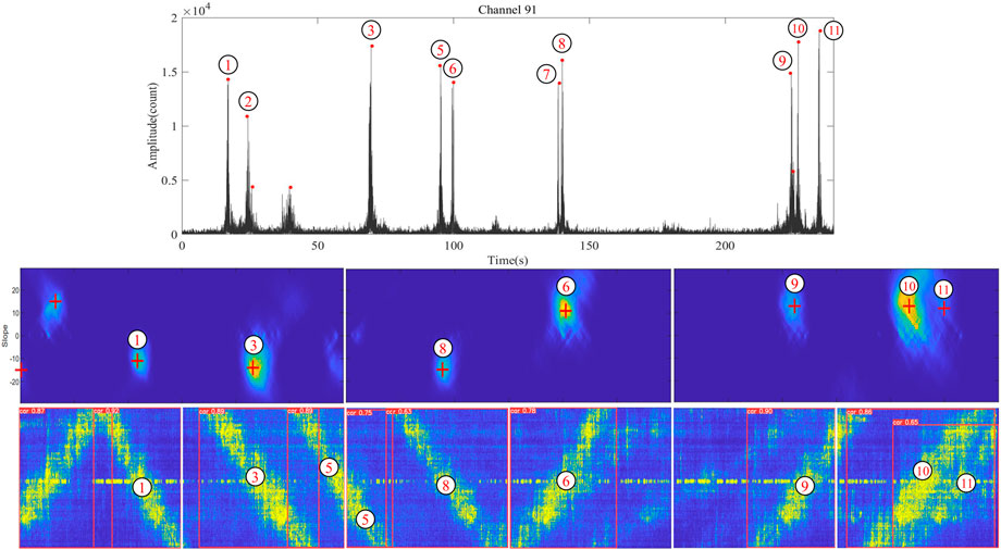
FIGURE 5. Vehicle detection comparisons. The three planes from up to down correspond to the findings of peak detection, slant stacking, and YOLOv5. Their respective detections are indicated by red dots, crosses, and boxes with correlation coefficients. The numbers in the circles are identical to those in Figure 4, but their order has altered due to their differing movement orientations. Cars 2, 4, and 7 do not pass through the DAS array on channels 191–315.

TABLE 1

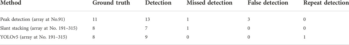
TABLE 1. Vehicle detection verification.

Traffic flow estimation and analysis

We used YOLOv5, slant stacking, and event peak detection to identify passing vehicles in about 2 weeks’ worth of DAS data between 11/12/2021 00:00 (Saturday) and 25/12/2021 20:00 (Monday) for the investigation of traffic patterns. We compared the variations in the number of automobiles per hour detected by the aforementioned three independent approaches. As seen in Figure 6, the three estimation methods for traffic volume yield comparable traffic patterns but differ in terms of the number of vehicles. The event peak detection method predicts the greatest number of vehicles, whilst the YOLOv5 method estimates a somewhat lower number, and the slant stacking method estimates the smallest number.

FIGURE 6

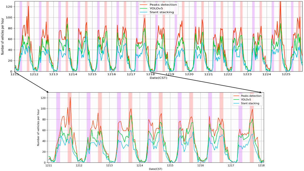
FIGURE 6. Daily variations in the traffic volume for event peak detection, YOLOv5, and slant stacking methods in 15 days. The zoom-in image in the lower panel highlights daily and weekly periodic patterns.

Traffic volume estimations are affected by a number of variables. One of the causes is the variance in the processing time window. With shorter time windows, more vehicles would be spotted, particularly during rush hour, but they would also be identified many times because the signals may span two units of data in continuous time series for array-based algorithms, such as YOLOv5 or slant stacking. False identifications can be avoided to a considerable extent with array-based approaches, which need coherent signals over many channels. In contrast, we discovered erroneous identifications in the peak detection method, where the erroneous peaks were likely generated by the neighboring tree swaying in windy conditions. In order to acquire more dependable traffic patterns, it is necessary to improve the detection algorithm, such as recognizing multiple objects simultaneously in an array-based approach.

Similar daily and weekly fluctuations exist for each of the three procedures. Each day’s traffic volume peaks in the morning, lowers during the midday, reaches another peak in the afternoon, and finally declines in the evening. We emphasize the two traffic volume peaks that occur within a certain time period for each technique, illustrating the weekday peaks. On weekdays, the morning rush hour occurs between 6 and 9 h, and the afternoon rush hour occurs between 15 and 18 h. However, this tendency is not appropriate on weekends, as depicted in the graph. From the zoomed-in graph, we can note that the weekday traffic volume peaks are quite narrow. We also find it intriguing that all methodologies forecast Friday’s morning rush hour to have significantly less traffic volume than other days. The weekly variations with a regular pattern may be related to the commute times of nearby neighbors.

We study the hourly traffic volume variations of event peak detection, YOLOv5, and the slant stacking method in greater detail (Figure 7). The majority of traffic volume accumulates between the morning and afternoon rush hours. During 6–18 h, the traffic volume of the event peak detection method ranges from 40 to 100 vehicles per hour, the YOLOv5 method ranges from 30 to 80 vehicles per hour, and the slant stacking method ranges from 20 to 60 vehicles per hour. The traffic volume estimation of the YOLOv5 approach is more accurate than that of the slant stacking method as the results of event peak detections represent the actual traffic volume. The hourly variance of each day is divided into five time-groups based on the morning and afternoon rush hours. From 0 to 6 h is the initial time where the majority of traffic volume is less than 10 vehicles per hour. The morning rush hour is the second interval between 6 and 9 a.m. Compared to 9–15 h, the third session has a relatively lower but stable volume of traffic. The afternoon rush hour is the fourth time between 15 and 18, characterized by the biggest volume of traffic. The final phase, between 18 and 0 h, is characterized by a sharp decline in the traffic volume.

FIGURE 7

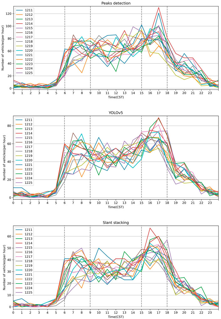
FIGURE 7. Hourly traffic volumes of 15 days derived from three detection methods. Different colored lines correspond to each day, and the gray vertical dot lines represent the rush hour.

Vehicle speed estimation

Figure 8 depicts the average speed variation of YOLOv5 and slant stacking. The YOLOv5 mean speed ranges between 30 km/h and 80 km/h, while the slant stacking method ranges between 30 km/h and 90 km/h. In general, the mean speed predicted by the slant stacking method is around 10 km per hour faster than YOLOv5. A vehicle trace in a DAS image is a width-measured line (the last panel in Figure 5). The slope of the middle section of the line is more representative of the actual vehicle speed. When the bounding box identified by YOLOv5 entirely encloses the entire vehicle trail, the speed calculated by the aspect ratio of the bounding box is always lower. The speed determined via slant stacking is more accurate than that of YOLOv5. The YOLOv5 technique speed range is upward and rises from 40 km/h to 60 km/h, whereas the slant stacking method speed range rises from 50 km/h to 70 km/h during the day. Figure 8’s top row depicts the daily and weekly fluctuations of the average speed assessed using YOLOv5 and the slant stacking approach. The fluctuations in the average speed over time for YOLOv5 and slant stacking are comparable. During the interval between midnight and dawn, the average speed of both the techniques is very variable, and the period contains both the minimum and maximum average speeds. In the second row of Figure 8, both the methods exhibit a gradual decrease in the average speed from six to eighteen o’clock, which corresponds to the rush hour periods discussed in the previous section. The average speed decreases from 60 km/h to 50 km/h for the YOLOv5 method and from 70 km/h to 50 km/h for the slant stacking method.

FIGURE 8

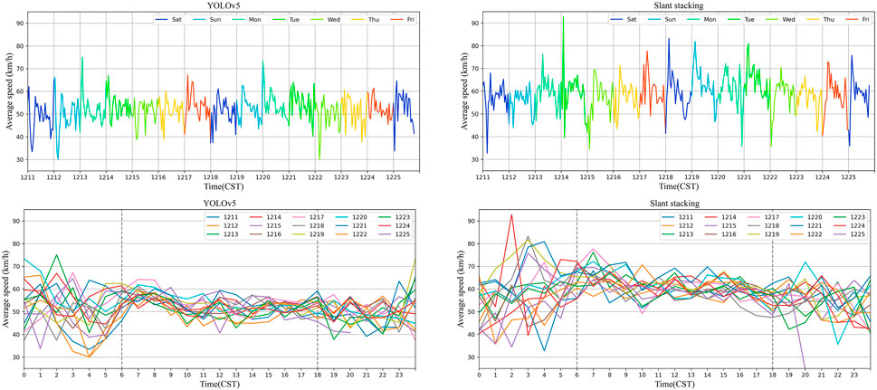
FIGURE 8. Figures in the top row represent the daily and weekly variations of the average speed, as estimated by YOLOv5 and the slant stacking technique. The figures in the second row represent hourly variations of the same methods. The gray dot line in the second row of figures divides each day into three distinct time intervals with varying average speed trends.

On the graphs of the hourly traffic volume and mean speed, we compare the results of YOLOv5 and the slant stacking method (Figure 9). For YOLOv5, there are less vehicles between midnight and early morning with divergent average speeds between 30 km/h and 80 km/h, while the majority of the vehicles are concentrated during the day with convergent average speeds between 40 km/h and 60 km/h. Slant stacking demonstrates the same distribution as YOLOv5 but with greater mean speeds and smaller traffic volume; the midnight and early morning period mean speed range is over 30–90 km/h, and the daylight period mean speed range is over 50–70 km/h.

FIGURE 9

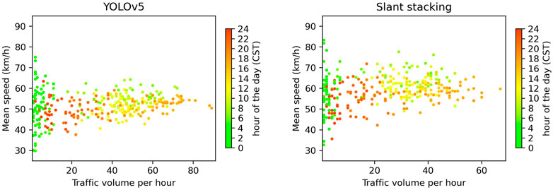
FIGURE 9. Relationship between the traffic volume and mean speed derived from the detection results of YOLOv5 (left) and slant stacking (right). The colors of the scatters represent the time of the day.

Vehicles classified by amplitude

The DAS-measured vehicle-passing amplitude is roughly proportional to the vehicle’s mass and load. In general, the stronger the vibration, the greater the total mass is. Figure 10 depicts the distribution of amplitudes across time for all identified events, while Figure 11 compares the vehicle numbers and their average amplitudes during the daily hours. Similar distributions are seen to those depicted in Figure 9. On the basis of these distributions, we broadly split the amplitudes into three categories: amplitudes higher than 12,500 counts, amplitudes fewer than 5,000 counts, and amplitudes in between. Figure 12 shows the vehicle counts over time for the three groups and their respective totals, binned per hour. Similar time-distribution features exist across the medium-amplitude bins and the entire event volume. Generally, the high-amplitude and low-amplitude distributions exhibit contrasting characteristics. High-amplitude gears usually appear during the morning rush hour, whereas low-amplitude values typically appear during the evening rush hour. These periods include high and low vehicle speeds, respectively (Figure 8). Figure 8 depicts that the average hourly velocity variation during the morning rush is greater than that of the evening rush, which is consistent with the high and low amplitudes depicted in Figure 12. Consequently, we hypothesize that the vehicle speed can influence the amplitude. Also, there is a link between velocity and amplitude; the faster the velocity, the greater the amplitude is.

FIGURE 10

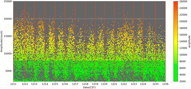
FIGURE 10. Passing vehicles’ amplitudes over the time.

FIGURE 11

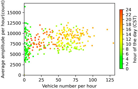
FIGURE 11. Hourly vehicle numbers and their mean amplitudes from peak detection. The colors of scatters represent the hour of the day.

FIGURE 12

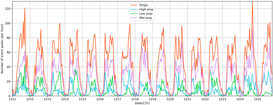
FIGURE 12. Distributions of vehicle numbers per hour for different vehicle weights. The vehicles are categorized into three classes: amplitude over 12,500 counts (High amp), lower than 5,000 counts (Low amp), and between 5,000 and 12,500 counts (Middle amp). The origin line is for total numbers.

Conclusion

In this study, we present a deep learning strategy based on the YOLOv5 real-time object recognition framework for recognizing the passage and velocity of automobiles in DAS photographs. After training on a massive amount of labeled data, our model’s precision is 95.9%. The new strategy for vehicle detection and speed estimation yields comparable results to the conventional slant stacking seismic array processing method. Unlike slant stacking, its processing speed for processing large DAS data is significantly faster, and it can be implemented in near-real-time data processing situations. With rapid data processing capacity, constructing a city-wide DAS network for traffic monitoring will be viable and operable using the city’s existing densely packed communication optical fiber network. In addition to augmenting the existing traffic video surveillance network, the network will also help for the development of smart cities.

Traditional seismic array processing, such as slant stacking, can use wavefield attributes to reconstruct vehicle motion parameters, such as driving directions, and is immediately applicable in a number of contexts. Deep learning requires the training of pertinent models. Because we did not identify the driving direction to construct a comparable training set, the system cannot discern the driving direction of the car in this experiment. Currently, we lack more comprehensive training for difficult situations, such as multiple vehicles passing simultaneously. This area must be expanded in the near future. In addition, the model’s ability to generalize across diverse circumstances has not been fully evaluated. In addition, integrating YOLOv5 with the slant stacking technique may help calibrate YOLOv5’s speed estimation and improve the performance of the YOLOv5 algorithm.

Copyright ^© 2022 Ye, Wang, Wang, Yang, Peng, Yan, Kou, and Yuan. This is an open-access article distributed under the terms of the Creative Commons Attribution License (CC BY). The use, distribution, or reproduction in other forums is permitted, provided the original author(s) and the copyright owner(s) are credited and that the original publication in this journal is cited, in accordance with accepted academic practice. No use, distribution, or reproduction is permitted which does not comply with these terms.

Data availability statement

The original contributions presented in the study are included in the article/Supplementary Material; further inquiries can be directed to the corresponding author.

Author contributions

ZY and WW conceived the main ideas, led the project, and wrote the initial draft of the manuscript. XW provided the code of the slant stacking method. All authors reviewed the results and contributed to the writing of the final manuscript.

Funding

This work was supported by the Project of Basic Scientific Research Foundation of Institute of Earthquake Forecasting, China Earthquake Administration (Grant Nos. CEAIEF20220402 and 2020IEF0602) and the National Natural Science Foundation of China (Grant Nos. 41574050 and 41674058) and was also supported by the Young Elite Scientists Sponsorship Program by CAST (grant 2020QNRC001), and the Key Research Program of the Institute of Geology & Geophysics, CAS (grant IGGCAS-201904).

Acknowledgments

The authors thank the editor YW and two reviewers HQ and SY for their constructive comments.

Conflict of interest

The authors declare that the research was conducted in the absence of any commercial or financial relationships that could be construed as a potential conflict of interest.

Publisher’s note

All claims expressed in this article are solely those of the authors and do not necessarily represent those of their affiliated organizations, or those of the publisher, the editors, and the reviewers. Any product that may be evaluated in this article, or claim that may be made by its manufacturer, is not guaranteed or endorsed by the publisher.

Supplementary material

The Supplementary Material for this article can be found online at: https://www.frontiersin.org/articles/10.3389/feart.2022.992571/full#supplementary-material

References

Al-qaness, M. A. A., Abbasi, A. A., Fan, H., Ibrahim, R. A., Alsamhi, S. H., and Hawbani, A. (2021). An improved YOLO-based road traffic monitoring system. Computing 103 (2), 211–230. doi:10.1007/s00607-020-00869-8

CrossRef Full Text | Google Scholar

Amitha, I. C., and Narayanan, N. K. (2021). “Object detection using YOLO framework for intelligent traffic monitoring,” in Machine vision and augmented intelligence—theory and applications. Editors M. K. Bajpai, K. Kumar Singh, and G. Giakos (Singapore: Springer), 405–412. doi:10.1007/978-981-16-5078-9_34

CrossRef Full Text | Google Scholar

Cao, C.-Y., Zheng, J.-C., Huang, Y.-Q., Liu, J., and Yang, C.-F. (2019). Investigation of a promoted you only look once algorithm and its application in traffic flow monitoring. Appl. Sci. 9 (17), 3619. doi:10.3390/app9173619

CrossRef Full Text | Google Scholar

Chambers, K. (2020). Using DAS to investigate traffic patterns at Brady Hot Springs, Nevada, USA. Lead. Edge 39 (11), 819–827. doi:10.1190/tle39110819.1

CrossRef Full Text | Google Scholar

Ge, L., Dan, D., and Li, H. (2020). An accurate and robust monitoring method of full-bridge traffic load distribution based on YOLO-v3 machine vision. Struct. Control Health Monit. 27 (12), e2636. doi:10.1002/stc.2636

CrossRef Full Text | Google Scholar

LabelImg (2022). heartexlabs. Available at: https://github.com/heartexlabs/labelImg (Accessed August 10, 2022).

Google Scholar

Lin, C.-J., and Jhang, J.-Y. (2022). Intelligent traffic-monitoring system based on YOLO and convolutional fuzzy neural networks. IEEE Access 10, 14120–14133. doi:10.1109/ACCESS.2022.3147866

CrossRef Full Text | Google Scholar

Lindsey, N. J., Yuan, S., Lellouch, A., Gualtieri, L., Lecocq, T., and Biondi, B. (2020). City-scale dark fiber DAS measurements of infrastructure use during the COVID-19 pandemic. Geophys. Res. Lett. 47 (16), e2020GL089931. doi:10.1029/2020gl089931

PubMed Abstract | CrossRef Full Text | Google Scholar

Liu, H., Ma, J., Xu, T., Yan, W., Ma, L., and Zhang, X. (2019). Vehicle detection and classification using distributed fiber optic acoustic sensing. IEEE Trans. Veh. Technol. 69 (2), 1363–1374. doi:10.1109/tvt.2019.2962334

CrossRef Full Text | Google Scholar

Liu, W., Anguelov, D., Erhan, D., Szegedy, C., Reed, S., Fu, C. Y., et al. (2016). “Ssd: Single shot multibox detector,” in European conference on computer vision (Cham: Springer), 21–37.

CrossRef Full Text | Google Scholar

Mandal, V., Mussah, A. R., Jin, P., and Adu-Gyamfi, Y. (2020). Artificial intelligence-enabled traffic monitoring system. Sustainability 12 (21), 9177. doi:10.3390/su12219177

CrossRef Full Text | Google Scholar

Narisetty, C., Hino, T., Huang, M. F., Ueda, R., Sakurai, H., Tanaka, A., et al. (2021). Overcoming challenges of distributed fiber-optic sensing for highway traffic monitoring. Transp. Res. Rec. 2675 (2), 233–242. doi:10.1177/0361198120960134

CrossRef Full Text | Google Scholar

Paszke, A., Gross, S., Massa, F., Lerer, A., Bradbury, J., Chanan, G., et al. (2019). Pytorch: An imperative style, high-performance deep learning library. Adv. neural Inf. Process. Syst. 32.

Google Scholar

Redmon, J., Divvala, S., Girshick, R., and Farhadi, A. (2016). “You only look once: Unified, real-time object detection,” in Proceedings of the IEEE conference on computer vision and pattern recognition, 779–788.

CrossRef Full Text | Google Scholar

Redmon, J., and Farhadi, A. (2017). “YOLO9000: Better, faster, stronger,” in Proceedings of the IEEE conference on computer vision and pattern recognition, 7263–7271.

CrossRef Full Text | Google Scholar

Redmon, J., and Farhadi, A. (2018). Yolov3: An incremental improvement. arXiv preprint arXiv:1804.02767.

Google Scholar

Ren, S., He, K., Girshick, R., and Sun, J. (2015). Faster r-cnn: Towards real-time object detection with region proposal networks. Adv. neural Inf. Process. Syst. 28.

Google Scholar

Robbins, H., and Monro, S. (1951). A stochastic approximation method. The annals of mathematical statistics, 400–407.

CrossRef Full Text | Google Scholar

Rost, S., and Thomas, C. (2002). Array seismology: Methods and applications. Rev. Geophys. 40 (3), 2-1–2-27. doi:10.1029/2000rg000100

CrossRef Full Text | Google Scholar

Stork, A. L., Baird, A. F., Horne, S. A., Naldrett, G., Lapins, S., Kendall, J.-M., et al. (2020). Application of machine learning to microseismic event detection in distributed acoustic sensing data. GEOPHYSICS 85 (5), KS149–KS160. doi:10.1190/geo2019-0774.1

CrossRef Full Text | Google Scholar

van den Ende, M. P. A., Ferrari, A., Anthony, S., and Richard, C. (2021). Deep deconvolution for traffic analysis with distributed acoustic sensing data. hal-03352810.

Google Scholar

Wang, X., Williams, E. F., Karrenbach, M., Herraez, M. G., Martins, H. F., and Zhan, Z. (2020). Rose parade seismology: Signatures of floats and bands on optical fiber. Seismol. Res. Lett. 91 (4), 2395–2398. doi:10.1785/0220200091

CrossRef Full Text | Google Scholar

Wang, X., Zhan, Z., Williams, E. F., Herráez, M. G., Martins, H. F., and Karrenbach, M. (2021). Ground vibrations recorded by fiber-optic cables reveal traffic response to COVID-19 lockdown measures in Pasadena, California. Commun. Earth Environ. 2 (1), 160–169. doi:10.1038/s43247-021-00234-3

CrossRef Full Text | Google Scholar

Wiesmeyr, C., Coronel, C., Litzenberger, M., Döller, H. J., Schweiger, H. B., and Calbris, G. (2021). “Distributed acoustic sensing for vehicle speed and traffic flow estimation,” in 2021 IEEE international intelligent transportation systems conference (ITSC) (IEEE), 2596–2601.

CrossRef Full Text | Google Scholar

YOLO (2022). Real-time object detection. Available at: https://pjreddie.com/darknet/yolo/ (Accessed July 10, 2022).

Google Scholar

YOLOv5 framwork (2022). GitHub ultralytics. Available at: https://github.com/ultralytics/yolov5 (Accessed July 10, 2022).

Google Scholar

Zheng, Y., Li, X., Xu, L., and Wen, N. (2022). A deep learning–based approach for moving vehicle counting and short-term traffic prediction from video images. Front. Environ. Sci. 10. doi:10.3389/fenvs.2022.905443

CrossRef Full Text | Google Scholar

Zheng, Z., Wang, P., Liu, W., Li, J., Ye, R., and Ren, D. (2020). Distance-IoU loss: Faster and better learning for bounding box regression. Proc. AAAI Conf. Artif. Intell. 34 (07), 12993–13000. doi:10.1609/aaai.v34i07.6999

CrossRef Full Text | Google Scholar

Zhu, X., and Shragge, J. (2022). Toward real-time microseismic event detection using the YOLOv3 algorithm. Retrieved from https://eartharxiv.org/repository/view/2926/.

Google Scholar