A revised method with a temperature constraint for assimilating satellite-derived humidity in forecasting sea fog over the Yellow Sea

Numerical forecast of sea fog is very challenging work because of its high sensitivity to model initial conditions. For better depicting the humidity structure of the marine atmospheric boundary layer (MABL), Wang et al. (2014) assimilated satellite-derived humidity from sea fog at its initial stage over the Yellow Sea (W14 method), using an extended three-dimensional variational data assimilation (3DVAR) with the Weather Research and Forecasting model (WRF). This article proposes a revised version of the W14 method. The major ingredient of the revision is the inclusion of a temperature constraint into the satellite-derived humidity, not only for the missed fog area that the W14 method primarily considers, but also for the false fog area that is not handled in the W14 method. The numerical experiment results of 10 sea fog cases over the Yellow Sea show that the revised method can effectively alleviate the wet bias occasionally occurring in the W14 method, resulting in an improvement by about 15% for an equitable threat score of the simulated fog area. In addition, a detailed case study is conducted to illustrate the working mechanism of the revised method, including sensitivity experiments focusing on the roles of two kinds of background error covariances (CV5 and CV6) in the assimilation by the WRF-3DVAR. The results suggest that CV6 with multivariate cross-correlation is probably more beneficial to the revised method’s performance.

1 Introduction

Sea fog refers to the fog that occurs over seas or coastal areas with the atmospheric horizontal visibility less than 1 km, threatening the safety of marine transportation and activities and causing heavy casualties and property losses (Wang, 1985; Gultepe et al., 2007). Most sea fogs belong to the advective cooling type, such as the sea fog over the Yellow Sea (Wang, 1985; Gao et al., 2007). Its formation mechanism is that warm-moist air mass flows over the cold sea surface and gradually cools down to the dew point, which usually occurs over the regions with a strong sea surface temperature (SST) gradient located north of a warm current (Lewis et al., 2003). The Yellow Sea is such a region, with the Kuroshio warm current in the south (Figure 1). It experiences frequent fog events with an average of ∼50 fog days observed at its west coast, and its fog season starts in April and abruptly ends in August (Zhang et al., 2009; Fu et al., 2012). There are several major ports around the Yellow Sea, such as Qingdao, Dalian, Lianyungang, and Incheon. The busy international marine freight and traffic make it urgent to improve the forecasting skill of the sea fog over the Yellow Sea.

FIGURE 1

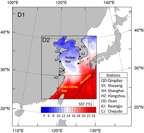
FIGURE 1. The Weather Research and Forecasting (WRF) model domain and the sites of radiosonde observations. Color shades denote the SST of the inner domain D2 on 28 April, 2008, and the thick line indicates the Kuroshio warm current.

With the rapid improvement of numerical models and computing power, numerical modeling has already been an important approach for sea fog research and forecast (Koračin and Dorman 2017). However, there are still some challenges in the numerical simulation of sea fog, one of which is the initial condition problem. Many studies have indicated that a sea fog simulation is very sensitive to the initial condition (Lorenz, 1965; Nicholls, 1984; Findlater et al., 1989; Ballard et al., 1991; Koračin et al., 2001; Lewis et al., 2003; Koračin et al., 2005a; Koračin et al., 2005b; Gao et al., 2007; Gao et al., 2010). The dominant synoptic system responsible for sea fog over the Yellow Sea is usually an isolated anticyclone, a cyclone–anticyclone couplet system, or a high-pressure ridge (Wang 1985; Zhou et al., 2004), which generally drives warm-moist air mass to continuously flow northward from the warmer sea area at low latitudes to the colder Yellow Sea. Due to the cooling by the cold sea surface, the thermal structure of the marine atmospheric boundary layer (MABL) over the Yellow Sea changes, resulting in the formation of sea fog (Gao et al., 2007; Yang and Gao 2015, 2020; Kim et al., 2021). Therefore, the initial conditions for sea fog simulation focus on the temperature and humidity structure of MABL (Gao et al., 2010). However, it is difficult to depict the accurate temperature and humidity structure of MABL, particularly for humidity, due to the coarse resolution of the background from global analysis and the rarity of marine observations.

Aware of the importance of the initial MABL structure for sea fog simulation, many studies have been carried out on sea fog data assimilation, which can be roughly divided into two aspects: the assimilation of unconventional observation data (Liu et al., 2011; Li et al., 2012; Wang and Gao, 2016; Wu et al., 2017; Gao and Gao 2019) and the exploration of data assimilation methods (Gao et al., 2010; Wang et al., 2014; Gao et al., 2018; Yang et al., 2021). The initial MABL structure benefits little from the direct assimilation of satellite radiance data (Li et al., 2012) due to the coarse resolution in the lower troposphere of the radiance data. The assimilation of QuickSCAT sea surface wind and Doppler radar radial wind can make the sea fog simulation better because the wind component of the initial MABL structure is improved (Liu et al., 2011; Wang and Gao 2016). However, the precondition for this improvement is that the temperature and humidity structure of MABL is appropriate. Compared with 3DVAR (three-dimensional variational) assimilation with static background error covariance, EnKF (ensemble Kalman filter) can produce a higher quality initial condition for sea fog simulation when assimilating the same observations (Gao et al., 2018) because it uses a dynamic flow-dependent background error covariance that can improve humidity from assimilating temperature. These previous studies have noted that the failure of sea fog modeling is usually caused by the error of MABL humidity in the initial condition. There is usually a dry bias within the MABL, which is not conducive to the formation of sea fog.

In order to correct the dry bias of humidity, Wang et al. (2014) proposed a method for assimilating satellite-derived humidity (hereafter denoted by the W14 method; see Section 2.1 for a brief review). In the W14 method, the satellite-derived humidity (i.e., 100% relative humidity in the three-dimensional space of sea fog occurrence) is first retrieved from the multifunctional transport satellite (MTSAT) of Japan, and then assimilated by an extended cycling 3DVAR based on the Weather Research and Forecasting (WRF) model. Two sea fog cases, one which spreads widely over the Yellow Sea and the other which spreads narrowly along the coast, were studied in detail for analyzing the feasibility of the W14 method. Additionally, the W14 method was applied on extra 10 sea fog cases to evaluate the effect of the W14 method. The assimilation of satellite-derived humidity can improve the equitable threat score (ETS) of the forecasted sea fog area by about 15% for the widespread-fog case, while the WRF model completely fails to reproduce the sea fog event without the assimilation of satellite-derived humidity for the narrowly spread coastal case. Additionally, the W14 method was applied on extra 10 sea fog cases for evaluation, and the result showed that ETS was improved by nearly 72% on average.

However, Wang et al. (2014) pointed out that the dry bias was over-corrected in some sea fog cases, that is, humidity increased excessively in the assimilation of satellite-derived humidity by using the W14 method, resulting in a large wet bias and sequentially over-forecasting fog area. In the W14 method, the satellite-derived humidity is relative humidity (RH), and it has to be converted into specific humidity (Qv; an acceptable variable in the WRF-3DVAR). During the conversion, pressure and temperature are needed, and they are extracted from the background analysis in the 3DVAR where sea fog might not exist and the temperature is higher than the SST. For a typical advection sea fog over the Yellow Sea, the temperature profile is near neutral once the sea fog grows up to some extent (Gao et al., 2007), indicating that the temperature within the sea fog is near the SST. This means that the given temperature during the conversion of RH to Qv in the W14 method is overestimated, resulting in Qv being overestimated because warmer air is able to hold more water vapor. This is most likely the reason why a large wet bias is produced by the W14 method in some sea fog cases.

The purpose of this study is to propose a revised version based on the W14 method (called revised method) to improve the W14 method to correct its false wet bias by adding temperature constraints, which is based on the existing mechanism research on sea fog over the Yellow Sea (Wang, 1985; Gao et al., 2007; Yang and Gao, 2020). The remaining article is organized as follows. Section 2 introduces the W14 method briefly, and describes the proposal of improving the W14 method. In Section 3, numerical experiments on 10 sea fog cases over the Yellow Sea are conducted, including data, model configuration, and experimental design. The evaluation of the data assimilation effect by using the revised method is implemented in Section 4. In addition, Section 5 studies a case in detail to analyze the impact of the temperature constraint added in the W14 method. Finally, a summary is given in Section 6.

2 Assimilation method

2.1 Brief review of the W14 method

The W14 method aims at the operational forecast of the sea fog over the Yellow Sea (Wang et al., 2014). Its idea is that if part of the sea fog has been formed in the assimilation window of the forecast, its three-dimensional space (3D-Space) can be obtained by satellite inversion. Assuming that the RH of the fog patch is 100%, then 3DVAR assimilation of the RH is conducted to improve the initial condition of sea fog forecast.

Based on previous studies (Ellrod 1995; Heidinger and Stephens, 2000; Bendix et al., 2005; Liu and Hu, 2008; Gao et al., 2009; Fu et al., 2011), Wang et al. (2014) developed a detection algorithm for sea fog over the Yellow Sea to obtain its 3D space using geostationary satellite data, including horizontal area and thickness (see details in the Section 2 of their article). The 3D-space is discretized into numerous humidity profiles with given horizontal and vertical grid intervals (ΔX and ΔZ). Since the air in the fog is saturated or nearly saturated (Sorli et al., 2002; Kim and Yum, 2010), the RH within the fog layers is assumed to be 100%. In Figure 2A, the schematic diagram of this discretization is demonstrated, and the thick dashed line shows a humidity profile with the variables P (pressure), T (temperature), Z (height), and RH with a value of 100%. Thereafter, the humidity profile is denoted by the sea fog humidity sounding. The value of Z is determined from the retrieval algorithm for sea fog with ΔZ. However, P and T have to be extracted from the analysis in the WRF-3DVAR.

FIGURE 2

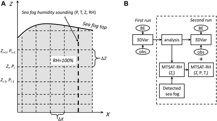
FIGURE 2. Schematic diagram for the two major ingredients of the W14 method: (A) sampling extraction of sea fog humidity sounding (i.e., MTSAT-RH) from the discretization of the observed fog area and (B) extension of one WRF-3DVAR update from running once to running twice for providing the MTSAT-RH with P (pressure) and T (temperature) from the analysis of the first run and then assimilating the MTSAT-RH. See the text for details.

The extended cycling 3DVAR scheme used in the W14 method is based on the work by Gao et al. (2010). The entire 3DVAR assimilation process sequentially consists of several 3DVAR updates in the assimilation window, among which Wang et al. (2014) extend a 3DVAR update from one run to two runs. Figure 2B shows this extension marked by a dashed frame. In Figure 2B, OBS represents routine observations (surface measurements and radiosondes) and a few satellite-retrieved temperature and humidity profiles, while MTSAT-RH refers to sea fog humidity soundings in Figure 2A. It can be seen that the analysis from the first 3DVAR run produces a background field for the second 3DVAR run, especially the required P (pressure) and T (temperature) information for MTSAT-RH.

2.2 Proposal of the revised method

For a typical advection fog over the Yellow Sea, there is a version layer in the MABL prior to fog formation (i.e., warm fog phase), and the inversion layer gradually deforms into a neutral stratification due to the sea surface cooling (Lewis et al., 2003; Gao et al., 2007). With the increase of sea fog thickness, the long-wave radiation cooling at the fog top results in top-down turbulence mixing (Koračin et al., 2014; Yang and Gao, 2020), causing the temperature in the fog to fall lower than SST (i.e., cold fog phase). The warm and cold fog phases are often observed (Kim and Yum, 2012; Huang et al., 2015; Yang et al., 2018; Yang and Gao, 2020). The physics process of sea fog evolution shows that the temperature profiles inside and outside sea fog are obviously different.

As mentioned in the introduction, in some sea fog cases, the W14 method over-corrected the dry bias of the MABL moisture status and even caused a large wet bias, resulting in the forecast of a false sea fog. According to the assimilation scheme of MTSAT-RH in Figure 2B, we infer that this is due to the use of incorrect temperature information in the assimilation. In the W14 method, the temperature given to MTSAT-RH (humidity sounding in Figure 2A) is extracted from the analysis of the first 3DVAR run. If the analysis has no sea fog in the detected fog layers, the given temperature is not consistent with sea fog physics. This is a defect of the W14 method. In addition, there is another defect. The method only detects humidity according to the detected sea fog, regardless of the wrong humidity result from the false sea fog forecast in the DA window. Therefore, we improve the W14 method here, adding a reasonable temperature constraint to make the assimilation of MTSAT-RH physically coordinated. Furthermore, we also deal with the false fog area generated in assimilation process.

Figure 3A shows a comparison diagram of the observed sea fog and simulated sea fog in the analysis produced by the first 3DVAR run (Figure 2B). The observed sea fog is the sea fog detected by the detection algorithm in the W14 method, while the simulated sea fog is defined by the areas where the simulated cloud–water mixing ratio is ≥0.016 g kg⁻¹ and the fog height is limited ≤400 m (Gao et al., 2010; Zhou and Du, 2010; Wang et al., 2014). In Figure 2B, “hit” denotes the area where both the observed sea fog and simulated sea fog exist, “false” denotes the area where the simulated sea fog exists but the observed sea fog does not, and “miss” denotes the area where the observed sea fog exists but the simulated sea fog does not (hereafter, these fog areas are called hit fog, false fog, and missed fog, respectively). The corresponding temperature profiles are also presented according to the previous research studies (Gao et al., 2007; Yang et al., 2018; Yang and Gao, 2020). The profiles T_c, T_f, T_h, and T_m indicate the temperature profiles within the areas of clear air, false fog, hit fog, and missed fog, respectively.

FIGURE 3

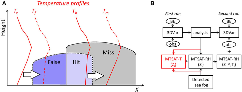
FIGURE 3. Schematic diagram of the revised method with the temperature constraint: (A) typical temperature profiles within the areas of clear air (T_c), false fog (T_f), hitting fog (T_h), and missed fog (T_m); (B) assimilation of sea fog humidity soundings in one 3DVAR update, including the temperature constraint (see the part marked in red color). See details in the text.

The focus to improve the W14 method is on the areas of missed fog and false fog, that is, adding a temperature constraint to these areas by the following operations:

$T_m\left(i_m,j_m,k_m\right)=SST\left(i_m,j_m\right)+\left[SAT\left(i_h,j_h\right)-SST\left(i_h,j_h\right)\right],(1)$

$T_f\left(i_f,j_f,k_f\right)=SST\left(i_f,j_f\right)+\left[T\left(i_c,j_c,k_f\right)-SST\left(i_c,j_c\right)\right](2)$

where $SAT$ is the simulated sea surface air temperature; i, j, and k represent model horizontal grid (i, j) and vertical grid (k), respectively; $\left(i_m,j_m,k_m\right)$ denotes a point within the missed fog area; and $\left(i_h,j_h\right)$ denotes the nearest point in the hit fog. $\left(i_f,j_f,k_f\right)$ denotes a point within the false fog area, and $\left(i_c,j_c\right)$ denotes the nearest point in the clear air area.

As seen from Eq. 1, within missed fog, $T_m$ is re-assigned based on SST and the air–sea temperature contrast within the hit fog area, and the profile is vertically homogeneous ($T_m$ does not vary with $k_m$; see Figure 3A). It can make the MABL of the missed fog area cooler and neutral, which is conducive to sea fog forming; whereas, within the false fog area, $T_f$ is replaced by a temperature profile with the vertical structure within the nearest clear air area (Eq. 2), which helps the dissipation of false fog because this clear-air temperature profile is warmer than that of the false fog area.

The aforementioned improvement process is modularized and inserted into the codes of the W14 method (see the part marked by red color in Figure 3B). Theoretically, the new method should be better than the original version because it considers the improvements of both missed fog and false fog areas. In the following sections, we carefully evaluate the revised method by numerical experiments on 10 sea fog cases over the Yellow Sea.

3 Numerical experiments

3.1 Data

The National Centers for Environmental Prediction (NCEP) Final Analysis (FNL) (1° × 1°; six hourly) provided initial and lateral boundary conditions for the simulation, and the SST data as the model bottom condition were derived from datasets of the North-East Asian Regional Global Ocean Observing System (NEAR-GOOS) (0.25° × 0.25°; daily).

Observations (i.e., obs in Figure 2B) used for assimilation in this study were downloaded from NCEP, including routine observations (surface, buoy, island measurements, and radiosondes), and some temperature and humidity profiles were retrieved from the atmospheric infra-red sounder (AIRS). Additionally, the detection algorithm for sea fog over the Yellow Sea used hourly albedo, infrared and visible cloud images of the MTSAT satellite.

Surface synoptic charts from the Korea Meteorological Administration (KMA) were used to show the weather situation involved with sea fog. The evaluation of the forecast using the precipitable water (PW; also called the columnar atmospheric water vapor) dataset (0.25° × 0.25°) was derived from satellite-bone microwave images, including the special sensor microwave imager (SSM/I), the special sensor microwave imager sounder (SSMIS), the advanced microwave scanning radiometer-E (AMSR-E), and the tropical rainfall measuring mission (TRMM) microwave imager (TMI). These satellite datasets were provided with quality control by remote sensing systems (RSS).

3.2 Model configuration

The advanced research core of the WRF with its WRFDA module (version 3.5.1; Skamarock et al., 2008) was employed for numerical experiments in this study. Two-way nesting was designed with the outer domain (D1; 30 km × 30 km) covering the northwest Pacific and most regions of East Asia and the inner domain (D2; 10 km × 10 km) over the entire Yellow Sea (Figure 1). Previous studies (Lu et al., 2014) have shown that the optimum combination of parameterizations for modeling of the Yellow Sea fog is the YSU PBL (Hong et al., 2006; Hong 2010) scheme and the Purdue Lin microphysics scheme (Lin et al., 1983);thus, YSU and Lin schemes were used in this study. The detailed model configurations were listed in Table 1.

TABLE 1

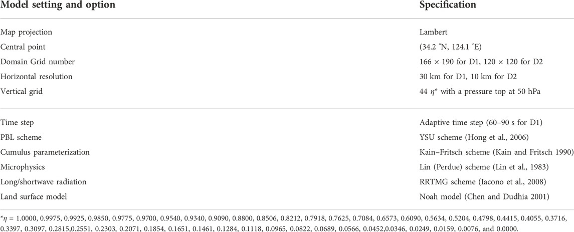
TABLE 1. WRF configuration.

The 3DVAR update used the default observation errors for assimilating different observations. The National Meteorology Center (NMC) method (Parrish and Derber, 1992) was adopted to generate a domain-dependent BE covariance for 3DVAR update. For each sea fog case, the WRF model was initialized every 12 h and ran 24 h for 15 days centered by the forecast initial time, and BE covariance was approximated by the average differences between 12-h and 24-h forecasts:

$\mathrm{B}\mathrm{E}\approx \overline{{(\mathbf{x}}^{12}–{\mathbf{x}}^{24}){{(\mathbf{x}}^{12}–{\mathbf{x}}^{24})}^{\mathrm{T}}},(3)$

where ${\mathbf{x}}^{12}$ and ${\mathbf{x}}^{24}$ are 12-h and 24-h forecasts, respectively. The control variables in BE include stream function, velocity potential, temperature, surface pressure, and pseudo-RH. Since the cross-correlations among control variables is important to sea fog modeling (Gao and Gao 2020), in the case study of Section 5, we compared the impacts of two kinds of BE covariances (CV5 and CV6) defined by the WRFDA module. The correlations between moisture (i.e., pseudo-RH) and other control variables exist in CV6, but not in CV5. These correlations might amplify the impact of temperature correction in the revised W14 method.

3.3 Experimental design

Three groups of numerical forecast experiments (hereafter called Group-A, Group-B, and Group-C) were designed and conducted for 10 sea fog cases. All the groups share the same model configuration listed in Table 1. All forecast experiments ran 24-h forecasts with 12-h data assimilation (DA) windows before the initial time (LST, =UTC+8). In the 12-h DA window, the 3DVAR update cycled five times with a DA interval of 3 h.

In Group-A, only obs was assimilated. Both obs and MTSAT-RH were assimilated in the other two groups. The DA in Group-B was treated with the W14 method, whereas Group-C was treated with the revised method. All the groups employed CV5 BE covariance, which is widely applied in operational forecast. Note that the ten cases and experimental design for Group-A and Group-B are the same as those in the article of Wang et al. (2014), except that the ARW version was changed from 3.3 to 3.5.1.

The purpose of the experiments is to show whether the temperature constraint (Group-C) can further improve the results, given that forecast with the W14 method (Group-B) is already quite successful. We are also concerned about whether the W14 method is still effective when updating the model version.

4 Numerical experiments

4.1 Evaluation method

The most important aspect of sea fog forecast is the horizontal fog area (abbreviated as fog area). The fog area detected by the detection algorithm in the W14 method is called the observed fog area, while the fog area diagnosed from the WRF hourly output is called the simulated fog area (see Section 2.1 for its diagnostic method). The observed and simulated fog areas are produced hourly, and their spatial resolution are 4 and 10 km, respectively.

To quantitatively evaluate the effects of the revised method, a series of prediction statistics were calculated for each experiment based on the comparison between simulated and observed fog areas (Zhou and Du, 2010). The inner domain (i.e., D2 in Figure 1) was taken as the evaluation domain, and its grid size was set to 0.1^o. Both fog areas were meshed onto the grids of the evaluation domain, and point-to-point comparisons were conducted. Note that both the land and sea areas covered by high-altitude clouds were excluded from the evaluation domain. The statistical scores include probability of detection (POD), false alarm ratio (FAR), bias score (BS), and equitable threat score (ETS), which are defined as

$\mathrm{P}\mathrm{O}\mathrm{D}=\frac{H}{O},(4)$

$\mathrm{F}\mathrm{A}\mathrm{R}=\frac{F-H}{F},(5)$

$\mathrm{B}\mathrm{S}=\frac{F}{O}(6)$

$\mathrm{E}\mathrm{T}\mathrm{S}=\frac{H-R}{F+O-H-R}(7)$

where H, F, and O denote the numbers of hit points, forecasted fogy points, and observed foggy points, respectively. R=F(O/N) is a random hit penalty, where N is the total number of grid points.

The radiosonde observations at seven coastal stations (shown in Figure 1) were used to evaluate the forecasted temperature and humidity profiles. Model results were interpolated to the pressure levels of the soundings, and the average bias and root-mean-square-error (RMSE) are calculated by

$\mathrm{b}\mathrm{i}\mathrm{a}\mathrm{s}=\frac{1}{n}{\displaystyle \sum }_{i=1}^n\left(x_i-y_i\right),(8)$

$\mathrm{R}\mathrm{M}\mathrm{S}\mathrm{E}=\sqrt{\frac{1}{n}{\displaystyle \sum }_{i=1}^n{\left(x_i-y_i\right)}^2},(9)$

where n is the number of stations, and $x_i$/$y_i$ is the forecasted/observed variable.

4.2 Effect analysis

The hourly simulated fog areas of the 10 sea fog cases were compared with the observed fog area. Table 2 shows the time averages of the statistical scores for all of the experiments.

TABLE 2

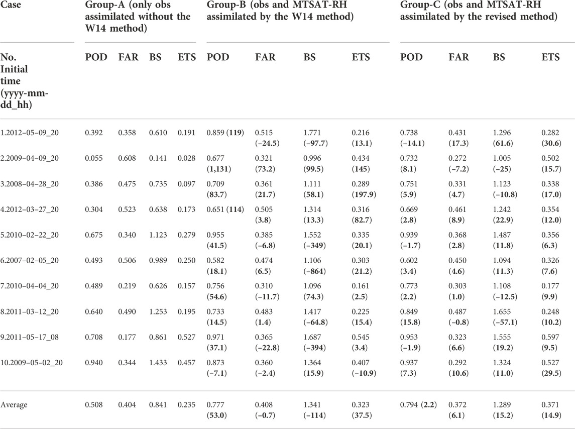
TABLE 2. Statistical scores for 10 cases. Bold numbers in parentheses for Group-B show the improvements (%) relative to Group-A, while those for Group-C show the improvements relative to Group-B.

It can be seen from Table 2 that the POD, FAR, BS, and ETS scores averaged over the 10 sea fog cases for Group-A which assimilate obs only are 0.508, 0.404, 0.841, and 0.235, respectively; by further assimilating MTSAT-RH using the W14 method, Group-B gets the scores of 0.777, 0.408, 1.341, and 0.323, respectively. This shows that the W14 method is effective, which improves POD and ETS by 53.0% and 37.5%, respectively. However, the BS increases for all cases, ranging from 0.834 to 1.341, indicating that the W14 method enlarges the simulated fog area. This helps greatly improve the situation where the sea fog forecast has almost failed (e.g., Case 2 and Case 3), but may reduce the situation where it is somewhat overestimated (e.g., Case 10). Note that for the same 10 cases, Wang et al. (2014) reported that the improvements of POD and ETS by using the W14 method are 60% and 70%, respectively. This study used the same experimental designs as them except using a newer version of the WRF model with an updated YSU scheme. The lower improvements here (53.0% and 37.5% for POD and ETS) are probably attributable to the revision of the YSU scheme. The turbulent diffusion within stable PBL is weakened in the YSU scheme of the WRF version newer than 3.4.1 (Hu et al., 2013). It helps to reduce the vertical diffusion of moisture and is conducive to sea fog formation. As a result, Group-A has a much better performance in this study than that in Wang et al. (2014), making the improvement by the W14 method less significant.

Compared to Group-B using the W14 method, the average statistical scores of Group-C using the revised method are improved significantly. In particular, the BS is reduced from 1.341 to 1.289 with an improvement of 15.2%, resulting in an improvement of 14.9% for ETS. The BS of case 1 is 1.771 in Group-B, whereas it is 1.296 in Group-C. In Group-A, ETS of case 10 is 0.457, but it gets worse in Group-B with a value of 0.407, resulting from the increase of the false fog area and the decrease of the hit fog area (cf. Group-A and Group-B for POD and FAR, respectively). The temperature constraint in the revised method for both of the miss- and false-fog areas did work for case 10, resulting in lower FAR (0.292) and then higher ETS (0.527) in Group-C. Table 2 demonstrates that the relative improvement rates of ETS for all cases in Group-C are positive, which indicates that the introduction of a temperature constraint into the W14 method can alleviate the overestimation of sea fog forecast to some extent.

The 12-h forecast profiles of temperature and mixing ratio within the MABL were compared with the coastal radiosonde observations (see their sites in Figure 1). Figures 4A, B show the result of average mixing ratio and temperature at all sites of all cases, demonstrating that the biases of both temperature and mixing ratio for Group-C have the smallest values compared with Group-A and Group-B, as well as the RMSEs. It apparently shows that Group-A has a warm–dry bias within the MABL (red lines), and the warm–dry bias is reduced in Group-B (green lines) and further reduced in Group-C (blue lines). Compared with Group-B, for Group-C below 900 hPa, the RMSEs of temperature and mixing ratio decrease by about 0.4 K and 0.2 g kg⁻¹, respectively; and maximum biases of temperature and mixing ratio are improved by about 0.3 K and 0.05 g kg⁻¹. Figure 4C shows the bias of mixing ratio averaged from the surface to 850 hPa for each case. Among the 10 cases, there still exists dry bias for 7 cases after assimilation of obs (Group-A), except for cases 2, 8, and 10. This dry bias is alleviated to a certain extent by the W14 and revised methods. Especially, the revised method greatly inhibits the growth of wet bias by the W14 method in cases 8 and 10.

FIGURE 4

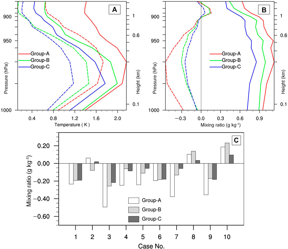
FIGURE 4. Average vertical profiles of the RMSE (solid lines) and biases (dash lines) between the 12-h forecast and the radiosonde observations in Figure 1 for (A) temperature, (B) mixing ratio, and (C) the bias of the mixing ratio profiles averaged from the surface to 850 hPa for the 10 cases.

These aforementioned results are in line with our idea for the proposal of the revised method. Although it performs better than the W14 method, for some cases, the extent of its improvement is still not very satisfactory. For instance, the BS of cases 5, 8, and 9 are 1.487, 1.655, and 1.555, respectively (Table 2). Next, we take case 3 as an example to discuss the working mechanism of the revised method. Case 3 is chosen because it has the largest dry bias after assimilating obs only and the effect of the revised method relative to the W14 method is not obvious (Figure 4C).

5 Case study

5.1 Sensitivity experiments

Sea fog of case 3 is a typical advection fog that began to occur over the junction of the Yellow Sea and East China Sea under the control of high pressure in the evening of 28 April, 2008 (Figure 5A). The Yellow Sea was dominated by weak southerly winds, and high pressure changed little until the next morning (figure not shown), transporting the warm moist air mass northward to promote sea fog developing northward (Figure 5B; nighttime fog was detected by the algorithm in the W14 method). Till 2000, LST 29 April, the high pressure strengthened and moved eastward slightly, and the sea fog almost occupied the entire Yellow Sea and bordered on the west bank of the Korean Peninsula. (Figures 5C,D). The detailed evolution of the sea fog is shown in Figure 6 (see the first row; daytime fog is directly denoted by visible images). Forced by the intensified pressure gradient, the southerly wind became stronger, and then dissipated the south part of the fog patch.

FIGURE 5

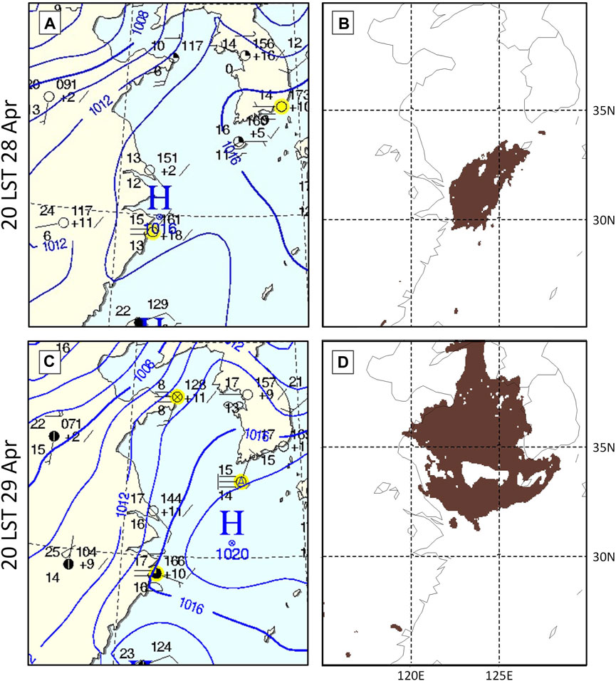
FIGURE 5. Surface synoptic chart (left; (A,C) and MTSAT-detected fog patch (right; (B,D) at 20 LST 28 April 2008 (upper; (A,B) and 20 LST 29 April 2008 later (bottom; (C,D).

FIGURE 6

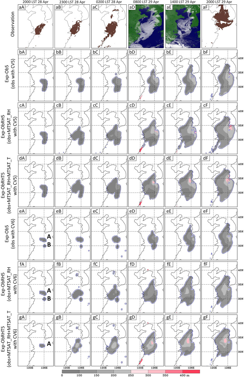
FIGURE 6. Comparison between the observed and simulated fog areas. Time for each column is placed on the top. The first row is the satellite-observed sea fog, among which MTSAT-visible cloud images are used for daytime fog and the MTSAT-derived fog area with thickness height denotes nighttime fog. The second to seventh rows show the simulated fog area with thickness for the experiments where names are given on the left marginal side. The fog patches marked with A in (eA), (fA), and (gA) are related to the hit fog area, while the patches marked with B in (eA) and (fA) are literally spurious. These patches are referred in detail in Section 5.2.1.

As mentioned in Section 3.2 about BE (CV5 and CV6), the multivariate cross-correlations among control variables in BE are important to sea fog modeling (Gao and Gao 2020). The aforementioned experiments employed CV5, which has no cross-correlation between moisture and other control variables, such as temperature. In the revised method, the added temperature constraint is mainly used for better conversion of RH to Qv. If CV5 is used, assimilations of moisture (QV) and temperature are completed independently. On the contrary, if CV6 is used, assimilation of temperature can directly affect humidity. Therefore, we further conducted three sensitivity experiments: Exp-Ob6, Exp-ObRH6, and Exp-ObRHT6. Note that the letters Ob and RH and the number six in these experimental names denote the assimilation of obs, assimilation of MTSAT-RH, and employment of CV6 in the experiments, respectively. Similarly, the experiments for case 3 in Group-A, Group-B, and Group-C are named as Exp-Ob5, Exp-ObRH5, and Exp-ObRHT5, respectively.

5.2 Results analysis

5.2.1 Simulated fog area

The simulated fog areas of the sensitivity experiments were evaluated. Table 3 shows the statistical scores of POD, FAR, BS, and ETS. For comparison, the results of Exp-Ob5, Exp-ObRH5, and Exp-ObRHT5 are also shown in Table 3.

TABLE 3

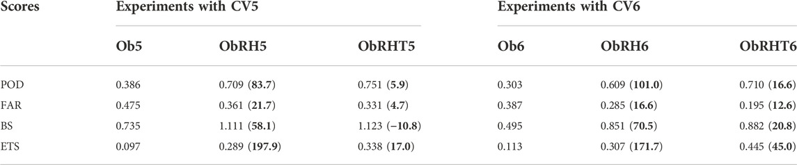
TABLE 3. Statistical scores for each experiment in the case study. Numbers in parentheses for Exp-ObRH5/6 show the improvements (%) relative to Exp-Ob5/6, while those for Exp-ObRHT5/6 show the improvements relative to Exp-ObRH5/6.

As shown in Table 3, POD for Exp-Ob5 is only 0.386 and its BS is 0.735, indicating that the simulated fog area is about 25% smaller than the observed one. Because of the assimilation of MTSAT-RH, all the four scores improved in Exp-ObRH5, for example, POD increased up to 0.709 and BS changed to 1.111, meaning that the simulated fog area was about 11% larger than the observed one. ETS of Exp-ObRHT5 improved by 17% relative to Exp-ObRH5, resulting from the temperature constraint. However, BS of Exp-ObRHT5 got worse relative to Exp-ObRH5. For those experiments with CV6, all scores of Exp-ObRH6 were significantly better than those of Exp-Ob6, and so is Exp-ObRHT6 relative to Exp-ObRH6. ETS of Exp-Ob5 is dramatically raised from 0.097 to 0.445 in Exp-ObRHT6, owing to benefits from the assimilation of MTSAT-RH using CV6 with the temperature constraint. The BS deterioration of Exp-ObRHT5 relative to Exp-ObRH5 does not occur in the similar experiments with CV6. Results of Table 3 indicate that the revised method with CV6 performs much better than with CV5, and the relative improvement rate reaches 45%.

Figure 6 presents the comparison between the observed fog area and simulated fog area. The observed fact (the first row in Figure 6) shows that the sea fog formed over the southern Yellow Sea with a small patch (Figure 6A), slowly extending northward and then almost covering the entire Yellow Sea (Figures 6aB–aE). At the same time, the southern part of the sea fog retreated slightly northward (Figure 6aF). This evolution process is basically captured by all experiments (cf. the first row and the other rows in Figure 6). The simulation effect of Exp-ObRHT6 is the best because both the northward expansion of the fog area and the contraction of its southern part are the closest to the observed facts (cf. the panels of the rightmost column in Figure 6).

Compared with the observed fog area at 2000 LST 28 April (Figure 6A), there was a large proportion of spurious fog in the simulated fog area of the experiments with CV5. The spurious fog did not disappear in the next 3 h (e.g., Figure 6dB). By comparison, the experiments with CV6 had obviously different simulated fog areas at 2000 LST 28 April (e.g., Figure 6eA). In Exp-Ob6 and Exp-ObRH6, the fog area included two patches, among which the patch marked with B was literally spurious (Figures 6eA, fA). However, this spurious patch did not exist in Exp-ObRHT6 (Figure 6gA). Within the next 3 h, the patch marked with A of Exp-ObRHT6 gradually grew, and its shape was very close to that of the observed fog area (cf. Figures 6gB and 6aB), and the subsequent sea fog was also closer to the observed fact than all the other experiments (e.g., the third column in Figure 6). It indicates that the revised method needs to cooperate with CV6 to have better effect.

5.2.2 Structure of the marine atmospheric boundary layer

Similar to the analysis in Section 4.2, the 00-h and 12-h forecast bias profiles of temperature and mixing ratio within the MABL were compared with the coastal radiosonde observations (see their sites in Figure 1). Similar to the profiles in Figure 4, the comparison results demonstrated that the RMSEs of both temperature and mixing ratio for Exp-ObRH5/6 were smaller than those of Exp-Ob5/6, respectively (Figure 7), and it is the same for Exp-ObRHT5/6 relative to Exp-ObRH5/6, respectively. For intuitively and quantitatively evaluating the temperature and humidity structure of MABL simulated by the six experiments, the profiles of biases and RMSEs are averaged from 1,000 hPa to 950 hPa, and the results are listed in Table 4.

FIGURE 7

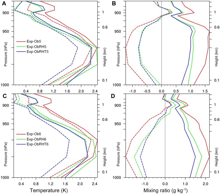
FIGURE 7. As in Figures 4A, B, the time of 2000 LST 28 April 2008 and (A) and (B) are for Exp-Ob5, Exp-ObRH5, and Exp-ObRHT5, and (C) and(D) are for Exp-Ob6, Exp-ObRH6, and Exp-ObRHT6.

TABLE 4

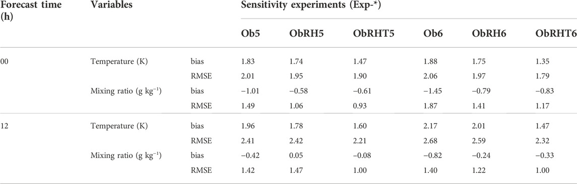
TABLE 4. Average biases and RMSEs of the temperature and mixing ratio from 1,000 hPa to 950 hPa at the 00-h and 12-h forecasts for verifying against the seven radiosonde observations around the Yellow Sea (see Figure 1).

As can be seen from Table 4, compared with Exp-Ob5/6 without assimilation of MTSAT-RH, the large dry biases at 00-h forecast (i.e., initial time) in Exp-ObH5/6 are reduced by nearly 50% (from −1.01 g kg⁻¹ to −0.58 g kg⁻¹ for Exp-ObH5, and from −1.45 g kg⁻¹to −0.79 g kg⁻¹for Exp-ObH6), resulting in the moisture status of the MABL at 12-h forecast getting improved (e.g., −0.58 g kg⁻¹ at 00-h forecast becomes 0.05 g kg⁻¹ at 12-h forecast for Exp-ObRH5). The dry bias of Exp-ObHT6 is basically equivalently to that of Exp-ObHT5 at both 00-h and 12-h forecasts. Whether CV5 or CV6 is used, the RMSE of the mixing ratio of the experiment with temperature constraint is the smallest. As for the profile of temperature, at the 00-h forecast, Exp-ObRHT6 has the smallest bias and RMSE in all experiments (1.35 and 1.79 K, respectively), and the bias at the 12-h forecast is also the smallest (1.47 K). It suggests that the temperature constraint can improve the temperature and humidity structure of MABL; particularly, the usage of CV6 can further help significantly improve the temperature structure of MABL.

In addition, in order to evaluate the forecasted humidity structure over sea, we compared the PW of model results (simulated PW) with that of satellite–bone microwave image observation (observed PW). The simulated PW was interpolated onto the horizontal grids of the observed PW to facilitate point-to-point statistics. Considering the system bias of the observed PW and its retrieval algorithm, the correlation between the simulated PW and the observed PW is as important as their mean difference (i.e., bias) because it shows the model’s ability to predict the pattern of water vapor. The correlation coefficient was calculated within the forecasted fog areas:

$\rho =\frac{\frac{1}{n}\sum \left[{pw}_f\left(i,j\right)-\overline{{pw}_f}\right]\left[{pw}_o\left(i,j\right)-\overline{{pw}_o}\right]}{\sqrt{\frac{1}{n}\sum {\left[{pw}_f\left(i,j\right)-\overline{{pw}_f}\right]}^2}\sqrt{\frac{1}{n}\sum {\left[{pw}_o\left(i,j\right)-\overline{{pw}_o}\right]}^2}},(10)$

where ${pw}_f$ and ${pw}_o$ are simulated and observed PW, respectively; and the sum was done at all the grid points within the simulated fog whose total number was $n$ (missing values for observation were excluded). Figure 8 presents the mean bias (color shades) and correlation coefficient (number in bottom-left corner of each panel) of PW for all experiments. At approximately 6-h, 9-h, 10-h, and 11-h forecasts, the corresponding observed PW was provided by AMSR-E, SSM/I, SSMIS, and WindSAT, respectively.

FIGURE 8

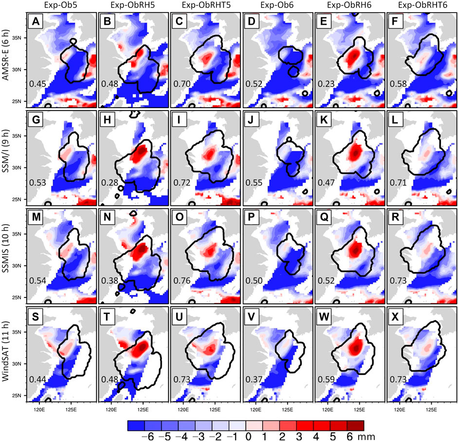
FIGURE 8. Bias (color shades) and correlation coefficient (number on the bottom-left corner of each panel) between the simulated and satellite-observed precipitable waters within the simulated fog area that is outlined by a thick black line. Experiment names are shown on the top, and forecast hours related with the satellite sensor are given on the left marginal side. Panels (A–F) show the comparison between Exp-Ob5, Exp-ObRH5, Exp-ObRHT5, Exp-Ob6, Exp-ObRH6, Exp-ObRHT6, and AMSR-E observation at the 6-h forecast (1400 LST 29 April), respectively. Similarly, panels (G–L) are for SSM/I observation at the 9-h forecast, panels (M–R) are for SSMIS observation at the 10-h forecast, and panels (S–X) are for WindSAT observation at the 11-h forecast.

Looking through the correlation coefficients given in Figure 8, it is found that only half of the coefficients improved in Exp-ObRH5/6 after assimilating MTSAT-RH together with obs, while all coefficients greatly increased in Exp-ObRHT5/6 with the temperature constraint (cf. the numbers in the third/sixth column and those in the first/fourth column, respectively). Through contrasting the biases (color shades), it can be seen that Exp-Ob5 and Exp-Ob6 have dry biases (see blue colors) in most of the observed fog areas (outlined by coarse lines), while small wet biases only partially existed (see red colors). At the 06-h forecast, the bias in the fog area was between −10.33 and 3.93 mm for Exp-Ob5 (Figure 8A) and between −12.33 and −0.68 mm for Exp-Ob6 (Figure 8D), and the mean value for Exp-Ob5/6 was −5.11/−7.13 mm. At the 09-h forecast, the mean bias for Exp-Ob5/6 was −3.43/−5.21 mm (Figures 8G, I). After assimilation of MTSAT-RH in Exp-ObRH5/6, these dry biases were overcorrected and significant large wet biases resided in most of the observed fog areas (e.g., see the red shadings in Figures 8N, Q, T, W). The temperature constraint with CV5 slightly alleviated the large wet biases (e.g., cf. Figures 8H, I), whereas the wet biases greatly decreased under the temperature constraint with CV6 (e.g., cf. Figures 8K, L). In Exp-ObRHT6, there are slight wet biases (∼1 mm) in most of the observed fog areas, and the correlation coefficients vary from 0.58 to 0.73, which indicates that the moisture status is successfully simulated during the fog evolution.

The aforementioned results show the importance of the temperature constraint with CV6 in the assimilation of MTSAT-RH in the revised method. The next subsection explains how the improvements in Exp-ObRHT6 are achieved.

5.3 Role of CV6 for the revised method

To investigate the reason why Exp-ObRHT6 has a better performance than Exp-ObRHT5, we looked at the insight into the analysis increments at the model bottom level of the 3DVAR update (see Figure 3B). Figure 9 shows the analytic increments of temperature and moisture at the final 3DVAR update for Exp-ObRH5/6 (Figures 9A, D), Exp-ObRHT5/6 (Figures 9B, E), and the differences between Exp-ObRHT5/6 and Exp-ObRH5/6 (Figures 9C, F). In Figure 9, the observed fog area is outlined by the thick black line, and the thick dash line is for the simulated fog area. The areas of hit fog, missed fog, and false fog are denoted by H, M, and F, respectively. The missed fog and hit fog areas of Exp-ObRH5 and Exp-ObRH6 are almost the same; however, their false fog areas differ greatly (see H, M, and F in Figures 9A, D). The false fog area still appears in Exp-ObRHT5 after assimilating MTSAT-RH with the temperature constraint (cf. Figures 9A, B), but almost disappears in Exp-ObRHT6 (cf. Figures 9D, E).

FIGURE 9

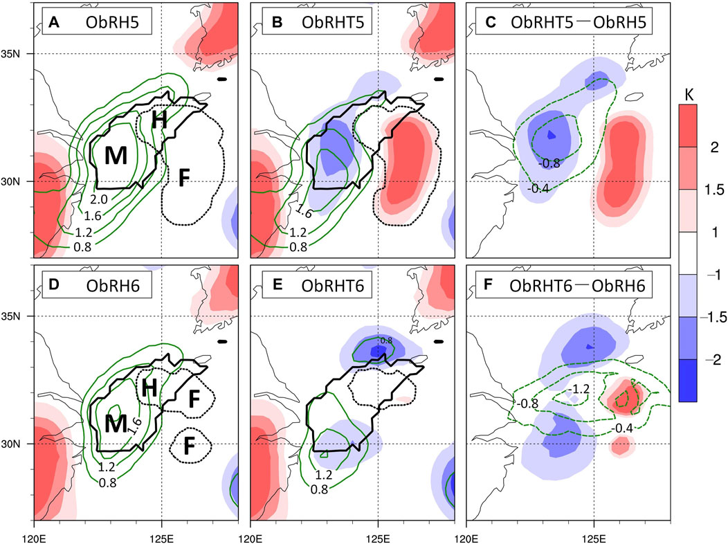
FIGURE 9. Analysis increments at the initial time for Exp-ObRH5 (A), Exp-ObRHT5 (B), Exp-ObRH5 (D), and Exp-ObRHT5 (E) at the model bottom level. (C,D) are Exp-ObRHT5 minus Exp-ObRH5 and Exp-ObRHT6 minus Exp-ObRH6 (F), respectively. Shadings, green contours denote the temperature (K), mixing ratio (g kg⁻¹), respectively. Black solid and dashed lines outline the observed and forecasted fog areas, respectively. M, H, and F denote the missed fog, hitting fog and false fog, respectively.

Overviewing the increment distribution in Figure 9, it is found that 1) Exp-ObRH5/6 only has analytic increments of the mixing ratio related to the observed fog area (Figures 9A, D) because the temperature in humidity sounding (Figure 2A) is extracted from the analysis, leading to no observable increment of temperature in the 3DVAR update; 2) Exp-ObRHT5/6 has analysis increments of both mixing ratio and temperature (Figures 9B, E, C, F), owing to the temperature constraint in the revised method; 3) compared with Exp-ObRH5/6, Exp-ObRHT5/6 has a more accurate coverage over the observed fog area and its maximum is about 0.4 g kg⁻¹ smaller (cf. the green contours of Figures 9A, D, B, E, respectively), which is contributed from the cross-correlation between moisture and temperature in CV6.

Because of the positive increments of mixing ratio over the missed fog area (M in Figures 9A, D), 3 h later, sea fog occurred over the missed fog area (e.g., cf. Figures 6cA and cB, fA and fB, etc.). It means that both the W14 method and revised method do work on compensating the missed fog area. However, the revised method only using CV6 is effective for eliminating the false fog area. For instance, the southern patch of the missed fog area denoted by F in Figure 9D does not appear in Figure 9E. Benefitting from the correction of the temperature profile in the nearest clear air area replacing that in the false fog area (see Figure 3A), there are positive temperature increments over the false fog area (e.g., see the red shadings in Figures 9C, F), which is beneficial to dissipate the false fog area. However, positive temperature increment is not enough to eliminate the false fog area. It seems that the reason that the false fog area only dissipates in Exp-ObRHT6 is that, relative to Exp-ObRH6, there are extra negative increments of the mixing ratio over its false fog area, which does not exist in Exp-ObRHT5 relative to Exp-ObRH5 (see the green contours in Figures 9C, F).

Figure 10 presents the distributions of 2-m temperature, 10-m wind, and 2-m RH with a value of 95% for roughly denoting the simulated fog area, 2-m mixing ratio, and geopotential height at 1,000 hPa level. According to the observed fog area (Figure 3B) and the simulated fog area of Exp-Ob6 (Figure 6eA), two areas designated by blue and red boxes are used to determine the missed fog area and false fog area, respectively. The missed fog in Exp-Ob6 appears in both Exp-ObRH6 and Exp-ObRHT6, resulting from the existence of the wet tongue of the mixing ratio (Figures 10B, E). Although the wet tongue of Exp-ObRHT6 is weaker than that of Exp-ObRH6 (cf., Figures 10E, F), its simulated fog expands more northward and is closer to the observation, which results from a stronger sea surface wind (1–2 m s⁻¹ larger) by the enhanced high-pressure system. This is obviously seen from the comparison of the geopotential heights between Figures 10B, C, E, F, respectively. This shows that in addition to the aforementioned advantages, the temperature constraint with CV6 can also provide a more accurate low-level pressure system. As a result of the enhanced high-pressure system in Exp-ObRHT6, a drier area of the mixing ratio exists over the false fog area than Exp-ObRH6, which leads to the elimination of its false fog.

FIGURE 10

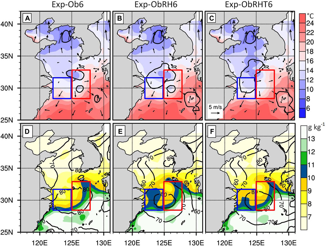
FIGURE 10. Distributions of 2-m temperature and 10-m wind [shades and vectors in (A–C)], and 2-m mixing ratio and geopotential height at 1,000 hPa level [shades and contours in (D–F)]. In (A–C), the contour of 2-m RH with a value of 95% roughly outlines the simulated fog area. See the text for details of the blue and red boxes in each panel.

To check the impact of the temperature constraint with CV6 on the vertical structure of MABL, the profiles of temperature and mixing ratio of 00-h forecast (i.e., the initial condition) within the false and missed fog areas were collected and averaged. For unifying the number and locations of the profile samples, the false and missed fog areas were determined according to the comparison of the observed fog area and the simulated fog area by Exp-ObRH6 (see the areas denoted by M and F in Figure 9D). Figure 11 gives the averaged profiles of Exp-ObRH6 and Exp-ObRHT6 within MABL, showing that the difference of temperature profiles (Figures 11A, B) between Exp-ObRH6 and Exp-ObRHT6 is apparently larger than that of the mixing ratio profiles (Figures 11C, D) for both the false area and the missed fog area. In the false fog area, the temperature profile of Exp-ObRHT6 is about 1.5 K warmer than that of Exp-ObRH6 within 100 m (Figure 11A), and the overall mixing ratio profile of Exp-ObRHT6 is about 0.5 g kg^-1 drier than that of Exp-ObRH6, contributing to the elimination of the false fog area. In spite of the fact that the overall mixing ratio profile of Exp-ObRHT6 is 0.5–1.0 g kg^-1 drier than that of Exp-ObRH6, the mixing ratio is still 8.5–9.5 g kg^-1. In addition, the temperature profile of Exp-ObRHT6 is nearly 2.5 K colder than that of Exp-ObRH6, and the stability becomes nearly neutral from the strong inversion within 200 m, which is beneficial to the subsequent fog formation over the missed fog area.

FIGURE 11

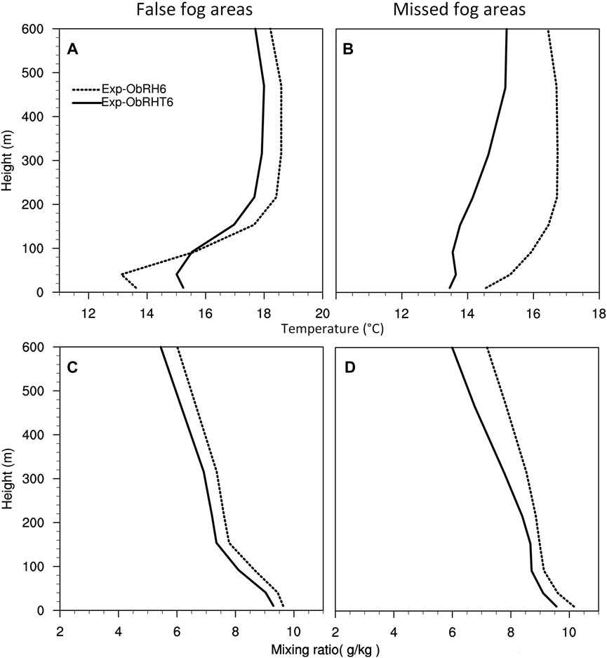
FIGURE 11. Average profiles of the 00-h forecasted air temperature within the areas of false fog (A) and missed fog (B), as well as the average profiles of the mixing ratio within the areas of false fog (C) and missed fog (D). Solid and dash lines denote Exp-ObRHT6 and Exp-ObRH6, respectively. Note that the missed fog and false fog areas are determined by the comparison of the observed fog and the simulated fog from Exp-ObRH6 (see Figure 9D).

6 Summary

Sea fog forecast is sensitive to initial conditions because the formation and evolution of sea fog over the Yellow Sea are strongly affected by the thermal structure of MABL. To solve the deficiency of MABL moisture for the Yellow Sea forecast, Wang et al. (2014) developed the W14 method to assimilate satellite-derived humidity. This method can significantly improve the sea fog forecast. However, it causes much moisture into initial conditions and ignores dealing with spurious fog area, which produces wet bias and increases false alarms. For alleviating this problem, we proposed a revised method with the temperature constraint based on the W14 method. In the new method, the temperature given for a humidity sounding is not directly extracted from the 3DVAR analysis, but from the nearest fog area. In addition, the revised method also intends to eliminate spurious fog by adding the temperature provided from the nearest clear air area.

A series of numerical forecast experiments were conducted for 10 sea fog cases that occurred over the Yellow Sea to evaluate the revised method’s effect, and one of the cases was selected for a case study to explore the impact of temperature constraint in the revised method. In the case study, we especially compared the assimilation effect of using CV5 and CV6, while in the aforementioned experiments for 10 cases, CV5 was used to be consistent with the W14 method. The main conclusions are as follows:

1) The revised method outperforms the W14 method. The moisture and temperature structure in the MABL is more realistic, and the large wet bias in the W14 method can be greatly alleviated. The comprehensive score ETS is increased by about 15% on average, which is due to the significant improvement brought by the reduction of the false fog area.

2) The benefits of the revised method are mainly reflected in two aspects: one is to make up for the missed fog area and the other is to eliminate the false fog area. The temperature constraint cools MABL in the missed fog area and warms that in the false one, which helps sea fog develop as accurately as possible.

3) The effect of the revised method depends largely on the BE type used in the 3DVAR, and its performance using CV6 is much better than that using CV5. In the experiment with CV5, the false fog area is hardly eliminated, while it is eliminated well in the experiment with CV6 due to the contributions by the cross-correlations between temperature and humidity in CV6. It indicates that the revised method jointly with CV6 is probably a better solution for sea fog forecast.

Although this study has achieved encouraging results, it should be emphasized that the retrieval of sea fog needs to be improved, and the current treatment process of temperature constraints is somewhat rough. More work needs to be done to improve the revised method. On the other hand, multivariate BE covariance is seldom used in the sea fog forecast. Performance of the revised method with CV6 is to be evaluated in more cases which occur not only over the Yellow Sea, but also over other Chinese seas. We hope that the revised method in this study can be applied into the operational forecast of sea fog in the future.

Data Availability Statement

The original contributions presented in the study are included in the article/Supplementary Material; further inquiries can be directed to the corresponding authors.

Author contributions

XG: Formal analysis; methodology and software; and writing—original draft. SG and YW: Conceptualization; supervision; and writing—review and editing. ZL: Data curation and resources. All authors discussed the results and commented on the manuscript.

Funding

This research was financially supported by the National Natural Science Foundation of China (42075069).

Acknowledgments

We would like to thank the reviewers for their helpful comments and suggestions that improved the manuscript.

Conflict of interest

The authors declare that the research was conducted in the absence of any commercial or financial relationships that could be construed as a potential conflict of interest.

Publisher’s note

All claims expressed in this article are solely those of the authors and do not necessarily represent those of their affiliated organizations, or those of the publisher, the editors, and the reviewers. Any product that may be evaluated in this article, or claim that may be made by its manufacturer, is not guaranteed or endorsed by the publisher.

Abbreviations

CV5, a kind of background error covariance, in which moisture is an independent control variable and not correlated to other control variables; CV6, as CV5, but moisture is correlated to other control variables; MTSAT-RH, artificial humidity soundings within the fog area detected from MTSAT (see Figure 2A); MTSAT-T, artificial temperature soundings within the areas of hit, missed, and false sea fog (see Figure 3); obs, routine observations, including measurements from upper-air radiosondes, surface stations, and a small amount of satellite-retrieved temperature and humidity profiles; Exp-Ob5, the numerical experiment for Case 3 (the sea fog occurred in April 2008), in which only obs is assimilated with CV5. Ob5 denotes obs and CV5; Exp-Ob6, as Exp-Ob5, but CV6 is used instead of CV5; Exp-ObRH5, as Exp-Ob5, but MTSAT-RH is assimilated together with obs by using the W14 method. RH denotes MTSAT-RH; Exp-ObRH6, as Exp-ObRH5, but CV6 is used instead of CV5; Exp-ObRHT5, as Exp-ObRH5, but MTSAT-T is added into the assimilation of obs and MTSAT-RH by the revised method; Exp-ObRHT6, as Exp-ObRHT5, but CV6 is used instead of CV5; Group-A, the group of numerical experiments for 10 cases, assimilating obs only; Group-B, as Group-A, assimilating obs and MTSAT-RH by the W14 method; Group-C, as Group-A, assimilating obs, MTSAT-RH, and MTSAT-T by the revised method.

References

Ballard, S. P., Golding, B. W., and Smith, R. N. B. (1991). Mesoscale model experimental forecasts of the haar of northeast Scotland. Mon. Wea. Rev. 119, 2107–2123. doi:10.1175/1520-0493(1991)119<2107:mmefot>2.0.co;2

CrossRef Full Text | Google Scholar

Bendix, J., Thies, B., Cermak, J., and Nauß, T. (2005). Ground fog detection from space based on MODIS daytime data—a feasibility study. Weather Forecast. 20, 989–1005. doi:10.1175/waf886.1

CrossRef Full Text | Google Scholar

Chen, F., and Dudhia, J. (2001). Coupling an advanced land surface–hydrology model with the penn state–NCAR MM5 modeling system. Part I: Model implementation and sensitivity. Mon. Wea. Rev. 129, 569–585. doi:10.1175/1520-0493(2001)129<0569:caalsh>2.0.co;2

CrossRef Full Text | Google Scholar

Ellrod, G. P. (1995). Advances in the detection and analysis of fog at night using GOES multispectral infrared imagery. Wea. Forecast. 10, 606–619. doi:10.1175/1520-0434(1995)010<0606:aitdaa>2.0.co;2

CrossRef Full Text | Google Scholar

Findlater, J., Roach, W. T., and McHugh, B. C. (1989). The haar of north-east Scotland. Q. J. R. Meteorol. Soc. 115, 581–608. doi:10.1002/qj.49711548709

CrossRef Full Text | Google Scholar

Fu, G., Xu, J., and Zhang, S. Q. (2011). Comparison of modeling atmospheric visibility with visible satellite imagery. J. Ocean. Univ. China 41, 001–010. (in Chinese). doi:10.16441/j.cnki.hdxb.2011.04.002

CrossRef Full Text | Google Scholar

Fu, G., Zhang, S. P., Gao, S. H., and Li, P. Y. (2012). Understanding of sea fog over the China seas. Beijing: China Meteorological Press, 220.

Google Scholar

Gao, X., and Gao, S. (2019). EnKF assimilation of cloud water path in nowcasting sea fog over the Yellow Sea (in Chinese). Oceanol. Limnol. Sin. 50 (2), 248–260.

Google Scholar

Gao, X., and Gao, S. (2020). Impact of multivariate background error covariance on the WRF-3DVAR assimilation for the Yellow Sea fog modeling. Adv. Meteorol. 2020, 1–19. doi:10.1155/2020/8816185

CrossRef Full Text | Google Scholar

Gao, S. H., Lin, H., Shen, B., and Fu, G. (2007). A heavy sea fog event over the Yellow Sea in March 2005: Analysis and numerical modeling. Adv. Atmos. Sci. 24, 65–81. doi:10.1007/s00376-007-0065-2

CrossRef Full Text | Google Scholar

Gao, S. H., Wu, W., Zhu, L. L., Fu, G., and Huang, B. (2009). Detection of nighttime sea fog/stratus over the Huanghai Sea using MTSAT-1R IR data. Acta Oceanol. Sin. 28, 23–35. doi:10.3969/j.issn.0253-505X.2009.02.003

CrossRef Full Text | Google Scholar

Gao, S. H., Qi, Y. L., Zhang, S. B., and Fu, G. (2010). Initial conditions improvement of sea fog numerical modeling over the Yellow Sea by using cycling 3DVAR. Part I: WRF numerical experiments (in Chinese). J. Ocean. Univ. China 40, 001–009. doi:10.16441/j.cnki.hdxb.2010.10.001

CrossRef Full Text | Google Scholar

Gao, X., Gao, S., and Yang, Y. (2018). A comparison between 3DVAR and EnKF for data assimilation effects on the Yellow Sea fog forecast. Atmosphere 9, 346. doi:10.3390/atmos9090346

CrossRef Full Text | Google Scholar

Gultepe, I., Tardif, R., Michaelides, S. C., Cermak, J., Bott, A., Bendix, J., et al. (2007). Fog research: A review of past achievements and future perspectives. Pure Appl. Geophys. 164, 1121–1159. doi:10.1007/s00024-007-0211-x

CrossRef Full Text | Google Scholar

Heidinger, A. K., and Stephens, G. L. (2000). Molecular line absorption in a scattering atmosphere. Part II: Application to remote sensing in the O₂ A band. J. Atmos. Sci. 57, 1615–1634. doi:10.1175/1520-0469(2000)057<1615:mlaias>2.0.co;2

CrossRef Full Text | Google Scholar

Hong, S. Y., Noh, Y., and Dudhia, J. (2006). A new vertical diffusion package with an explicit treatment of entrainment processes. Mon. Weather Rev. 134, 2318–2341. doi:10.1175/mwr3199.1

CrossRef Full Text | Google Scholar

Hong, S. Y. (2010). A new stable boundary-layer mixing scheme and its impact on the simulated East Asian summer monsoon. Q. J. R. Meteorol. Soc. 136, 1481–1496. doi:10.1002/qj.665

CrossRef Full Text | Google Scholar

Hu, X. M., Klein, P. M., and Xue, M. (2013). Evaluation of the updated YSU planetary boundary layer scheme within WRF for wind resource and air quality assessments. J. Geophys. Res. Atmos. 118 (18), 10490–10505. doi:10.1002/jgrd.50823

CrossRef Full Text | Google Scholar

Huang, H., Liu, H., Huang, J., Mao, W., and Bi, X. (2015). Atmospheric boundary layer structure and turbulence during sea fog on the southern China coast. Mon. Weather Rev. 143, 1907–1923. doi:10.1175/mwr-d-14-00207.1

CrossRef Full Text | Google Scholar

Iacono, M. J., Delamere, J. S., Mlawer, E. J., Shephard, M. W., Clough, S. A., and Collins, W. D. (2008). Radiative forcing by long-lived greenhouse gases: Calculations with the AER radiative transfer models. J. Geophys. Res. 113, D13103. doi:10.1029/2008jd009944

CrossRef Full Text | Google Scholar

Kain, J. S., and Fritsch, J. M. (1990). A one-dimensional entraining/detraining plume model and its application in convective parameterization. J. Atmos. Sci. 47, 2784–2802. doi:10.1175/1520-0469(1990)047<2784:aodepm>2.0.co;2

CrossRef Full Text | Google Scholar

Kim, C. K., and Yum, S. S. (2010). Local meteorological and synoptic characteristics of fogs formed over Incheon international airport in the west coast of Korea. Adv. Atmos. Sci. 27 (4), 761–776. doi:10.1007/s00376-009-9090-7

CrossRef Full Text | Google Scholar

Kim, C. K., and Yum, S. S. (2012). A numerical study of sea-fog formation over cold sea surface using a one-dimensional turbulence model coupled with the weather research and forecasting model. Bound. Layer. Meteorol. 143 (3), 481–505. doi:10.1007/s10546-012-9706-9

CrossRef Full Text | Google Scholar

Kim, S., Moon, J. H., and Kim, T. (2021). A coupled numerical modeling study of a sea fog case after the passage of Typhoon Muifa over the Yellow Sea in 2011. Geophys. Res. Atmos. 126, e2020JD033875. doi:10.1029/2020jd033875

CrossRef Full Text | Google Scholar

Koračin, D., and Dorman, C. E. (2017). Marine fog: challenges and advancements in observations, modeling, and Forecasting. New York: Springer International Publishing, 537.

Google Scholar

Koračin, D., Lewis, J., Thompson, W. T., Dorman, C. E., and Businger, J. A. (2001). Transition of stratus into fog along the California coast: Observations and modeling. J. Atmos. Sci. 58, 1714–1731. doi:10.1175/1520-0469(2001)058<1714:tosifa>2.0.co;2

CrossRef Full Text | Google Scholar

Koračin, D., Businger, J. A., Dorman, C. E., and Lewis, J. M. (2005a). Formation, evolution, and dissipation of coastal sea fog. Bound. Layer. Meteorol. 117, 447–478. doi:10.1007/s10546-005-2772-5

CrossRef Full Text | Google Scholar

Koračin, D., Leipper, D. F., and Lewis, J. M. (2005b). Modeling sea fog on the U.S. California coast during a hot spell event. Geofizika 22, 59–82.

Google Scholar

Koračin, D., Dorman, C. E., Lewis, J. M., Hudson, J. G., Wilcox, E. M., and Torregrosa, A. (2014). Marine fog: A review. Atmos. Res. 143, 142–175. doi:10.1016/j.atmosres.2013.12.012

CrossRef Full Text | Google Scholar

Lewis, J. M., Koračin, D., Rabin, R., and Businger, J. (2003). sea fog off the California coast: Viewed in the context of transient weather systems. J. Geophys. Res. 108, 4457. doi:10.1029/2002jd002833

CrossRef Full Text | Google Scholar

Li, R., Gao, S. H., and Wang, Y. M. (2012). Numerical study on direct assimilation of satellite radiances for sea fog over the Yellow Sea (in Chinese). J. Ocean. Univ. China 42, 10–20. doi:10.16441/j.cnki.hdxb.2012.03.002

CrossRef Full Text | Google Scholar

Lin, Y. L., Farley, R. D., and Oriville, H. D. (1983). Bulk parameterization of the snow field in a cloud model. J. Clim. Appl. Meteor. 22, 1065–1092. doi:10.1175/1520-0450(1983)022<1065:bpotsf>2.0.co;2

CrossRef Full Text | Google Scholar

Liu, X., and Hu, X. Q. (2008). Sea fog automatic detection over the East China Sea using MTSAT data (in Chinese). J. Oceanogr. Taiwan 27, 112–117.

Google Scholar

Liu, Y. D., Ren, J. P., and Zhou, X. (2011). The impact of assimilating sea surface wind aboard QuickSCAT on sea fog simulation (in Chinese). J. Appl. Meteor. Sci. 22 (04), 472–481.

Google Scholar

Lorenz, E. N. (1965). A study of the predictability of a 28-variable atmospheric model. Tellus 17, 321–333. doi:10.1111/j.2153-3490.1965.tb01424.x

CrossRef Full Text | Google Scholar

Lu, X., Gao, S. H., Rao, L. J., and Wang, Y. M. (2014). Sensitivity study of WRF parameterization schemes for the spring sea fog in the Yellow Sea (in Chinease). J. Appl. Meteor. Sci. 25, 312–320.

Google Scholar

Nicholls, S. (1984). The dynamics of stratocumulus: Aircraft observations and comparisons with a mixed layer model. Quart. J. Roy. Meteor. Soc. 110, 783–820. doi:10.1002/qj.49711046603

CrossRef Full Text | Google Scholar

Parrish, D. F., and Derber, J. C. (1992). The National Meteorological Center’s spectral statistical-interpolation analysis system. Mon. Wea. Rev. 120, 1747–1763. doi:10.1175/1520-0493(1992)120<1747:tnmcss>2.0.co;2

CrossRef Full Text | Google Scholar

Skamarock, W. C., Klemp, J. B., Dudhia, J., Gill, D. O., Barker, D., Duda, M. G., et al. (2008). A description of the Advanced Research WRF version 3. Note NCAR/TN–4751STR. NCAR Tech. 113.

Google Scholar

Sorli, B., Pascal-Delannoy, F., Giani, A., Foucaran, A., and Boyer, A. (2002). Fast humidity sensor for high range 80%– 95% RH. Sens. Actuators 100, 24–31. doi:10.1016/S0924-4247(02)00063-8

CrossRef Full Text | Google Scholar

Wang, Y., and Gao, S. (2016). Assimilation of Doppler Radar radial velocity in Yellow Sea fog numerical modeling (in Chinese). J. Ocean. Univ. China 46, 1–12. doi:10.16441/j.cnki.hdxb.20150361

CrossRef Full Text | Google Scholar

Wang, Y., Gao, S., Fu, G., Sun, J., and Zhang, S. (2014). Assimilating MTSAT-derived humidity in nowcasting sea fog over the Yellow Sea. Weather Forecast. 29, 205–225. doi:10.1175/waf-d-12-00123.1

CrossRef Full Text | Google Scholar

Wang, B. H. (1985). Sea fog. Beijing: China Ocean Press, 330.

Google Scholar

Wu, X. J., Zhu, J., Wang, X., and Yang, B. (2017). Sea fog simulation with assimilation of FY-3A microwave data (in Chinese). Chin. J. Atmos. Sci. 41 (3), 421–436. doi:10.3878/j.issn.1006-9895.1610.16105

CrossRef Full Text | Google Scholar

Yang, Y., and Gao, S. H. (2015). Analysis on the synoptic characteristics and inversion layer formation of the Yellow Sea fogs (in Chinese). J. Ocean. Univ. China 45 (06), 19–30. doi:10.16441/j.cnki.hdxb.20140059

CrossRef Full Text | Google Scholar

Yang, Y., and Gao, S. H. (2020). The Impact of turbulent diffusion driven by fog-top cooling on sea fog development. J. Geophys. Res. Atmos. 125, e2019JD031562. doi:10.1029/2019jd031562

CrossRef Full Text | Google Scholar

Yang, Y., Hu, X., Gao, S., and Wang, Y. (2018). Sensitivity of WRF simulations with the YSU PBL scheme to the lowest model level height for a sea fog event over the Yellow Sea. Atmos. Res. 215, 253–267. doi:10.1016/j.atmosres.2018.09.004

CrossRef Full Text | Google Scholar

Yang, Y., Wang, Y., Gao, S., and Yuan, X. (2021). A new observation operator for the assimilation of satellite-derived relative humidity: Methodology and experiments with three sea fog cases over the Yellow Sea. J. Meteorol. Res. 35 (6), 1104–1124. doi:10.1007/s13351-021-1084-0

CrossRef Full Text | Google Scholar

Zhang, S. P., Xie, S. P., Liu, Q. Y., Yang, Y. Q., Wang, X. G., and Ren, Z. P. (2009). Seasonal variations of Yellow Sea fog: Observations and mechanisms. J. Clim. 22 (24), 6758–6772. doi:10.1175/2009jcli2806.1

CrossRef Full Text | Google Scholar

Zhou, B., and Du, J. (2010). Fog prediction from a multimodel mesoscale ensemble prediction system. Weather Forecast. 25, 303–322. doi:10.1175/2009waf2222289.1

CrossRef Full Text | Google Scholar

Zhou, F. X., Wang, X., and Bao, X. W. (2004). Climatic characteristics of sea fog formation of the Huanghai Sea in spring (in Chinese). Acta Oceanol. Sin. 26, 28–37.

Google Scholar