A new scheme of wavefield decomposed elastic least-squares reverse time migration

Elastic least-squares reverse time migration (ELSRTM) describes the reflectivity of the underground media more accurately than acoustic LSRTM in theory while suffering from the P- and S-waves crosstalk artifacts. We propose a new wavefield decomposed ELSRTM scheme to alleviate these crosstalk artifacts, which is different from conventional methods. In our new scheme, we implement the wavenumber domain elastic wavefield vector decomposition equivalently in the time-space domain to decompose source wavefield without Fourier transform, but with high precision. Then we decompose adjoint wavefield by constructing the shear component in a decoupled adjoint wave equation. Finally, based on elastic impedance parameterization, we derive the gradients with respect to elastic reflectivity in the wavefield-decomposed ELSRTM. Numerical examples show that our method is feasible even when applied to models with complex and uncorrelated P- and S-wave velocity structures.

1 Introduction

The work of several scholars marked the advent of reverse time migration (RTM) in the 1980s (Hemon, 1978; Baysal et al., 1983; McMechan, 1983; Whitmore, 1983). Compared with other migration methods, the reverse time migration based on the two-path wave equation has stronger amplitude preservation and higher image quality for the complex geological structure with steep dip angle and sharp velocity changes.

However, conventional RTM assumes that seismic data is obtained by regular surface sampling with a recording aperture as large as possible, which cannot be achieved in practice. Without these perfect assumptions, the conventional RTM algorithm is likely to fail even fed with accurate velocity and density models (Zhang et al., 2015).

The least square migration (LSM) (LeBras and Clayton, 1988) is a revolutionary innovation which solves imaging problems by an inversion method: match the observed data with the numerical simulation data under the Born approximation, and update the imaging results through multiple inversion iterations (Schuster, 1993; Nemeth et al., 1999). LSM is believed to be able to image subsurface structure and reflections with higher resolution and better amplitude preservation, which is beneficial to more reliable and high-precision elastic parameter inversion and reservoir characterization. The LSM idea can be combined with a variety of imaging techniques. Scholars have introduced the idea of LSM into RTM, which is called least-squares reverse time migration (LSRTM) (Dong et al., 2012; Yao and Jakubowicz, 2012; Dai and Schuster, 2013; Zhang et al., 2013, 2015; Feng and Schuster, 2017; Liu and Peter, 2018; Yang et al., 2019).

Most studies about LSRTM have been focused on acoustic medium assumptions, the elastic characteristics of the wavefield are treated as noise rather than an additional source of information of the subsurface parameters (Sears et al., 2010). However, elastic assumptions describe the underground media more accurately than acoustic. In addition, with PP and PS reflectivity, the identification of fluid contacts, lithologies, fractures and hydrocarbon reservoirs will be clear. Therefore, it is necessary to study LSRTM based on elastic theory for land seismic data. Considering that ELSRTM suffers from crosstalk between P- and S-waves, wavefield decomposition methods are usually used to suppress crosstalk artifacts.

One of the wavefield decomposition methods is based on the Helmholtz theorem (Dellinger and Etgen, 1990; Sun and McMechan, 2001), in a homogeneous and isotropic medium, the elastic wavefield can be separated into a curl-free P wavefield and a divergence-free S wavefield. However, extra complex and computationally expensive polarity corrections are needed since the divergence and curl operators lead to phase shift and amplitude distortion (Yan and Sava, 2008; Du et al., 2012; Duan and Sava, 2015).

The second strategy for wavefield decomposition is the decoupled wave equations (Ma and Zhu, 2003; Li et al., 2007; Zhang et al., 2007; Xiao and Leaney, 2010), which decompose wavefields by solving the P- and S-wave separated wave equations. In recent years, the decoupled wave equations prevail in elastic RTM (Wang and McMechan, 2015; Du et al., 2017; Zhou et al., 2018) and ELSRTM (Gu et al., 2018; Qu et al., 2018; Zhong et al., 2021; Shi et al., 2021; Zhang and Gao ,2022; Liu et al., 2022) because it is easy to implement and does not cause phase shift and amplitude distortion of decomposed wavefields (Duan and Sava, 2015; Du et al., 2017; Gong et al., 2018). However, if migration models are not smooth enough, the decoupled wave equation methods may suffer.

The third wavefield decomposition method, which with clear physical significance and higher accuracy, is the wavefields decomposition in the wavenumber domain (Zhang and McMechan, 2010; Du et al., 2014; Zhang et al., 2020), the output decomposed P- and S-wavefields have the same amplitude, phase, and physical units as the input wavefields even in the case of inaccurate migration velocity. However, methods in the wavenumber domain suffer from expensive computation.

Shi et al. (2021), Zhong et al. (2021), Zhang & Gao (2022) and Liu et al. (2022) constructed the decoupled wave equation and applied it to both source and adjoint wavefields decomposition. It is different in this paper: we propose a compound strategy to suppress P- and S-wave cross-talk artifacts in an efficient way. Inspired by the work of Zhang and McMechan (2010) in the wavenumber domain, but avoiding taking the Fourier transform, we reconstruct the wavenumber domain decomposition operator, and transform it into time-space domain to decompose source wavefields. Then we decompose the adjoint wavefields by constructing the shear component in a decoupled adjoint wave equation. Finally, we obtain the gradients with respect to elastic reflectivity in the wavefield-decomposed ELSRTM. In addition, the gradients were updated using the conjugate gradient method.

This paper is organized as follows. First, we review the basic theory of ELSRTM including the Born approximation for the velocity-stress elastic wave equations, the virtual sources of the elastic demigration, the adjoint equations and gradients of ELSRTM. Next, we introduce an elastic wavefield vector decomposition method in the time-space domain and a decoupled adjoint wave equation. Then we obtain the gradients with respect to elastic reflectivity in the decoupled P- and S-wave frame. Finally, we use two numerical examples to demonstrate the feasibility of the proposed wavefield decomposed ELSRTM scheme.

2 Methodology

2.1 Basic theory of ELSRTM

In the 2D case, the elastic isotropic wave equation can be expressed by the first-order particle velocity and stress equation (Virieux, 1986) as

$\begin{array}{l}\rho \frac{\partial v_x}{\partial t}=\frac{\partial {\sigma }_{xx}}{\partial x}+\frac{\partial {\tau }_{zx}}{\partial z},\\ \rho \frac{\partial v_z}{\partial t}=\frac{\partial {\tau }_{xz}}{\partial x}+\frac{\partial {\sigma }_{zz}}{\partial z},\\ \frac{\partial {\sigma }_{xx}}{\partial t}=\left(\lambda +2\mu \right)\frac{\partial v_x}{\partial x}+\lambda \frac{\partial v_z}{\partial z},\\ \frac{\partial {\sigma }_{zz}}{\partial t}=\lambda \frac{\partial v_x}{\partial x}+\left(\lambda +2\mu \right)\frac{\partial v_z}{\partial z},\\ \frac{\partial {\tau }_{xz}}{\partial t}=\mu \left(\frac{\partial v_x}{\partial z}+\frac{\partial v_z}{\partial x}\right).\end{array}(1)$

Where $\rho$ stands for the density, $\lambda$ and $\mu$ are the Lame constants of models, $v_x$ and $v_z$ represent particle velocities in the horizontal and vertical respectively, ${\sigma }_{xx}$ and ${\sigma }_{zz}$ are the normal stresses, ${\tau }_{xz}$ (or ${\tau }_{zx}$) is the shear stress.

According to the perturbation theory, a perturbation $\mathbf{\delta }\mathbf{m}={\left[\delta \rho ,\delta \lambda ,\delta \mu \right]}^T$ of the background model parameters $\mathbf{m}={\left[\rho ,\lambda ,\mu \right]}^T$ will lead to wavefields perturbation $\mathbf{\delta }\mathbf{u}={\left[\delta v_x,\delta v_z,\delta {\sigma }_{xx},\delta {\sigma }_{zz},\delta {\tau }_{xz}\right]}^T$ with respect to the background wavefields $\mathbf{u}={\left[v_x,v_z,{\sigma }_{xx},{\sigma }_{zz},{\tau }_{xz}\right]}^T$. The perturbed source wavefields which can be expressed as:

$\begin{array}{l}\rho \frac{\partial \delta v_x}{\partial t}-\frac{\partial \delta {\sigma }_{xx}}{\partial x}-\frac{\partial \delta {\tau }_{zx}}{\partial z}=f_x,\\ \rho \frac{\partial \delta v_z}{\partial t}-\frac{\partial \delta {\tau }_{xz}}{\partial x}-\frac{\partial \delta {\sigma }_{zz}}{\partial z}=f_z,\\ \frac{\partial \delta {\sigma }_{xx}}{\partial t}-\left(\lambda +2\mu \right)\frac{\partial \delta v_x}{\partial x}-\lambda \frac{\partial \delta v_z}{\partial z}=f_{xx},\\ \frac{\partial \delta {\sigma }_{zz}}{\partial t}-\lambda \frac{\partial \delta v_x}{\partial x}-\left(\lambda +2\mu \right)\frac{\partial \delta v_z}{\partial z}=f_{zz},\\ \frac{\partial \delta {\tau }_{xz}}{\partial t}-\mu \left(\frac{\partial \delta v_x}{\partial z}+\frac{\partial \delta v_z}{\partial x}\right)=f_{xz}.\end{array}(2)$

Where the virtual sources are as follows:

$\begin{array}{l}{f}_x=-\delta \rho \frac{\partial v_x}{\partial t},\\ f_z=-\delta \rho \frac{\partial v_z}{\partial t},\\ f_{xx}=\delta \lambda \left(\frac{\partial v_x}{\partial x}+\frac{\partial v_z}{\partial z}\right)+2\delta \mu \frac{\partial v_x}{\partial x},\\ f_{zz}=\delta \lambda \left(\frac{\partial v_x}{\partial x}+\frac{\partial v_z}{\partial z}\right)+2\delta \mu \frac{\partial v_z}{\partial z},\\ f_{xz}=\delta \mu \left(\frac{\partial v_x}{\partial z}+\frac{\partial v_z}{\partial x}\right).\end{array}(3)$

Equation 2 are the Born approximation for the velocity-stress elastic wave equation in the 2D case.

Using the adjoint-state method (Liu and Tromp, 2006; Plessix, 2006), the adjoint wave equations can be derived as:

$\begin{array}{l}\rho \frac{\partial {\varphi }_x}{\partial t}-\lambda \frac{\partial {\phi }_{zz}}{\partial x}-\left(\lambda +2\mu \right)\frac{\partial {\phi }_{xx}}{\partial x}-\mu \frac{\partial {\phi }_{xz}}{\partial z}=\delta V_x-\delta V_x^{obs},\\ \rho \frac{\partial {\varphi }_z}{\partial t}-\lambda \frac{\partial {\phi }_{xx}}{\partial z}-\left(\lambda +2\mu \right)\frac{\partial {\phi }_{zz}}{\partial z}-\mu \frac{\partial {\phi }_{xz}}{\partial x}=\delta V_z-\delta V_z^{obs},\\ \frac{\partial {\phi }_{xx}}{\partial t}-\frac{\partial {\varphi }_x}{\partial x}=0,\\ \frac{\partial {\phi }_{zz}}{\partial t}-\frac{\partial {\varphi }_z}{\partial z}=0,\\ \frac{\partial {\phi }_{xz}}{\partial t}-\left(\frac{\partial {\varphi }_x}{\partial z}+\frac{\partial {\varphi }_z}{\partial x}\right)=0.\end{array}(4)$

Here, $\varphi$ represents the adjoint wavefields of velocity, $\phi$ denotes the adjoint wavefields of stress, $\delta V_i$ and $\delta V_i^{obs}$, $i\in \left\{x,z\right\}$ represent the simulated and observed seismogram received in the horizontal (x) and vertical (z) directions respectively.

And gradients are derived as:

$\begin{array}{l}\frac{\partial J}{\partial \delta \rho }={\int }_0^T{\varphi }_x\frac{\partial v_x}{\partial t}+{\varphi }_z\frac{\partial v_z}{\partial t}dt,\\ \frac{\partial J}{\partial \delta \lambda }={\int }_0^T-\left({\phi }_{xx}+{\phi }_{\text{zz}}\right)\left(\frac{\partial v_x}{\partial x}+\frac{\partial v_z}{\partial z}\right)dt,\\ \frac{\partial J}{\partial \delta \mu }={\int }_0^T-\left(2{\phi }_{xx}\frac{\partial v_x}{\partial x}+2{\phi }_{zz}\frac{\partial v_z}{\partial z}+{\phi }_{xz}\left(\frac{\partial v_x}{\partial z}+\frac{\partial v_z}{\partial x}\right)\right)dt.\end{array}(5)$

2.2 The elastic wavefields decomposition

2.2.1 Decomposition of source wavefields

Zhang and McMechan (2010) proposed elastic wavefield decomposition in the wavenumber domain, which has been used to improve elastic full waveform inversion in Ren and Liu (2016). However, the two-dimensional forward and inverse Fourier transforms must be repeated in each time slice, resulting in expensive calculations. Different from Ren and Liu (2016), in our scheme, the work of Zhang and McMechan (2010) was introduced into the time-spatial domain, thereby avoiding the Fourier transforms, and was applied to ELSRTM efficiently.

The P- and S- wavefields in 2D case are decomposed in the wavenumber domain according to the following equations given by Zhang and McMechan (2010) as follows:

$\begin{array}{l}{\stackrel{\sim }{v}}_x^p\left(k_x,k_z\right)=K_x^2{\stackrel{\sim }{v}}_x\left(k_x,k_z\right)+K_x{K}_z{\stackrel{\sim }{v}}_z\left(k_x,k_z\right),\\ {\stackrel{\sim }{v}}_z^p\left(k_x,k_z\right)=K_z^2{\stackrel{\sim }{v}}_z\left(k_x,k_z\right)+K_x{K}_z{\stackrel{\sim }{v}}_x\left(k_x,k_z\right),\\ {\stackrel{\sim }{v}}_x^s\left(k_x,k_z\right)=K_z^2{\stackrel{\sim }{v}}_x\left(k_x,k_z\right)-K_x{K}_z{\stackrel{\sim }{v}}_z\left(k_x,k_z\right),\\ {\stackrel{\sim }{v}}_z^s\left(k_x,k_z\right)=K_x^2{\stackrel{\sim }{v}}_z\left(k_x,k_z\right)-K_x{K}_z{\stackrel{\sim }{v}}_x\left(k_x,k_z\right).\end{array}(6)$

where ${\stackrel{\sim }{v}}_x$ and ${\stackrel{\sim }{v}}_z$ represent particle velocities in the wavenumber domain, $K_x=k_x/k$ and $K_z=k_z/k$ are normalized wavenumbers, in which $\left(k_x,k_z\right)$ is the wavenumber vector that defines the direction of wave propagation in 2D case, and $k=\sqrt{k_x^2+k_z^2}=\omega /v_{pha}$, $v_{pha}$ is the phase velocity, $\omega$ denotes angular frequency. Zhang and McMechan (2010) further described Eq. 6 in a short form as:

$\begin{array}{l}{\stackrel{\sim }{\mathbf{V}}}^{\mathbf{P}}=\mathbf{K}\left(\mathbf{K}\cdot \stackrel{\sim }{\mathbf{V}}\right),\\ {\stackrel{\sim }{\mathbf{V}}}^{\mathbf{S}}=-\mathbf{K}\times \left(\mathbf{K}\times \stackrel{\sim }{\mathbf{V}}\right).\end{array}(7)$

where $\stackrel{\sim }{\mathbf{V}}={\stackrel{\sim }{\mathbf{V}}}^{\mathbf{P}}+{\stackrel{\sim }{\mathbf{V}}}^{\mathbf{S}}$, $\stackrel{\sim }{\mathbf{V}}=\left({\stackrel{\sim }{v}}_x,{\stackrel{\sim }{v}}_z\right)$, ${\stackrel{\sim }{\mathbf{V}}}^{\mathbf{P}}=\left({\stackrel{\sim }{v}}_x^p,{\stackrel{\sim }{v}}_z^p\right)$, ${\stackrel{\sim }{\mathbf{V}}}^{\mathbf{S}}=\left({\stackrel{\sim }{v}}_x^s,{\stackrel{\sim }{v}}_z^s\right)$, and we noticed that the operator $\mathbf{K}=K_x{\mathbf{a}}_{\mathbf{x}}+K_z{\mathbf{a}}_{\mathbf{z}}=\stackrel{\sim }{\nabla }/ik$, where $\stackrel{\sim }{\nabla }=i{k}_x{\mathbf{a}}_{\mathbf{x}}+i{k}_z{\mathbf{a}}_{\mathbf{z}}$ denotes the nabla operator in the wavenumber domain which corresponds to $\nabla =\partial /\partial x{\mathbf{a}}_{\mathbf{x}}+\partial /\partial z{\mathbf{a}}_{\mathbf{z}}$ in the spatial domain (${\mathbf{a}}_{\mathbf{x}}$ and ${\mathbf{a}}_{\mathbf{z}}$ are defined as unit basic vectors in the Cartesian coordinate system).

Naturally, set the intermediate results in parentheses as ${\stackrel{\sim }{V}}_{tmp}^P=\mathbf{K}\cdot \stackrel{\sim }{\mathbf{V}}$ and ${\stackrel{\sim }{\mathbf{V}}}_{\mathbf{t}\mathbf{m}\mathbf{p}}^{\mathbf{S}}=\mathbf{K}\times \stackrel{\sim }{\mathbf{V}}$, and note that $k={\omega /v}_{pha}$, more specifically:

$\begin{array}{l}{\stackrel{\sim }{V}}_{tmp}^P=\frac{1}{ik}\stackrel{\sim }{\nabla }\cdot \stackrel{\sim }{\mathbf{V}}=\frac{v_{pha}^p}{i\omega }\stackrel{\sim }{\nabla }\cdot \stackrel{\sim }{\mathbf{V}},\\ {\stackrel{\sim }{\mathbf{V}}}_{\mathbf{t}\mathbf{m}\mathbf{p}}^{\mathbf{S}}=\frac{1}{ik}\stackrel{\sim }{\nabla }\cdot \stackrel{\sim }{\mathbf{V}}=\frac{v_{pha}^s}{i\omega }\stackrel{\sim }{\nabla }\times \stackrel{\sim }{\mathbf{V}}.\end{array}(8)$

Note that $i\omega$ denotes the derivative operator in the frequency domain, which corresponds to $\partial /\partial t$ in the time domain. Moreover, according to the differential property of the Fourier transform, correspondingly, in the time-space domain:

$\begin{array}{l}\frac{\partial V_{tmp}^p}{\partial t}=v_{pha}^p\nabla \cdot \mathbf{V},\\ \frac{\partial {\mathbf{V}}_{\mathbf{t}\mathbf{m}\mathbf{p}}^{\mathbf{S}}}{\partial t}=v_{pha}^s\nabla \times \mathbf{V}.\end{array}(9)$

where $\mathbf{V}={\mathbf{V}}^{\mathbf{P}}+{\mathbf{V}}^{\mathbf{S}}$, $\mathbf{V}=\left(v_x,v_z\right)$, $v_x$ and $v_z$ represent particle velocities in the spatial domain.

In the same way as ${\stackrel{\sim }{\mathbf{V}}}^{\mathbf{P}}=\mathbf{K}{\stackrel{\sim }{V}}_{tmp}^P$ and ${\stackrel{\sim }{\mathbf{V}}}^{\mathbf{S}}=-\mathbf{K}\times {\stackrel{\sim }{\mathbf{V}}}_{\mathbf{t}\mathbf{m}\mathbf{p}}^{\mathbf{S}}$, the decomposed vector wavefields in the spatial domain are described as:

$\begin{array}{l}\frac{\partial {\mathbf{V}}^{\mathbf{P}}}{\partial t}=v_{pha}^p\nabla V_{tmp}^P,\\ \frac{\partial {\mathbf{V}}^{\mathbf{S}}}{\partial t}=-v_{pha}^s\nabla \times {\mathbf{V}}_{\mathbf{t}\mathbf{m}\mathbf{p}}^{\mathbf{S}}.\end{array}(10)$

where ${\mathbf{V}}^{\mathbf{P}}=\left(v_x^p,v_z^p\right)$, and ${\mathbf{V}}^{\mathbf{S}}=\left(v_x^s,v_z^s\right)$.

2.2.2 Decomposition of adjoint wavefields

It is different from the decomposition of source wavefields, since the first-order particle velocity-stress equation is not self-adjoint, we reconstruct the adjoint wave equations (Eq. 4) as follows to decompose adjoint wavefields into P- and S-wave components:

$\begin{array}{l}\rho \frac{\partial {\varphi }_x}{\partial t}=\lambda \frac{\partial {\phi }_{zz}}{\partial x}+\left(\lambda +2\mu \right)\frac{\partial {\phi }_{xx}}{\partial x}+\mu \frac{\partial {\phi }_{xz}}{\partial z}+f_x^{adj},\\ \rho \frac{\partial {\varphi }_z}{\partial t}=\lambda \frac{\partial {\phi }_{xx}}{\partial z}+\left(\lambda +2\mu \right)\frac{\partial {\phi }_{zz}}{\partial z}+\mu \frac{\partial {\phi }_{xz}}{\partial x}+f_z^{adj},\\ \rho \frac{\partial {\varphi }_x^S}{\partial t}=\mu \left(\frac{\partial {\phi }_{xz}}{\partial z}-2\frac{\partial {\phi }_{zz}}{\partial x}\right),\\ \rho \frac{\partial {\varphi }_z^S}{\partial t}=\mu \left(\frac{\partial {\phi }_{xz}}{\partial x}-2\frac{\partial {\phi }_{xx}}{\partial z}\right),\\ {\varphi }_x^P={\varphi }_x-{\varphi }_x^S,\\ {\varphi }_z^P={\varphi }_z-{\varphi }_z^S,\\ \frac{\partial {\phi }_{xz}}{\partial t}=\frac{\partial {\varphi }_x}{\partial z}+\frac{\partial {\varphi }_z}{\partial x},\\ \frac{\partial {\phi }_{xx}}{\partial t}=\frac{\partial {\varphi }_x}{\partial x},\\ \frac{\partial {\phi }_{zz}}{\partial t}=\frac{\partial {\varphi }_z}{\partial z}.\end{array}(11)$

Where ${\varphi }_x^P$, ${\varphi }_z^P$, ${\varphi }_x^S$, ${\varphi }_z^S$ are the decoupled P- and S- adjoint wavefields of particle velocity.

2.3 The gradient of wavefield decomposed ELSRTM

According to the work of Feng and Schuster (2017) and Ren et al. (2017), the reflectivity images of elastic impedances can be defined as:

$R_p=\frac{\delta I_p}{I_p},R_s=\frac{\delta I_s}{I_s},R_{\rho }=\frac{\delta \rho }{\rho }.(12)$

where $I_p=\rho \sqrt{\lambda +2\mu }$, $I_s=\rho \sqrt{\mu }$, $\delta I_p$ and $\delta I_s$ are the perturbed P- and S- impedance, and the perturbed $\lambda$ and $\mu$ can be express as:

$\delta \lambda =\frac{2}{\rho }\left(I_p^2{R}_p-2I_s^2{R}_s\right),\delta \mu =\frac{2}{\rho }{I}_s^2{R}_s.(13)$

Then substitute Eq. 13 into Eq. 3, the new virtual sources of elastic demigration can be written as:

$\begin{array}{l}{f}_x=-\rho R_{\rho }\frac{\partial v_x}{\partial t},\\ f_z=-\rho R_{\rho }\frac{\partial v_z}{\partial t},\\ f_{xx}=\left(\frac{2I_p^2{R}_p-4I_s^2{R}_s}{\rho }\right)\left(\frac{\partial v_x}{\partial x}+\frac{\partial v_z}{\partial z}\right)+\frac{4I_s^2{R}_s}{\rho }\frac{\partial v_x}{\partial x},\\ f_{zz}=\left(\frac{2I_p^2{R}_p-4I_s^2{R}_s}{\rho }\right)\left(\frac{\partial v_x}{\partial x}+\frac{\partial v_z}{\partial z}\right)+\frac{4I_s^2{R}_s}{\rho }\frac{\partial v_z}{\partial z},\\ f_{xz}=\frac{2I_s^2{R}_s}{\rho }\left(\frac{\partial v_x}{\partial z}+\frac{\partial v_z}{\partial x}\right).\end{array}(14)$

Equation 15 express the gradients of elastic impedance parameterization which are related to the Lamé parameters in Eq. 5:

$\begin{array}{l}\frac{\partial J}{\partial R_p}=2v_p{I}_p\frac{\partial J}{\partial \delta \lambda },\\ \frac{\partial J}{\partial R_s}=-4v_s{I}_s\frac{\partial J}{\partial \delta \lambda }+2v_s{I}_s\frac{\partial J}{\partial \delta \mu }.\end{array}(15)$

Then substitute Eq. 5 into Eq. 15, the new gradients based on elastic impedance parameterization are:

$\begin{array}{l}\frac{\partial J}{\partial R_p}=-2v_p{I}_p{\int }_0^T\left({\phi }_{xx}+{\phi }_{\text{zz}}\right)\left(\frac{\partial v_x}{\partial x}+\frac{\partial v_z}{\partial z}\right)dt,\\ \frac{\partial J}{\partial R_s}=2v_s{I}_s{\int }_0^T\left(2{\phi }_{xx}\frac{\partial v_x}{\partial x}+2{\phi }_{zz}\frac{\partial v_z}{\partial z}-{\phi }_{xz}\left(\frac{\partial v_x}{\partial z}+\frac{\partial v_z}{\partial x}\right)\right)dt.\end{array}(16)$

In P- S- decoupled elastic system, the elastic wavefields will be replaced by separated P- or S- wavefields to derive pure wave mode gradients, while the adjoint strains exist in the gradients with respect to reflectivity (Eq. 16) but not decoupled in our algorithm (Eq. 11). Ren and Liu (2015, 2016) suggested that according to the particular solutions of portion adjoint equations, the transformation from strains to particle velocities in the gradient equations can be written as:

$\begin{array}{l}{\phi }_{xx}=\frac{\partial {\psi }_x}{\partial x},\\ {\phi }_{zz}=\frac{\partial {\psi }_z}{\partial z},\\ {\phi }_{xz}=\frac{\partial {\psi }_x}{\partial z}+\frac{\partial {\psi }_z}{\partial x},\\ {\psi }_x={\int }_T^t{\varphi }_x^{P}d\tau +{\int }_T^t{\varphi }_x^{S}d\tau ,\\ {\psi }_z={\int }_T^t{\varphi }_z^{P}d\tau +{\int }_T^t{\varphi }_z^{S}d\tau .\end{array}(17)$

Moreover, the gradients with respect to elastic reflectivity in the wavefield decomposed ELSRTM frame can be derived as:

$\begin{array}{l}\frac{\partial J}{\partial R_p}=-2v_p{I}_p{\int }_0^T\left(\frac{\partial v_x^P}{\partial x}+\frac{\partial v_z^P}{\partial z}\right)\left(\frac{\partial {\psi }_x^P}{\partial x}+\frac{\partial {\psi }_z^P}{\partial z}\right)dt,\\ \frac{\partial J}{\partial R_s}=2v_s{I}_s{\int }_0^T\left(\begin{array}{l}2\frac{\partial v_x^P}{\partial x}\frac{\partial {\psi }_x^S}{\partial x}+2\frac{\partial v_z^P}{\partial z}\frac{\partial {\psi }_z^S}{\partial z}\\ -\left(\frac{\partial v_x^P}{\partial z}+\frac{\partial v_z^P}{\partial x}\right)\left(\frac{\partial {\psi }_x^S}{\partial z}+\frac{\partial {\psi }_z^S}{\partial x}\right)\end{array}\right)dt.\end{array}(18)$

3 Numerical examples

To verify the feasibility of the proposed wavefield decomposed ELSRTM (DELSRTM), we designed two experiments based on quasi-Sigsbee2A model and modified Marmoisi2 model, respectively. To ensure the efficiency and stability of finite difference, we made some modifications based on the original velocity models. In the quasi-Sigsbee2A experiment, we investigated the accuracy of DELSRTM. In the modified Marmoisi2 experiment, we focused on suppressing crosstalk artifacts and compared the DELSRTM imaging results with true reflectivity. We define (Vtrue-Vmig)/Vmig as the true reflectivity distribution, where the subscript true and mig means true velocity model and migration velocity model, respectively.

3.1 Quasi-Sigsbee2A model

To demonstrate the accuracy of our proposed DELSRTM, we used a portion of the Sigsbee2A model structure (Figure 1) and modified the velocity to meet the stability of finite difference and cost-less calculation. The S-wave velocity is constructed by linear calculation based on the P-wave velocity. Moreover, the density is set to be a constant (1.0kg/m3). The size of this model is 290(z) by 600(x), and the spatial sampling interval is 10 m. We planned 40 sources and 600 receivers, which were 150 m apart and 10 m apart. The Ricker wavelet with a peak frequency of 30 Hz was injected into normal stress items in elastic wave equations and received 40 shots as the observed seismic data. Before imaging, we muted the direct waves and most of the diving waves to reduce the interference of low-frequency noise.

FIGURE 1

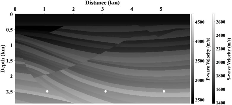
FIGURE 1. Quasi Sigsbee2A model. The structure of the P- and S-wave velocity models is identical.

The migration results of iteration 40th for the quasi-Sigsbee2A model are shown in Figure 2. To demonstrate the accuracy of DELSRTM, the DELSRTM image reflectivity profiles are compared with the real reflectivity in a single trace (Figure 3), which located at the distance of 3090 m and cross the middle diffraction point. Compared with true PP and PS reflectivity, we found that without the help of filtering process, the PP- and PS-image generated by our DELSRTM clearly reconstructed the reflectivity distribution and all the high-speed diffraction points converged perfectly.

FIGURE 2

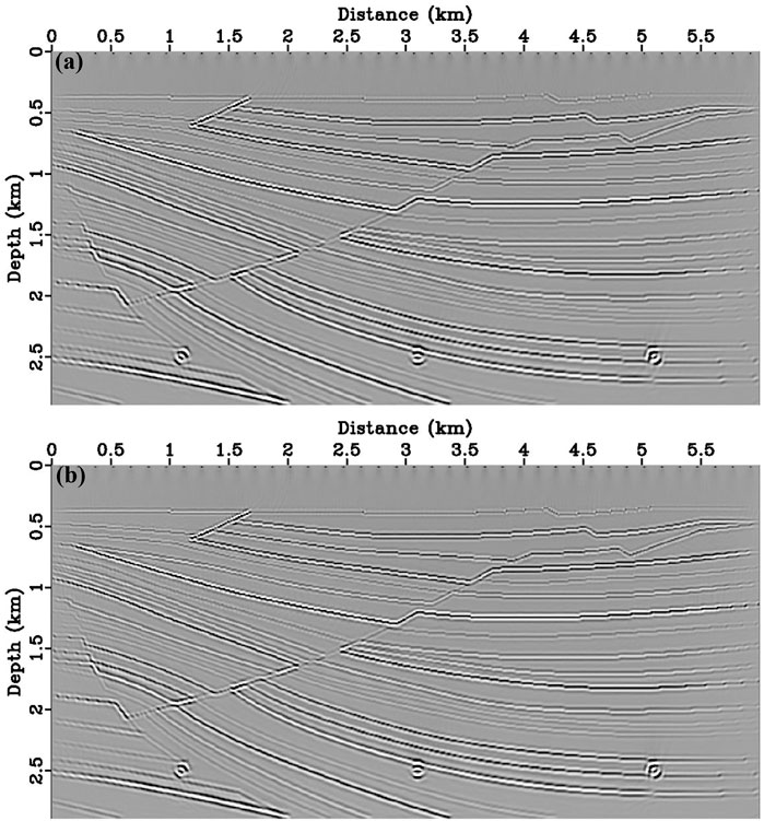
FIGURE 2. Migration results for the Quasi Sigsbee2A model. The true (A) PP and (B) PS reflectivity distribution without filtering processed.

FIGURE 3

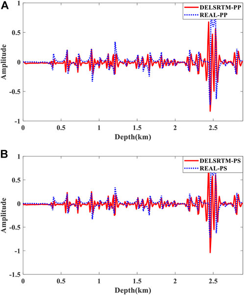
FIGURE 3. For the quasi-Sigsbee2A model, the DELSRTM image reflectivity profiles are compared with the real reflectivity in a single trace at 3090 m. (A) for PP comparison, (B) for PS comparison, the dashed blue lines and solid red lines indicate real and DELSRTM reflectivity, respectively.

3.2 Modified Marmousi2 model

To further verify the anti-crosstalk effect of the DELSRTM, we tested our algorithm using a modified marmousi2 model (Figure 4) with uncorrelated P- and S-wave velocity structures. Moreover, the density is set to be constant (1.0kg/m3). This model is discrete into a grid of 233(z) by 662(x) with a spatial sampling interval of 20 m in both directions. We deployed 30 P-wave sources and 662 receivers, which were uniformly deployed along the surface with 440 and 20 m apart. We used Ricker wavelet with a peak frequency of 40 Hz as the source signature, and the total recording time is 2s, with a sample interval of 0.5 ms. To simulate the propagation of seismic waves numerically in time domain, we used the high-order staggered grid finite-difference (FD) scheme to solve the elastic wave equation with a 5 m by 5 m discrete spatial grid size. Before imaging, we only removed the direct wave to ensure that the DELSRTM gradient is not contaminated by low wave components.

FIGURE 4

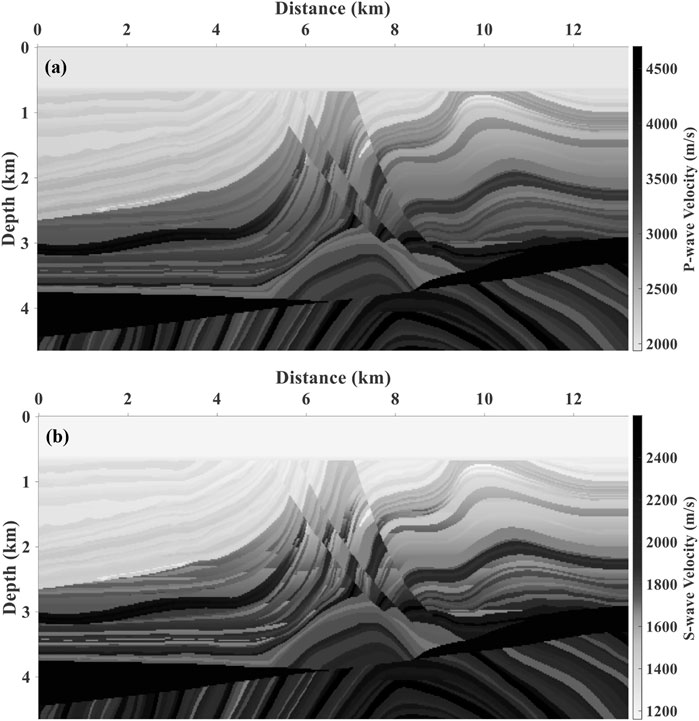
FIGURE 4. Modified marmousi2 model with uncorrelated (A) P- and (B) S-wave velocity models

Figure 6 shows the migration results after forty iterations performed. There are a few low wave-number artifacts in the imaging results since the residual diving waves. The energy of artifacts suppressed some of the weak reflectivity imaging, however, a low-cut filtering process can also annihilate weak reflectivity imaging, which is why we chose not to do high-pass filtering. Compared with the true reflectivity distribution (Figure 5), migration results for the modified marmousi2 model (Figure 6) imaging complex structures accurately, and according to the comparison of single trace which is located at the distance of 5790 m in Figure 7, the proposed DELSRTM reflectivity imaging results are close to the real one. Besides, these yellow boxes in Figure 6 marked imaging results of where P- and S-wave velocity models are uncorrelated. There are few crosstalk artifacts in the image of the marked structures. From what has been discussed above, the P- and S-waves crosstalk artifacts are suppressed in our new DELSRTM scheme when applied to complex and uncorrelated elastic structures.

FIGURE 5

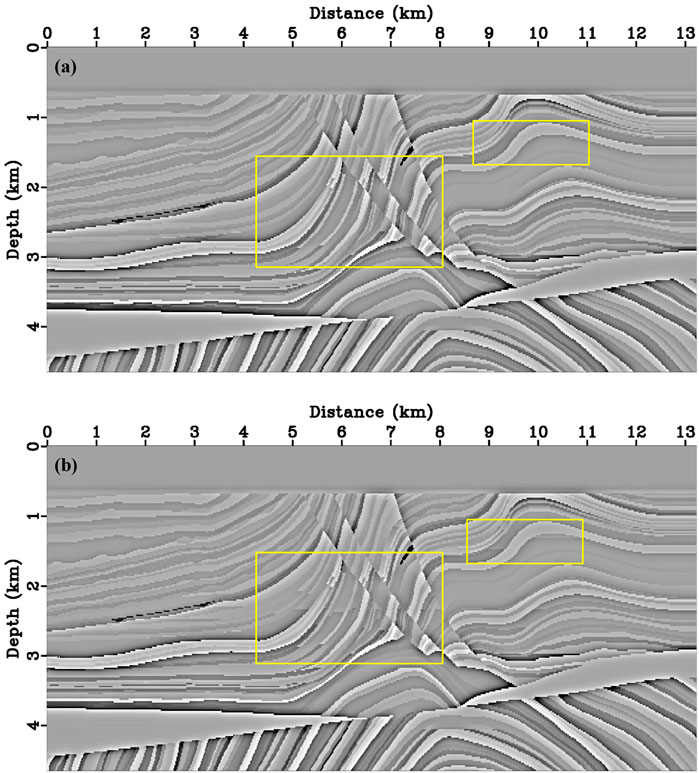
FIGURE 5. The true (A) PP and (B) PS reflectivity distribution of the Modified Marmousi2 model in our numerical test. The reflectivity distribution of uncorrelated P and S-wave velocity structures is indicated by yellow boxes.

FIGURE 6

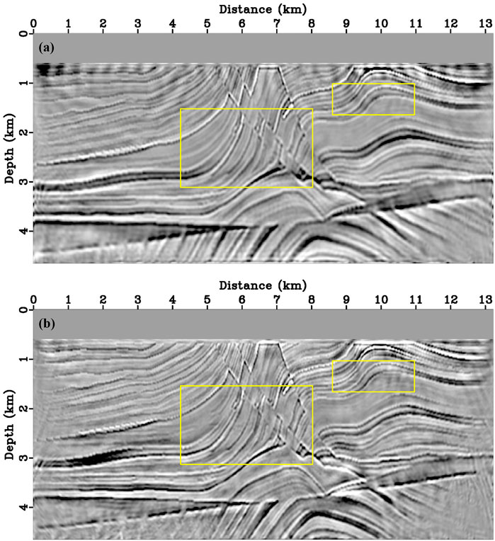
FIGURE 6. Migration results for the modified marmousi2 model. No filtering processed (A) PP- and (B) PS-image which generated from proposed DELSRTM after 40 times iteration. The images of uncorrelated P and S-wave velocity structures are indicated by yellow boxes.

FIGURE 7

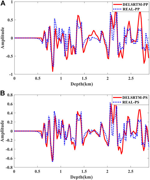
FIGURE 7. For the modified Marmousi2 model, the DELSRTM image reflectivity profiles compared with the real reflectivity in a single trace at 5340 m. (A) for PP comparison, (B) for PS comparison, the dashed blue lines and solid red lines indicate real and DELSRTM reflectivity, respectively.

4 Conclusion

We propose a new scheme of decomposed wavefield least-squares reverse time migration, which effectively suppressed the P- and S-waves crosstalk artifacts. Since the first-order particle velocity-stress equation is not self-adjoint, we adopt a compound strategy to ensure that our algorithm is robust. In the processing of source wavefields vector decomposition, we transform the advantages of wavenumber domain-based wavefields vector decomposition method into time-space domain and improve the computational efficiency with minimal computational cost. Different from the method of source wavefields vector decomposition, in the process of adjoint-wavefield decomposition, we construct the shear component which is subtracted to separate P- and S- waves mode. The gradient of the decomposed wavefield least-squares reverse time migration was calculated using the separated P- and S-waves wavefields on both sides, and crosstalk-less gradients guarantee the accuracy of reflectivity imaging. Unlike ELSRTM, which is based on the decoupled wave equation method, our scheme produces correct results even when the P- and S-wave velocity models are uncorrelated and change dramatically. In addition, the physical significance of our new wavefield-decomposed ELSRTM scheme is clear.

Data availability statement

The raw data supporting the conclusions of this article will be made available by the authors, without undue reservation.

Author contributions

WL contributed to the conception and design of the study. QD modified the manuscript. All authors contributed to manuscript revision and read and approved the submitted version.

Funding

This research is supported by the Key Project of National Natural Science Foundation of China (41930429) and 14th 5-Year Prospective and Basic Research Program of CNPC (2021DJ3506).

Acknowledgments

We are grateful to editor LD and reviewers QL, XG, and KY for reviewing this manuscript.

Conflict of interest

Authors JZ and ZZ were employed by the R&D Center, Bureau of Geophysical Prospecting Inc.

The remaining authors declare that the research was conducted in the absence of any commercial or financial relationships that could be construed as a potential conflict of interest.

Publisher’s note

All claims expressed in this article are solely those of the authors and do not necessarily represent those of their affiliated organizations, or those of the publisher, the editors and the reviewers. Any product that may be evaluated in this article, or claim that may be made by its manufacturer, is not guaranteed or endorsed by the publisher.

References

Baysal, E., Kosloff, D., and Sherwood, J. (1983). Reverse time migration. Geophysics 48, 1514–1524. doi:10.1190/1.1441434

CrossRef Full Text | Google Scholar

Dai, W., and Schuster, G. T. (2013). Plane-wave least-squares reverse-time migration. Geophysics 78 (4), S165–S177. doi:10.1190/geo2012-0377.1

CrossRef Full Text | Google Scholar

Dellinger, J., and Etgen, J. (1990). Wave-field separation in two-dimensional anisotropic media. Geophysics 55 (7), 914–919. doi:10.1190/1.1442906

CrossRef Full Text | Google Scholar

Dong, S., Cai, J., Guo, M., Suh, S., Zhang, Z., Wang, B., et al. (2012). Least- squares reverse time migration: Towards true amplitude imaging and improving the resolution. 82nd Annual International Meeting, SEG, Expanded Abstracts, Las Vegas, NV, November 2012. doi:10.1190/segam2012-1488.1

CrossRef Full Text | Google Scholar

Du, Q. Z., Guo, C., Zhao, Q., Gong, X., Wang, C., and Li, X. (2017). Vector- based elastic reverse time migration based on scalar imaging condition. Geophysics 82, S111–S127. doi:10.1190/geo2016-0146.1

CrossRef Full Text | Google Scholar

Du, Q. Z., Zhang, M. Q., Chen, X. R., Gong, X. F., and Guo, C. F. (2014). True-amplitude wavefield separation using staggered-grid interpolation in the wavenumber domain. Appl. Geophys. 11 (4), 437–446. doi:10.1007/s11770-014-0458-9

CrossRef Full Text | Google Scholar

Du, Q. Z., Zhu, Y. T., and Ba, J. (2012). Polarity reversal correction for elastic reverse time migration. Geophysics 77 (2), S31–S41. doi:10.1190/geo2011-0348.1

CrossRef Full Text | Google Scholar

Duan, Y., and Sava, P. (2015). Scalar imaging condition for elastic reverse time migration. Geophysics 80 (4), S127–S136. doi:10.1190/geo2014-0453.1

CrossRef Full Text | Google Scholar

Feng, Z. C., and Schuster, G. T. (2017). Elastic least-squares reverse time migration. Geophysics 82, S143–S157. doi:10.1190/segam2016-13863861.1

CrossRef Full Text | Google Scholar

Gong, X. F., Du, Q. Z., and Zhao, Q. (2018). SP- and SS-imaging for 3D elastic reverse time migration. Geophysics 83 (1), A1–A6. doi:10.1190/geo2017-0286.1

CrossRef Full Text | Google Scholar

Gu, B., Li, Z., and Han, J. (2018). A wavefield-separation-based elastic least-squares reverse time migration. Geophysics 83 (3), S279–S297. doi:10.1190/geo2017-0131.1

CrossRef Full Text | Google Scholar

Hemon, C. (1978). Equations d’onde et modeles. Geophys. Prospect. 26, 790–821. doi:10.1111/j.1365-2478.1978.tb01634.x

CrossRef Full Text | Google Scholar

LeBras, R., and Clayton, W. (1988). An iterative inversion of back‐scattered acoustic waves. Geophysics 53 (4), 501–508. doi:10.1190/1.1442481

CrossRef Full Text | Google Scholar

Li, Z., Zhang, H., Liu, Q., and Han, W. (2007). Numeric simulation of elastic wavefield separation by staggering grid high-order finite-difference algorithm. Oil Geophys. Prospect. 42 (5), 510–515. doi:10.3321/j.issn:1000-7210.2007.05.006

CrossRef Full Text | Google Scholar

Liu, B., Wang, J. S., Ren, Y. X., Guo, X., Chen, L., and Liu, L. B. (2022). Decoupled elastic least-squares reverse time migration and its application in tunnel geologic forward prospecting. Geophysics 87, EN1–EN19. doi:10.1190/geo2020-0875.1

CrossRef Full Text | Google Scholar

Liu, Q., and Peter, D. (2018). One-step data-domain least-squares reverse time migration. Geophysics 83 (4), R361–R368. doi:10.1190/geo2017-0622.1

CrossRef Full Text | Google Scholar

Liu, Q., and Tromp, J. (2006). Finite-frequency kernels based on adjoint methods. Bull. Seismol. Soc. Am. 96 (6), 2383–2397. doi:10.1785/0120060041

CrossRef Full Text | Google Scholar

Ma, D., and Zhu, G. (2003). P- and S-wave separated elastic wave equation numerical modeling. Oil Geophys. Prospect. 38, 482–486. doi:10.3321/j.issn:1000-7210.2007.05.006

CrossRef Full Text | Google Scholar

McMechan, G. (1983). Migration by extrapolation of time-dependent boundary values. Geophys. Prospect. 31, 413–420. doi:10.1111/j.1365-2478.1983.tb01060.x

CrossRef Full Text | Google Scholar

Nemeth, T., Wu, C., and Schuster, G. T. (1999). Least-squares migration of incomplete reflection data. Geophysics 64 (1), 208–221. doi:10.1190/1.1444517

CrossRef Full Text | Google Scholar

Plessix, R. -E. (2006). A review of the adjoint-state method for computing the gradient of a functional with geophysical applications. Geophys. J. Int. 167 (2), 495–503. doi:10.1111/j.1365-246X.2006.02978.x

CrossRef Full Text | Google Scholar

Qu, Y., Li, J., Huang, J., and Li, Z. (2018). Elastic least-squares reverse time migration with velocities and density perturbation. Geophys. J. Int. 212 (2), 1033–1056. doi:10.1093/gji/ggx468

CrossRef Full Text | Google Scholar

Ren, Z., and Liu, Y. (2015). Elastic full-waveform inversion using the second- generation wavelet and an adaptive-operator-length scheme. Geophysics 80 (4), R155–R173. doi:10.1190/geo2014-0516.1

CrossRef Full Text | Google Scholar

Ren, Z., Liu, Y., and Sen, M. K. (2017). Least-squares reverse time migration in elastic media. Geophys. J. Int. 208 (2), 1103–1125. doi:10.1093/gji/ggw443

CrossRef Full Text | Google Scholar

Ren, Z. M., and Liu, Y. (2016). A hierarchical elastic full-waveform inversion scheme based on wavefield separation and the multistep-length approach. Geophysics 81 (3), R99–R123. doi:10.1190/geo2015-0431.1

CrossRef Full Text | Google Scholar

Schuster, G. T. (1993). Least-squares cross-well migration. 63rd Annual International Meeting, SEG, Expanded Abstracts, Washington, DC, September 1993, 110–113. doi:10.1190/1.1822308

CrossRef Full Text | Google Scholar

Sears, T. J., Barton, P. J., and Singh, S. C. (2010). Elastic full waveform inversion of multicomponent ocean-bottom cable seismic data: Application to Alba field, U.K. North Sea. Geophysics 75 (6), R109–R119. doi:10.1190/1.3484097

CrossRef Full Text | Google Scholar

Shi, Y., Li, S., and Zhang, W. (2021). Prestack correlative elastic least-squares reverse time migration based on wavefield decomposition. J. Appl. Geophys., 194, 104447. doi.org/doi:10.1016/j.jappgeo.2021.104447

CrossRef Full Text | Google Scholar

Sun, R., and McMechan, G. A. (2001). Scalar reverse-time depth migration of prestack elastic seismic data. Geophysics 66, 1519–1527. doi:10.1190/1.1487098

CrossRef Full Text | Google Scholar

Virieux, J. (1986). P-SV wave propagation in heterogeneous media: Velocity-stress finite-difference method. Geophysics 51 (4), 889–901. doi:10.1190/1.1442147

CrossRef Full Text | Google Scholar

Wang, W., and McMechan, G. A. (2015). Vector-based elastic reverse time migration. Geophysics 80 (6), S245–S258. doi:10.1190/geo2014-0620.1

CrossRef Full Text | Google Scholar

Whitmore, D. (1983). Iterative depth migration by backward time propagation. SEG Technical Program Expanded Abstracts, Las Vegas, NV, September 1983 382–385. doi:10.1190/1.1893867

CrossRef Full Text | Google Scholar

Xiao, X., and Leaney, W. S. (2010). Local vertical seismic profiling (VSP) elastic reverse-time migration and migration resolution: Salt-flank imaging with transmitted P-to-S waves. Geophysics 75 (2), S35–S49. doi:10.1190/1.3309460

CrossRef Full Text | Google Scholar

Yan, J., and Sava, P. (2008). Isotropic angle-domain elastic reverse-time migration. Geophysics 73 (6), S229–S239. doi:10.1190/1.2981241

CrossRef Full Text | Google Scholar

Yang, J. D., Zhu, H. J., McMechan, G., Zhang, H. Z., and Zhao, Y. (2019). Elastic least-squares reverse time migration in vertical transverse isotropic media. Geophysics 84 (6), S539–S553. doi:10.1190/geo2018-0887.1

CrossRef Full Text | Google Scholar

Yao, G., and Jakubowicz, H. (2012). Least-squares reverse-time migration. SEG Technical Program Expanded Abstracts, Las Vegas, NV, November 2012, 1–5. doi:10.1190/segam2012-1425.1

CrossRef Full Text | Google Scholar

Zhang, J., Tian, Z., and Wang, C. (2007). P-and S-wave separated elastic wave equation numerical modeling using 2D staggered-grid. SEG Technical Program Expanded Abstracts, San Antonio, TX, United States, September 2007, 2014–2019. doi:10.1190/1.2792904

CrossRef Full Text | Google Scholar

Zhang, Q. S., and McMechan, A. G. (2010). 2D and 3D elastic wavefield vector decomposition in the wavenumber domain for VTI media. Geophysics 75, D13–D26. doi:10.1190/1.3431045

CrossRef Full Text | Google Scholar

Zhang, W., and Gao, J. (2022). Attenuation compensation for wavefield-separation-based least-squares reverse time migration in viscoelastic media. Geophys. Prospect., 70(2), 280–317. doi.org/doi:10.1111/1365-2478.13161

CrossRef Full Text | Google Scholar

Zhang, W., Gao, J., Gao, Z., and Shi, Y. (2020), 2D and 3D amplitude-preserving elastic reverse time migration based on the vector-decomposed P- and S-wave records. Geophys. Prospect., 68(9), 2712–2737. doi.org/doi:10.1111/1365-2478.13023

CrossRef Full Text | Google Scholar

Zhang, Y., Duan, L., and Xie, Y. (2013). A stable and practical implementation of least-squares reverse time migration. SEG Technical Program Expanded Abstracts, Houston, TX, September 2013, 3716–3720. doi:10.1190/segam2013-0577.1

CrossRef Full Text | Google Scholar

Zhang, Y., Duan, L., and Xie, Y. (2015). A stable and practical implementation of least-squares reverse time migration. Geophysics 80 (1), V23–V31. doi:10.1190/geo2013-0461.1

CrossRef Full Text | Google Scholar

Zhong, Y., Gu, H. M., Liu, Y. T., and Mao, Q. H. (2021). Elastic least-squares reverse time migration based on decoupled wave equations. Geophysics 86 (6), S371–S386. doi:10.1190/geo2020-0805.1

CrossRef Full Text | Google Scholar

Zhou, X., Chang, X., Wang, Y., and Yao, Z. (2018). Scalar PP and PS imaging of elastic RTM by wavefield decoupling method. SEG Technical Program Expanded Abstracts, Anaheim, CA, October 2018, 2417–2421. doi:10.1190/segam2018-2995359.1

CrossRef Full Text | Google Scholar