- School of Geosciences, China University of Petroleum (East China), Qingdao, Shandong, China
Reservoir parameter prediction is of significant value to oil and gas exploration and development. Artificial intelligence models are developing rapidly in reservoir parameter prediction. Unfortunately, current research has focused on multi-input single-output prediction models. Meaning, these models use a large amount of logging or seismic data to predict the petrophysical properties of a single reservoir. Another prominent problem is that most mechanistic learning studies have focused on using logging data (e.g., gamma ray and resistivity) to make predictions of reservoir parameters. Although these studies have yielded promising accuracy, a great shortcoming is the inability to obtain such data in logs by seismic inversion. The value of our research work is to achieve a complete description of the reservoir using the elastic parameters from the seismic inversion. We developed a deep learning method based on gated recurrent neural network (GRNN) suitable for simultaneous prediction of porosity, saturation and shale content in the reservoir. GRNN is based on Gated Recurrent Unit (GRU), which can automatically update and reset the hidden state. The input parameters to the model are compressive wave velocity, shear wave velocity and density. The model is trained to fit nonlinear relationships between input parameters and multiple physical parameters. We employed two wells: one for testing and the other for training. 20% of the data in the training wells were used as the validation set. In preprocessing, we performed z-score whitening on the input data. During the training phase, the model hyperparameters were optimized based on the mean absolute error (MAE) box plots of the validation set. Experiments on the test data show that the model has superior robustness and accuracy compared to the conventional recurrent neural network (RNN). In the GRNN prediction results of the test set, the MAE is 0.4889 and the mean squared error (MSE) is 0.5283. Due to the difference in input parameters, our prediction is weaker than the research method using logging data. However, our proposed method has higher practical value in exploration work.
Introduction
Prediction and analysis of porosity, water saturation, and shale content in reservoir delineation, geological modelling and well location distribution play an important role in reservoir delineation, geological modelling and well location distribution in the process of oil exploration and development (Eberhart-Phillips et al., 1989; Pang et al., 2019). These reservoir parameters are generally derived from logging data or core data (Segesman, 1980). However, the physical parameters in logging cannot characterize the distribution of reservoir parameters in unknown intervals or the entire work area, and are subject to cost constraints (Gyllensten et al., 2004). Therefore, empirical formulas or models are needed to calculate and predict (Goldberg and Gurevich, 2008). Due to the complex conditions of geology, logging data often exhibit strong nonlinear relationships between them, and this nonlinear relationship may never be exactly obtained at the theoretical level (Ballin et al., 1992). Traditional forecasting methods have their own limitations for accurate prediction of reservoir parameters (Hamada, 2004; Chatterjee et al., 2013). The effects of longitudinal and transverse velocities on porosity and shale content are thought to have some correlation, but are difficult to predict quantitatively (Han et al., 1986). Continuous sound velocity logging methods can only qualitatively identify water-saturated rock masses (Hicks and Berry, 1956). Laboratories can measure high-quality physical properties, but at an additional time and cost (Gomez et al., 2010). Therefore, numerical models of the petrophysical properties of the formation need to be established for reservoir characterization from measurable data (Tian et al., 2012). The prediction of the distribution of reservoir quality (i.e., porosity, water saturation, and shale content, etc.) has important implications for estimating the development value of reservoirs (Timur, 1968).
Modern reservoir characterization has evolved from the use of experts to analyze and interpret log data to the application of artificial intelligence to automatically identify predictions (Soleimani et al., 2020). Machine learning methods such as artificial neural network, K-proximity, support vector machine and function network have been widely used in the field of petroleum exploration due to their high efficiency and accuracy. This helps to solve many technical problems such as reservoir identification (Aminian and Ameri, 2005; Wang et al., 2017), reservoir fluid prediction (Oloso et al., 2017; Mahdiani and Norouzi, 2018), permeability prediction (Tahmasebi and Hezarkhani, 2012; Al-Mudhafar, 2019; Al Khalifah et al., 2020) and rock strength and geomechanical properties (Tariq et al., 2016; Tariq et al., 2017). Computer-based machine learning methods can effectively handle nonlinear problems and predict reliable reservoir property values (Kaydani et al., 2011).
Deep learning is an important branch of machine learning, which has gradually become a research hotspot in recent years (Lecun et al., 2015; Guo et al., 2016; Zhang et al., 2020). Research has proved that deep learning techniques are prominent at dealing with complex structures in high-dimensional spaces (Michelucci, 2018), and have been used in image recognition (Shuai et al., 2016), speech recognition (Saon et al., 2021) and language translation (Jean et al., 2014) and have achieved excellent results. In recent years, many scholars have applied it to the field of seismic exploration (Lin et al., 2018; He et al., 2020). For example, reservoir fracture parameter prediction (Xue et al., 2014; Wang et al., 2021; Yasin et al., 2022), lithology identification (Al-Mudhafar, 2020; Alzubaidi et al., 2021; Saporetti et al., 2021) and seismic inversion (Li et al., 2019; Cao et al., 2021), etc.
Classical back-propagation (BP) neural networks have been studied for prediction on well logging data (Al-Bulushi et al., 2012; Verma et al., 2012). Since the data information extracted by neurons is not transmitted in the same hidden layer, fully connected neural network is not suitable for effective prediction of sequence data. For data with sequence information, Recurrent Neural Network (RNN) (Mikolov et al., 2010; Zhang et al., 2017) can learn the relationships and laws within the data and make preferable predictions. RNNs consist of high-dimensional hidden states with nonlinear dynamics (Sutskever et al., 2011).
Among the different variants of RNNs, one that has attracted tremendous attention is the network formed using Gated Recurrent Unit (GRU)—Gated Recurrent Neural Network (GRNN) (Chung et al., 2014). The learning curves of GRNN on many datasets demonstrate significant advantages over standard RNN and are able to avoid the vanishing and exploding gradient problems of standard RNN when dealing with long sequences (Bengio et al., 1994). GRNN has been applied to log parameter prediction and lithology identification (Zeng et al., 2020), and to predict mass production in conglomerate reservoirs (Li et al., 2020). Some scholars have tried to combine GRNN with convolutional neural network to predict porosity (Wang and Cao, 2021).
We have noticed two neglected problems in the research on reservoir physical parameter prediction by mechanical learning. One issue is that the research programs can only predict a single reservoir parameter (Rui et al., 2019; Chen et al., 2020). The other issue is that the investigations are limited to parameters specific to the logs as model inputs (Ahmadi and Chen, 2019; Okon et al., 2021). This means that it is not possible to predict reservoir physical parameters for the whole work area and lacks practical value.
In this paper, the GRU-based GRNN model is used to simultaneously predict the physical parameters of the logging data. The structure and principle of GRU are analyzed, and a prediction model is founded by using the nonlinear relationship between elastic parameters [compressive wave velocity (
Methods
Figure 1 depicts the study’s workflow. We first normalize the model’s input data. Well B is utilized to test the model’s generalizability while Well A is used as training data. Create a GRNN model fit for regression tasks, then tune the hyperparameters. The trained model is used to predict the physical properties of the reservoir after being tested in Well B.
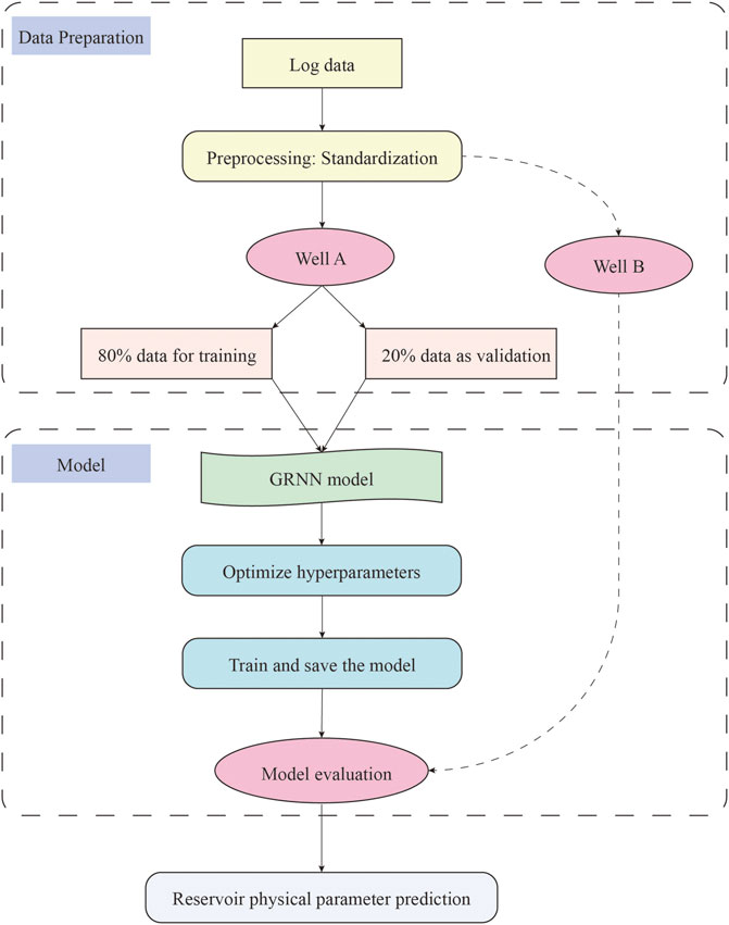
FIGURE 1. Workflow. The log data is separated into training, validation, and test sets after being standardized. GRNN model construction and hyperparameter optimization. Test model generalization and predict reservoir physical properties.
RNN
Before introducing GRU, we need to introduce the classic RNN. RNN is a neural network with a hidden state and an output sequence, as shown in Figure 2. The input to the network is a variable-length sequence
where

FIGURE 2. RNN structure. Each structural unit accepts both the input data and the hidden state of the previous unit, and outputs the predicted value at the current moment.
The RNN learns the probability distribution
where
By iterative sampling at each time step,
GRU
Figure 3 describes the specific structure of the GRU. GRU has two important gating units—reset gate and update gate. In the
where
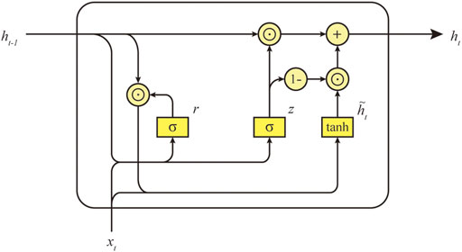
FIGURE 3. Compute the hidden state of the GRU model. Update gate
The calculation method for the update gate
The final hidden state
where
where
The update gate controls the ratio of previous hidden states to candidate hidden states. When the update gate
GRNN uses GRU to adjust the information transfer in RNN, so that the sequence model can retain effective information for a long time, forget irrelevant information, and effectively avoid the problems of gradient disappearance and explosion. In this research, GRNN is used to predict reservoir physical parameters. Logging parameters can be regarded as sequence information. The ability of GRNN to explore effective information adaptively is more suitable for the task of reservoir parameter prediction.
Data description and model
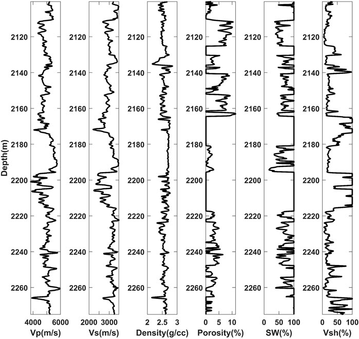
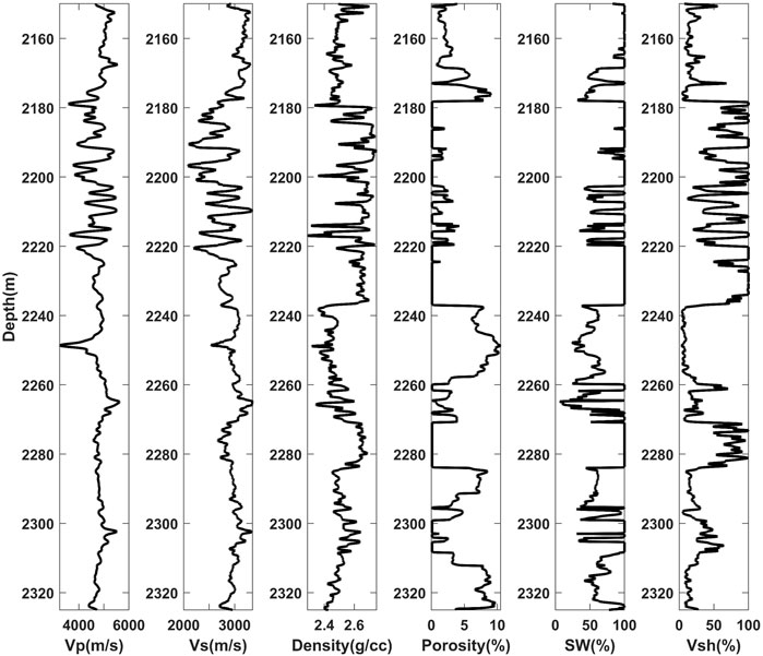
The experimental data we utilize are from the work area of the sandstone reservoir. The datasets used to predict reservoirs
Before model training, to ensure that the model can effectively adjust the weights and biases, we normalize the data with z-score (mean 0, variance 1):
where
Establish GRNN model
In this study, we used Python version 3.7.0 to implement the model via the Tensorflow platform.
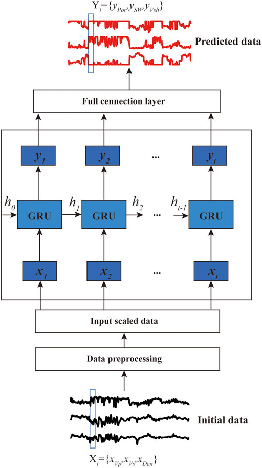
Figure 6 presents the design framework of the GRNN model. The input data of the model is
Compared with the classical BP neural network, GRNN is preferable at mining the information between sequences. And due to the structure of GRU, GRNN can filter unimportant information to a certain extent, retain the characteristic information of logging data, and improve the prediction accuracy of physical parameters.
Result and discussion
Fitting and generalization
When a model is trained, if it performs well on the training set but cannot predict accurately on the new test set data, then the model has no real value. In machine learning, this type of problem is called overfitting (Ying, 2019). However, if there is not enough data or the complexity of the model is lower than that required for fitting, the model cannot predict accurately even on the training set and is equally useless. This type of problem is called underfitting (Jabbar and Khan, 2015). In the case of supervised learning, whether it is overfitting or underfitting, it is necessary to pay attention to avoid it when debugging the model.
Generalization ability is very important for any machine learning model. We are always interested in how well a model predicts unknown data, because this can reflect the practical value of the model. Therefore, all evaluation indicators are subject to test data. Among the techniques for overfitting, a common method is dropout (Mianjy and Arora, 2020), i.e., randomly turning off neurons at a certain ratio (between 0 and 1) during each iteration. In the GRNN network, the Dropout value can be set in the hidden layer.
Parameter setting
We use well A logging data to train the model and analyze the effect of different parameter settings on the results. Three network parameters of GRNN are selected: learning rate (
We train the model with different hyperparameters and choose mean absolute error (MAE) and mean squared error (MSE) as metrics:
where
Boxplots are drawn based on the prediction error on the validation set, as shown in Figure 7. Boxplots show 75% and 25% quantiles, medians, outliers, maximum and minimum values. It can be seen that outliers will exist in most cases. Outliers may come from the initial stage of training when the model fitting ability is inferior, and there is a large gap between the predicted value and the true value. The optimal hyperparameters chosen based on the smallest median are
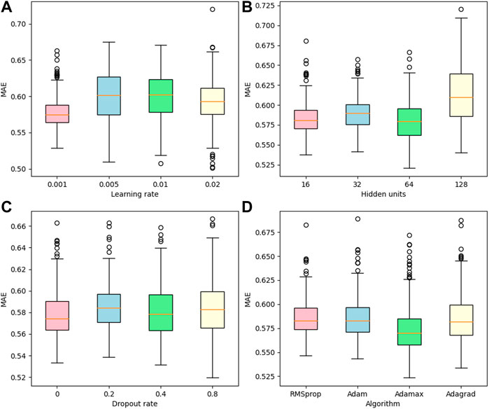
FIGURE 7. Box plot. The model is trained using the well A data, and the network hyperparameters are adjusted according to the MAE values of the validation set. (A) learning rate, (B) hidden units, (C) dropout rate, (D) algorithm.
Comparison with RNN
To evaluate the accuracy of the GRNN model for simultaneously predicting
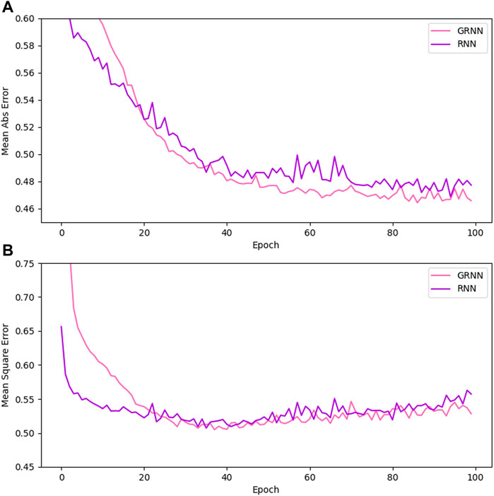
FIGURE 8. Comparison of prediction errors of GRNN and RNN for well B during iteration. (A) MAE, (B) MSE.
Fitting and prediction of logging data
We use the trained GRNN model to predict Well A and observe the effect of the model fitting the training set, as shown in Figure 9. For the prediction results of
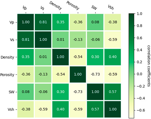
Figure 10 presents the PPMCC matrix calculated from Well A data. PPMCC helps analyze the degree of correlation between variables. The closer the coefficient is to 1, the stronger the positive correlation between the two variables. Conversely, if the coefficient is closer to −1, it indicates that the two variables are more negatively correlated. When the coefficient is close to 0, it is considered that there is little connection between the variables. As shown by the figure, the correlation coefficients of
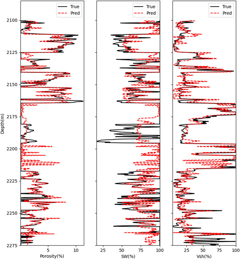
Finally, we present the prediction results for the test set well B, as shown in Figure 11. The predicted results for
Prediction of reservoir physical parameters
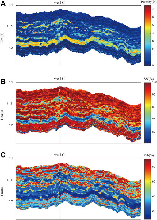
Through the inversion method, we obtained the elastic parameters of the actual work area, as shown in Figure 12. Figures 12A–C are the compressional wave velocity, shear wave velocity and density of the reservoir, respectively. We use the trained GRNN model to predict the physical parameters of the actual working area, as shown in Figure 13. Figures 13A–C are the prediction results of

FIGURE 12. Reservoir elastic parameters from inversion. (A) P-wave velocity, (B) S-wave velocity, (C) density.
Conclusion
The prediction of physical parameters such as porosity, permeability, and saturation is an important work in reservoir prediction. Nowadays, many scholars try to apply deep learning to physical property prediction. However, most of the current work is to use the electrical parameters with high correlation to predict the logging parameters instead of the elastic parameters that can be obtained in the actual work area, and only use various models to predict a single parameter. This lacks application value for reservoir prediction.
This paper describes how to apply the GRNN model to the simultaneous prediction of reservoir physical parameters (porosity, water saturation, and shale content). GRNN is a special recurrent neural network that enables sequence information to be transmitted between the same hidden layers. The structure of the gate control unit enables it to store and forget information, and realize the extraction and control of information flow. GRNN can simultaneously predict physical parameters using longitudinal wave velocity, shear wave velocity and density, and the prediction error is smaller than that of RNN. The model predicts well B in the test set with an average MAE and an average MSE of 0.4889 and 0.5293, respectively. The Pearson product moment correlation coefficients of the elastic parameters and physical parameters used in the model are calculated, and the results show that the correlation between the elastic parameters and the physical parameters is not high. In particular, water saturation has almost only a positive correlation with density. Nonetheless, the models can still fit their nonlinear relationship in high dimensions. The GRNN model can also predict and reconstruct the missing sections of the log. In future work, attempts will be made to change the structure of the network as well as the properties of the input data to improve the prediction accuracy. The prediction of various physical property parameters of reservoirs has guiding significance for oil and gas exploration. The application of elastic parameters to achieve physical property prediction has general value for actual exploration work in different work areas.
Our suggested method for predicting reservoir parameters still has several limitations. The accuracy of the seismic inversion decides the effectiveness of the prediction. A local optimum rather than a global optimum may be the result of model training.
Data availability statement
The original contributions presented in the study are included in the article/supplementary material, further inquiries can be directed to the corresponding author.
Author contributions
JZ: Conceptualization, methodology, writing-original draft preparation. ZL: Supervision, software. GZ: Validation, investigation. BY: Visualization. XN: Data curation. TX: Writing-Reviewing and editing.
Conflict of interest
The authors declare that the research was conducted in the absence of any commercial or financial relationships that could be construed as a potential conflict of interest.
Publisher’s note
All claims expressed in this article are solely those of the authors and do not necessarily represent those of their affiliated organizations, or those of the publisher, the editors and the reviewers. Any product that may be evaluated in this article, or claim that may be made by its manufacturer, is not guaranteed or endorsed by the publisher.
References
Ahmadi, M. A., and Chen, Z. (2019). Comparison of machine learning methods for estimating permeability and porosity of oil reservoirs via petro-physical logs. Petroleum 5 (3), 271–284. doi:10.1016/j.petlm.2018.06.002
Al Khalifah, H., Glover, P., and Lorinczi, P. (2020). Permeability prediction and diagenesis in tight carbonates using machine learning techniques. Mar. Pet. Geol. 112, 104096. doi:10.1016/j.marpetgeo.2019.104096
Al-Bulushi, N. I., King, P. R., Blunt, M. J., and Kraaijveld, M. (2012). Artificial neural networks workflow and its application in the petroleum industry. Neural comput. Appl. 21 (3), 409–421. doi:10.1007/s00521-010-0501-6
Al-Mudhafar, W. J. (2019). Bayesian and LASSO regressions for comparative permeability modeling of sandstone reservoirs. Nat. Resour. Res. 28 (1), 47–62. doi:10.1007/s11053-018-9370-y
Al-Mudhafar, W. J. (2020). Integrating machine learning and data analytics for geostatistical characterization of clastic reservoirs. J. Pet. Sci. Eng. 195, 107837. doi:10.1016/j.petrol.2020.107837
Alzubaidi, F., Mostaghimi, P., Swietojanski, P., Clark, S. R., and Armstrong, R. T. (2021). Automated lithology classification from drill core images using convolutional neural networks. J. Pet. Sci. Eng. 197, 107933. doi:10.1016/j.petrol.2020.107933
Aminian, K., and Ameri, S. (2005). Application of artificial neural networks for reservoir characterization with limited data. J. Pet. Sci. Eng. 49 (3-4), 212–222. doi:10.1016/j.petrol.2005.05.007
Ballin, P. R., Journel, A. G., and Aziz, K. (1992). Prediction of uncertainty in reservoir performance forecast. J. Can. Petroleum Technol. 31 (04). doi:10.2118/92-04-05
Bengio, Y., Simard, P., and Frasconi, P. (1994). Learning long-term dependencies with gradient descent is difficult. IEEE Trans. Neural Netw. 5 (2), 157–166. doi:10.1109/72.279181
Bock, S., and Weiß, M. (2019). “A proof of local convergence for the Adam optimizer,” in 2019 International Joint Conference on Neural Networks (IJCNN) (Budapest, Hungary: IEEE), 1–8.
Cao, D., Su, Y., and Cui, R. (2021). Multi-parameter pre-stack seismic inversion based on deep learning with sparse reflection coefficient constraints. J. Pet. Sci. Eng. 209, 109836. doi:10.1016/j.petrol.2021.109836
Chatterjee, R., Gupta, S. D., and Farroqui, M. Y. (2013). Reservoir identification using full stack seismic inversion technique: A case study from cambay basin oilfields, India. J. Pet. Sci. Eng. 109, 87–95. doi:10.1016/j.petrol.2013.08.006
Chen, W., Yang, L., Zha, B., Zhang, M., and Chen, Y. (2020). Deep learning reservoir porosity prediction based on multilayer long short-term memory network. Geophysics 85 (4), WA213–WA225. doi:10.1190/geo2019-0261.1
Chung, J., Gulcehre, C., Cho, K., and Bengio, Y. (2014). Empirical evaluation of gated recurrent neural networks on sequence modeling. Comput. Sci., Neu. Evolut. Comput.. arXiv:1412.3555.
Duchi, J., Hazan, E., and Singer, Y. (2011). Adaptive subgradient methods for online learning and stochastic optimization. J. Mach. Learn. Res. 12 (7), 2121–2159. doi:10.5555/1953048.2021068
Eberhart-Phillips, D., Han, D., and Zoback, M. D. (1989). Empirical relationships among seismic velocity, effective pressure, porosity, and clay content in sandstone. Geophysics 54 (1), 82–89. doi:10.1190/1.1442580
Emerson, R. W. (2015). Causation and Pearson's correlation coefficient. J. Vis. Impair. Blind. 109 (3), 242–244. doi:10.1177/0145482x1510900311
Goldberg, I., and Gurevich, B. (2008). A semi-empirical velocity-porosity-clay model for petrophysical interpretation of P- and S-velocities. Geophys. Prospect. 46 (3), 271–285. doi:10.1046/j.1365-2478.1998.00095.x
Gomez, C. T., Dvorkin, J., and Vanorio, T. (2010). Laboratory measurements of porosity, permeability, resistivity, and velocity on Fontainebleau sandstones. Geophysics 75 (6), E191–E204. doi:10.1190/1.3493633
Graves, A. (2012). “Long short-term memory,” in Supervised sequence labelling with recurrent neural networks (Berlin, Heidelberg: Springer), 37–45.
Guo, Y., Liu, Y., Oerlemans, A., Lao, S., Wu, S., and Lew, M. S. (2016). Deep learning for visual understanding: A review. Neurocomputing 187, 27–48. doi:10.1016/j.neucom.2015.09.116
Gyllensten, A., Tilke, P., Al-Raisi, M., and Allen, D. (2004). “Porosity heterogeneity analysis using geostatistics,” in Abu dhabi international conference and exhibition (OnePetro).
Hamada, G. M. (2004). Reservoir fluids identification using Vp/Vs ratio? Oil Gas Sci. Technol. -. Rev. IFP. 59 (6), 649–654. doi:10.2516/ogst:2004046
Han, D., Nur, A., and Morgan, D. (1986). Effects of porosity and clay content on wave velocities in sandstones. Geophysics 51 (11), 2093–2107. doi:10.1190/1.1442062
He, M., Gu, H., and Wan, H. (2020). Log interpretation for lithology and fluid identification using deep neural network combined with MAHAKIL in a tight sandstone reservoir. J. Pet. Sci. Eng. 194, 107498. doi:10.1016/j.petrol.2020.107498
Hicks, W. G., and Berry, J. E. (1956). Application of continuous velocity logs to determination of fluid saturation of reservoir rocks. Geophysics 21 (3), 739–754. doi:10.1190/1.1438267
Jabbar, H., and Khan, R. Z. (2015). “Methods to avoid over-fitting and under-fitting in supervised machine learning (comparative study),” in Computer science, communication and instrumentation devices, 70. doi:10.3850/978-981-09-5247-1_017
Jean, S., Cho, K., Memisevic, R., and Bengio, Y. (2014). On using very large target vocabulary for neural machine translation Comput. Sci., Neu. Evolut. Comput.. arXiv:1412.2007.
Kaydani, H., Mohebbi, A., and Baghaie, A. (2011). Permeability prediction based on reservoir zonation by a hybrid neural genetic algorithm in one of the Iranian heterogeneous oil reservoirs. J. Pet. Sci. Eng. 78 (2), 497–504. doi:10.1016/j.petrol.2011.07.017
Kingma, D. P., and Ba, J. (2014). Adam: A method for stochastic optimization Comput. Sci., Neu. Evolut. Comput.. arXiv:1412.6980.
Lecun, Y., Bengio, Y., and Hinton, G. (2015). Deep learning. Nature 521 (7553), 436–444. doi:10.1038/nature14539
Li, S., Liu, B., Ren, Y., Chen, Y., Yang, S., Wang, Y., et al. (2019). Deep-learning inversion of seismic data Comput. Sci., Neu. Evolut. Comput.. arXiv:1901.07733.
Li, X., Ma, X., Xiao, F., Wang, F., and Zhang, S. (2020). Application of gated recurrent unit (GRU) neural network for smart batch production prediction. Energies 13 (22), 6121. doi:10.3390/en13226121
Lin, N., Zhang, D., Zhang, K., Wang, S., Fu, C., Zhang, J., et al. (2018). Predicting distribution of hydrocarbon reservoirs with seismic data based on learning of the small-sample convolution neural network. Chin. J. Geophys. 61 (10), 4110–4125.
Mahdiani, M. R., and Norouzi, M. (2018). A new heuristic model for estimating the oil formation volume factor. Petroleum 4 (3), 300–308. doi:10.1016/j.petlm.2018.03.006
Mianjy, P., and Arora, R. (2020). On convergence and generalization of dropout training. Adv. Neural Inf. Process. Syst. 33, 21151–21161.
Michelucci, U. (2018). Applied deep learning. A case-based approach to understanding deep neural networks. Apress Berkeley, CA: LLC. doi:10.1007/978-1-4842-3790-8
Mikolov, T., Karafiát, M., Burget, L., Cernocký, J., and Khudanpur, S. (2010). Recurrent neural network based language model. Makuhari: Interspeech, 1045–1048.
Okon, A. N., Adewole, S. E., and Uguma, E. M. (2021). Artificial neural network model for reservoir petrophysical properties: Porosity, permeability and water saturation prediction. Model. Earth Syst. Environ. 7 (4), 2373–2390. doi:10.1007/s40808-020-01012-4
Oloso, M. A., Hassan, M. G., Bader-El-Den, M. B., and Buick, J. M. (2017). Hybrid functional networks for oil reservoir PVT characterisation. Expert Syst. Appl. 87, 363–369. doi:10.1016/j.eswa.2017.06.014
Pang, M., Ba, J., Carcione, J. M., Picotti, S., Zhou, J., and Jiang, R. (2019). Estimation of porosity and fluid saturation in carbonates from rock-physics templates based on seismic Q. Geophysics 84 (6), M25–M36. doi:10.1190/geo2019-0031.1
Rui, J., Zhang, H., Zhang, D., Han, F., and Guo, Q. (2019). Total organic carbon content prediction based on support-vector-regression machine with particle swarm optimization. J. Pet. Sci. Eng. 180, 699–706. doi:10.1016/j.petrol.2019.06.014
Saon, G., Tüske, Z., Bolanos, D., and Kingsbury, B. (2021). “Advancing RNN transducer technology for speech recognition,” in ICASSP 2021-2021 IEEE International Conference on Acoustics, Speech and Signal Processing (ICASSP (IEEE), 5654–5658.
Saporetti, C. M., Goliatt, L., and Pereira, E. (2021). Neural network boosted with differential evolution for lithology identification based on well logs information. Earth Sci. Inf. 14 (1), 133–140. doi:10.1007/s12145-020-00533-x
Shuai, B., Zuo, Z., Wang, B., and Wang, G. (2016). “Dag-recurrent neural networks for scene labeling,” in Proceedings of the IEEE conference on computer vision and pattern recognition, Las Vegas, NV. 3620–3629.
Soleimani, F., Hosseini, E., and Hajivand, F. (2020). Estimation of reservoir porosity using analysis of seismic attributes in an Iranian oil field. J. Pet. Explor. Prod. Technol. 10 (4), 1289–1316. doi:10.1007/s13202-020-00833-4
Sutskever, I., Martens, J., and Hinton, G. E. (2011). Generating text with recurrent neural networks. Bellevue, WA: ICML.
Tahmasebi, P., and Hezarkhani, A. (2012). A fast and independent architecture of artificial neural network for permeability prediction. J. Pet. Sci. Eng. 86, 118–126. doi:10.1016/j.petrol.2012.03.019
Tariq, Z., Elkatatny, S., Mahmoud, M., and Abdulraheem, A. (2016). “A new artificial intelligence based empirical correlation to predict sonic travel time,” in International Petroleum Technology Conference (Abu Dhabi, UAE: OnePetro).
Tariq, Z., Elkatatny, S., Mahmoud, M., Ali, A. Z., and Abdulraheem, A. (2017). “A new technique to develop rock strength correlation using artificial intelligence tools,” in SPE Reservoir Characterisation and Simulation Conference and Exhibition (Wuhan, China: OnePetro).
Tian, Y., Zhang, Q., Cheng, G., and Liu, X. (2012). “An application of RBF neural networks for petroleum reservoir characterization,” in 2012 third global congress on intelligent systems (Wuhan, China: IEEE), 95–99.
Timur, A. (1968). “An investigation of permeability, porosity, and residual water saturation relationships,” in SPWLA 9th annual logging symposium (New Orleans, Louisiana).
Verma, A. K., Cheadle, B. A., Routray, A., Mohanty, W. K., and Mansinha, L. (2012). “Porosity and permeability estimation using neural network approach from well log data,” in SPE Annual Technical Conference and Exhibition, Calgary, AB. 1–6.
Wang, J., and Cao, J. (2021). Deep learning reservoir porosity prediction using integrated neural network. Arab. J. Sci. Eng., 1–15. doi:10.1007/s13369-021-06080-x
Wang, J., Cao, Y., Liu, K., Liu, J., and Kashif, M. (2017). Identification of sedimentary-diagenetic facies and reservoir porosity and permeability prediction: An example from the eocene beach-bar sandstone in the dongying depression, China. Mar. Pet. Geol. 82, 69–84. doi:10.1016/j.marpetgeo.2017.02.004
Wang, S., Qin, C., Feng, Q., Javadpour, F., and Rui, Z. (2021). A framework for predicting the production performance of unconventional resources using deep learning. Appl. Energy 295, 1–15. doi:10.1016/j.apenergy.2021.117016
Xue, Y., Cheng, L., Mou, J., and Zhao, W. (2014). A new fracture prediction method by combining genetic algorithm with neural network in low-permeability reservoirs. J. Pet. Sci. Eng. 121, 159–166. doi:10.1016/j.petrol.2014.06.033
Yasin, Q., Ding, Y., Baklouti, S., Boateng, C. D., Du, Q., and Golsanami, N. (2022). An integrated fracture parameter prediction and characterization method in deeply-buried carbonate reservoirs based on deep neural network. J. Pet. Sci. Eng. 208, 109346. doi:10.1016/j.petrol.2021.109346
Ying, X. (2019). “An overview of overfitting and its solutions,” in Journal of physics: Conference series. Journal of physics: Conference series (Beijing, China: IOP Publishing), 022022.
Zeng, L., Ren, W., and Shan, L. (2020). Attention-based bidirectional gated recurrent unit neural networks for well logs prediction and lithology identification. Neurocomputing 414, 153–171. doi:10.1016/j.neucom.2020.07.026
Zhang, X., Yin, F., Zhang, Y., Liu, C., and Bengio, Y. (2017). Drawing and recognizing Chinese characters with recurrent neural network. IEEE Trans. Pattern Anal. Mach. Intell. 40 (4), 849–862. doi:10.1109/tpami.2017.2695539
Zhang, Z., Cui, P., and Zhu, W. (2020). Deep learning on graphs: A survey. IEEE Trans. Knowl. Data En. 34, 249–270. doi:10.1109/TKDE.2020.2981333
Keywords: deep learning, physical parameters, reservoir, recurrent neural network, regression prediction, multiple outputs
Citation: Zhang J, Liu Z, Zhang G, Yan B, Ni X and Xie T (2022) Simultaneous prediction of multiple physical parameters using gated recurrent neural network: Porosity, water saturation, shale content. Front. Earth Sci. 10:984589. doi: 10.3389/feart.2022.984589
Received: 02 July 2022; Accepted: 01 August 2022;
Published: 24 August 2022.
Edited by:
Qinzhuo Liao, King Fahd University of Petroleum and Minerals, Saudi ArabiaReviewed by:
Buraq Adnan Al-Baldawi, University of Baghdad, IraqQiang Guo, China Jiliang University, China
Copyright © 2022 Zhang, Liu, Zhang, Yan, Ni and Xie. This is an open-access article distributed under the terms of the Creative Commons Attribution License (CC BY). The use, distribution or reproduction in other forums is permitted, provided the original author(s) and the copyright owner(s) are credited and that the original publication in this journal is cited, in accordance with accepted academic practice. No use, distribution or reproduction is permitted which does not comply with these terms.
*Correspondence: Zhuofan Liu, WjIwMDEwMDA3QHMudXBjLmVkdS5jbg==
 Jiajia Zhang
 Zhuofan Liu
 Guangzhi Zhang
 Bin Yan
 Xuebin Ni
 Tian Xie