Windowed 4D inversion for near real-time geoelectrical monitoring applications

Many different approaches have been developed to regularise the time-lapse geoelectrical inverse problem. While their advantages and limitations have been demonstrated using synthetic models, there have been few direct comparisons of their performance using field data. We test four time-lapse inversion methods (independent inversion, temporal smoothness-constrained 4D inversion, spatial smoothness constrained inversion of temporal data differences, and sequential inversion with spatial smoothness constraints on the model and its temporal changes). We focus on the applicability of these methods to automated processing of geoelectrical monitoring data in near real-time. In particular, we examine windowed 4D inversion, the use of short sequences of time-lapse data, without which the 4D method would not be suitable in the near real-time context. We develop measures of internal consistency for the different methods so that the effects of the use of short time windows or the choice of baseline data set can be compared. The resulting inverse models are assessed against qualitative and quantitative ground truth information. Our findings are that 4D inversion of the full data set performed best, and that windowed 4D inversion retained the majority of its benefits while also being applicable to applications requiring near real-time inversion.

Introduction

The advent of hardware systems for making time-lapse geoelectrical measurements has led to a marked increase in the application of electrical geophysics to monitor and understand complex subsurface processes. Examples of applications include landslide hydrology, earthwork stability, dam integrity, CO₂ sequestration, landfills, contaminated ground, radioactive waste containment, leak detection, permafrost studies, geothermal systems, aquifer exploitation, agriculture and soil/plant science, and hydrological tracer testing. Details of these and other applications can be found in several review papers (Wilkinson et al., 2011; Revil et al., 2012; Loke et al., 2013; Versteeg & Johnson, 2013; Binley et al., 2015; Singha et al., 2015; Whiteley et al., 2019). Several dedicated platforms with integrated control hardware and telemetry have been developed during the last two decades including ALERT (Kuras et al., 2009; Ogilvy et al., 2009; Wilkinson et al., 2016; Uhlemann et al., 2017), GEOMON^4D (Supper et al., 2012, 2014), GRETA (Arosio et al., 2017; Tresoldi et al., 2020a; b), and PRIME (Holmes et al., 2020; Chambers et al., 2021; Sattler et al., 2021). These automatically acquire scheduled measurements that are subsequently transmitted to an off-site location for storage, processing, and interpretation.

Although such systems have been in use for over a decade, in some cases continuously (Boyd et al., 2021), processing the resulting data has remained a largely manual endeavour, with the majority of the effort being expended on inversion of the time-lapse sequences of data to produce 4D geoelectrical models. It has long been apparent that the proliferation of these applications would necessitate automated inversion of the data (Versteeg & Johnson, 2008) with the goal of being able to deliver images of the subsurface in near real-time (Ogilvy et al., 2009). The geoelectrical inverse problem is non-unique and ill-posed, and requires the application of constraints in order to be regularised and generate stable, unique solutions. A very common form of regularisation for individual sets of Electrical Resistivity Tomography (ERT) data is to apply spatial smoothness constraints, also known as roughness filters (Loke et al., 2003). The simplest extension to time-lapse ERT is to invert the sets of data from individual time-steps independently, which can produce acceptable results when signal-to-noise levels are high (Miller et al., 2008; Wilkinson et al., 2010). But to improve the stability of the problem and reduce artefacts in the changes between subsequent time-steps, additional constraints on the temporal changes in the data and/or the inverse models can be applied. Typical approaches are to invert the differences between the current data set and a previous data set (LaBrecque & Yang, 2001), to penalise the difference between the current model and a previous model (e.g., Boyd et al., 2021), or to apply spatial smoothing to the changes between the current and previous models (e.g., Uhlemann et al., 2021). All of these approaches are well-suited to near real-time automated processing, since they rely only on the current data set and previous data or models that have already been acquired and inverted. The previous model is usually either that derived from a baseline data set, or from the data set immediately preceding the current set. When a fixed baseline is used, it is highly desirable to monitor the site for an extended period of time before the changes of interest occur, in order to produce a reliable and well-characterised baseline data set (Binley & Slater, 2020).

In 2009, Kim et al. (2009) introduced a new approach, 4D inversion, in which the data from all time-steps in the sequence are inverted simultaneously with smoothness constraints applied in both the spatial and temporal dimensions. This method was later extended to arbitrary combinations of L¹ and L²-norm smoothness constraints (Kim et al., 2013; Loke et al., 2014). Using synthetic data, 4D inversion has been shown to produce more accurate reconstructions than independent or difference inversions (Karaoulis et al., 2011, 2014; Loke et al., 2014). The method has additional advantages (Kim et al., 2009) in that changes in the subsurface resistivity distribution during data acquisition can be taken into account, missing data at individual time-steps can be accommodated more reliably, and there is no requirement to characterise the baseline data set more accurately than subsequent sets (there is no baseline since the data from all time-steps are inverted simultaneously). But 4D inverse methods initially appear unsuitable in the context of near real-time automated ERT inversion, since the full sequence of monitoring data is usually inverted at once. This would typically preclude the delivery of results relating to an event of interest until data far in the future of that event had been acquired.

In this paper, we examine the application of 4D inversion to short duration time windows (e.g. three or five time-steps) centred on the time-step of interest. This is motivated by the expectation that most of the effect of the temporal smoothness constraints on the inverse model from a given time-step will arise from those steps immediately preceding and succeeding it. This modification enables the use of 4D inversion in near real-time monitoring with only minimal delays in reporting results. We test this approach using real data from three different monitoring installations, all of which have been previously analysed and published, where controlled changes were induced in the subsurface. We compare the resulting inversions to those obtained by the methods of independent inversion, difference inversion with respect to a baseline, sequential inversion with spatially constrained changes from the preceding model, and full sequence 4D inversions. We assess the internal consistency of each method and compare the inverse model sequences to the available ground truth, the expected qualitative evolution of the subsurface properties, and time-sequences of intrusive point sensor data.

Methods

Rationale

The 4D smoothness constrained ERT inversion is described in detail in Kim et al. (2013) and Loke et al. (2014). It aims to minimise the difference between the modelled and measured data by iteratively solving, as implemented in Loke et al. (2014),

$\left({\mathbf{J}}_i^{\mathrm{T}}{\mathbf{R}}_{\mathrm{d}}{\mathbf{J}}_i\mathrm{+}{\mathit{\lambda }}_i{\mathbf{W}}^{\mathrm{T}}{\mathbf{R}}_{\mathrm{m}}\mathbf{W}\mathrm{+}{\mathit{\alpha }}_{\mathit{i}}{\mathbf{M}}^{\mathrm{T}}{\mathbf{R}}_{\mathrm{m}}\mathbf{M}\right)\mathrm{\Delta }{\mathit{r}}_i\mathrm{=}{\mathbf{J}}_i^{\mathrm{T}}{\mathbf{R}}_{\mathrm{d}}{\mathit{g}}_i-\left({\mathit{\lambda }}_i{\mathbf{W}}^{\mathrm{T}}{\mathbf{R}}_{\mathrm{m}}\mathbf{W}\mathrm{+}{\mathit{\alpha }}_{\mathit{i}}{\mathbf{M}}^{\mathrm{T}}{\mathbf{R}}_{\mathrm{m}}\mathbf{M}\right){\mathit{r}}_{i-1}(1)$

where J is the Jacobian matrix of partial derivatives of the data with respect to the model parameters, λ and α are the damping factors that control the relative weights of the smoothing in the space and time dimensions, W and M are the spatial and temporal roughness filter matrices, R_d and R_m are the weighting matrices introduced by the iteratively reweighted least-squares method (Loke et al., 2003), and g and r are the data misfit and model vectors respectively. Eq. 1 is a matrix equation with the form shown in Figure 1. It involves a block tridiagonal n_tm × n_tm matrix, where m is the number of model parameters and n_t is the number of time-steps (n_t = 6 in the example shown in Figure 1). There are n_t m × m dense submatrices on the principal diagonal, and (n_t−1) upper and lower m × m diagonal submatrices. When α = 0, the diagonal submatrices are zero and the problem is equivalent to inverting each time-step independently. When α ≠ 0, the models resulting from the 4D inversion are constrained to vary smoothly in time (as measured by the L¹ or L² norm) to the degree enforced by the relative weight of the temporal roughness filter.

FIGURE 1

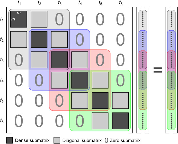
FIGURE 1. Structure of matrix Eq. 1 for solution of the full sequence 4D inversion. Grey, blue, red and green coloured outlines highlight the subproblems solved in sequential windowed 4D inversions, with a window length of three time-steps.

The windowed approach applies the 4D inversion successively to the subproblems highlighted by the coloured outlines, which represent windows of three time-steps length. This simple approach is similar in concept to Schwarz methods, which aim to solve (or precondition) partial differential equations over large domains by decomposing them over smaller, overlapping domains (Kahou et al., 2007; Gander 2008). In Figure 1 the results from the first two time-steps would be produced by solving the grey subproblem, the third time-step by the blue subproblem, the fourth by the red subproblem and the last two time-steps by the green subproblem.

Pre-processing and inversion

For all three sites, the data were pre-processed to remove unreliable data (the following descriptions of each site provide detailed criteria). Where reciprocal pairs of data were measured (LaBrecque et al., 1996), a model based on the reciprocal errors was used to estimate the data errors. At each time-step, the reciprocal errors were binned as a function of the measured transfer resistance, averaged, and a quadratic error model fitted to the mean + two standard deviations of the errors, i.e. an envelope fit designed to encompass ∼95% of the data errors, as introduced by Lesparre et al. (2017). These data error estimates were combined with a simple estimate of the numerical modelling error in the form of a small constant fraction of the measured transfer resistance (Singha et al., 2015). The modelling error estimate was slightly different for each site and was chosen to ensure convergence for all three types of inversion, as one of the codes (E4D) does not have a line search to optimise the step size and can sometimes struggle to converge if the error estimates are too low. Overall this procedure produces a conservative error estimate that reduces the risk of overfitting, albeit at the possible expense of some fine detail in the results. Where the data pre-processing removed measurements, the missing data were interpolated and downweighted in the inversions by assigning a large error to the interpolated value. This error was chosen arbitrarily to be 30 Ω, at least an order-of-magnitude greater than the data error estimates produced by the fitted error models.

Three inversion codes were used to test the methods studied in this paper, since, to the best of our knowledge, no single available code implements all the methods in the same software. The difference inversion of LaBrecque and Yang, 2001 was undertaken using R3t (Binley and Slater, 2020). Note that in the difference inversion, the data errors were propagated according to Wehrer & Slater (2015). The sequential time-lapse inversion was carried out with E4D (Johnson et al., 2010) using the same tetrahedral mesh as for the difference inversion in R3t. E4D implements very flexible combinations of constraints, which we used to impose equally weighted L² spatial smoothness on the changes with respect to the preceding model and also on the current model. For brevity, we refer to this inversion as the time-lapse inversion. Note that E4D could, in principle, also be used to implement the difference inversion but in our tests this was found to be unstable, which we attributed to the lack of a line search on the downhill step at each iteration (R3t by comparison has a very robust line search). The 4D and windowed inversions were performed using Res3DInvX64 from Geotomo Software/Seequent. This works with an internally generated hexahedral grid, so it was not possible to use the same mesh for all inversion types.

Each site had different types of ground truth information available. Borehole records were compared directly to the inverse models to assess whether changes were occurring in expected regions. Where complementary point sensors were used, their data were compared quantitatively to the time-lapse models. In addition, we assessed the internal consistency of the inverse models in order to quantify and compare the discrepancies introduced by the use of short time windows or by the arbitrary choice of the baseline data set. The effects of short time windows were assessed by calculating the differences between these models and those from the full-sequence 4D inversion. This approach is not applicable to the difference and time-lapse inversions since their full sequences are simply assembled from the inversions at each time-step, and so there would be no differences. But unlike the 4D inversions, the results of the difference and time-lapse inversions depend on the choice of the baseline or initial data set, and it is desirable for this choice to have as little influence on the results as possible. Instead, therefore, the discrepancies for these inversions were assessed by calculating the differences between the sequences inverted in the order in which they were acquired (using the first time-step as the baseline) and in reverse order (using the last time-step as the baseline). If this approach were applied to the 4D inversions there should, in principle, be no differences between the forward and reverse order sequences since Eq. 1 is time symmetric. In practice however, numerical errors in its solutions will cause slight differences, so these are also assessed. These measures allowed us to assess the internal consistency of the different types of inversion and assess the effects of their inherent assumptions and limitations. It would be possible to compare the differences between the different types of inversion, although the results would be dependent on the method used to interpolate the models onto common meshes. But any assessment based on this would involve assuming that a particular method was superior. Instead we judged the methods by the degree to which their assumptions and limitations caused internal inconsistencies and by how closely their results correlated with ground truth information and data from complementary sensors.

Results

Site 1—Tracer test in a confined aquifer

An ALERT geoelectrical imaging system was installed at a statutory contaminated land site in Stamford, UK, to monitor changes in groundwater quality in a minor underlying aquifer after the completion of a remediation programme (Wilkinson et al., 2010). The site, a municipal car park built on a former gasworks, was designated as statutory contaminated land due to pollution by a range of polycyclic aromatic hydrocarbons and dissolved phase contaminants. Resistivity monitoring was carried out using multiple vertical electrode arrays installed in purpose-drilled boreholes. As part of the investigation to understand the natural attenuation processes at the site, a saline tracer was injected into the confined aquifer and its motion, dispersion and dilution were visualised directly in the resulting time-lapse ERT imaging sequence.

Two overlapping imaging zones were established on the eastern and southern edges of the site at its south-east corner to image resistivity changes caused by contaminant transport in the direction of the originally assumed groundwater flow. After a year of monitoring these remediation processes, the hydrological regime was better understood and the groundwater flow direction was known to be towards the south-west (approximately in the -x direction, see Figure 2). At this juncture, it was decided to conduct a tracer test that would be imaged in the southern edge zone by the geoelectrical monitoring system. The borehole and site investigation logs showed a 2‒3 m layer of made ground, consisting of bioremediated in-fill material overlying ∼2 m of alluvial clays. Beneath this was a continuous 0.5–1.0 m thick deposit of sands and gravels forming the minor aquifer, underlain by further layers of alluvium, river terrace deposits and Whitby Mudstone bedrock (see Wilkinson et al. (2010) for further details). The aquifer was assumed to be at least semi-confined by the underlying alluvium and bedrock. The strong correlation between the intrusive data and the structure of the initial resistivity image is evident in Figure 2.

FIGURE 2

FIGURE 2. Inverted resistivity, ρ, image of the southern edge of the former gasworks site. Dark grey cylinders show locations of boreholes drilled to install vertical electrode arrays, electrodes are shown by light grey spheres. Blue cylinder shows groundwater monitoring well used to inject saline tracer into the aquifer.

The southern imaging zone comprised ten boreholes, each containing an array of 16 electrodes spaced at 0.5 m intervals (shown as light grey spheres in Figure 2). Four-point transfer resistance measurements were made between all pairs of adjacent boreholes with one current and one potential electrode in each hole. During the previous year-long monitoring period, the current and potential bipoles had a range of vertical extents, but to reduce the measurement time in order to monitor the comparatively fast-moving tracer, only horizontal current and potential bipoles were used (Wilkinson et al., 2010). Measurements were made in reciprocal forward and reverse pairs before the injection of the tracer to assess data quality, but only forward measurements (with the current bipole below the potential bipole) were made during the experiment to minimise the measurement time at each time-step. The differences between the forward and reverse measurements provided reciprocal error estimates, which had a maximum of 2.7%. An envelope error model of the form

$\epsilon =a{R}^2+bR+c,(2)$

where ε is the error and R is the transfer resistance, was fitted to the binned error estimates giving a = 3.05×10^–5 Ω⁻¹, b = 7.91×10^–5, c = 9.14×10^–5 Ω. This model was used to estimate the data errors, which were linearly combined with an assumed modelling error of 3% and used to weight the data in the subsequent inversions. Due to the high quality of the data, no other pre-processing was required and no data were removed before inversion. Note that there was no evidence that the reciprocal error estimates would have changed significantly over time. Contact resistances only changed by ∼10% over the 2 months of the experiment, current levels for all configurations were stable at 150 mA, and the levels and distributions of instrument stacking errors were also very stable.

The instrument made a full set of measurements every 4 h and the tracer test was monitored for a total of 67 days. The tracer, 1.0 m³ (1,000 l) of saline (NaCl) solution at a concentration of 40 g/l, was injected at a rate of ∼4 l/min into a groundwater monitoring well (blue cylinder in Figure 2) that was located adjacent to the imaging zone and screened between depths of 5.0–6.0 m below ground level (bgl). A subset of the resulting data spanning 58 days and comprising 56 time-steps (one per day with days 28 and 29 missing due to data loss) were inverted using 4D inversions (full-sequence and windows of length three and five time-steps, referred to as 3-window and 5-window respectively), independent inversions, time-lapse inversions and difference inversions. All used an L² spatial smoothness constraint and a robust measure of data discrepancy (L¹ norm, or L² with reweighting and/or outlier rejection where L¹ was not available). The 4D inversions applied an L¹ temporal smoothness constraint. A moderate emphasis towards horizontal structure was applied to the 4D, independent and time-lapse inversions (not for the difference inversions as R3t does not offer this option with tetrahedral meshes). The 4D and independent inversions converged to an average absolute data discrepancy of ∼1.6%, and the discrepancies of the time-lapse and difference inversions all reached χ² = 1 (Binley & Slater, 2020). The inverted models are shown as isosurfaces indicating regions where the resistivity has decreased by more than 20% with respect to the initial image. Figure 3 shows these change images from the 4D and independent inversions at selected time-steps, Figure 4 shows those from the time-lapse and difference inversions. Qualitatively all the image sequences look very similar. The motion and dispersal of the tracer were found to be consistent with reasonable estimates of the hydraulic conductivity of the aquifer (Wilkinson et al., 2010). The absence of significant resistivity decreases above 5 m bgl implies that there is little upward migration of the tracer through fissures in the alluvial clay, and that the aquifer is reasonably well confined. There is some evidence of resistivity decrease below 6 m bgl, especially in the first few days near the groundwater monitoring well used for the injection. This is present in all inversions although only visible at the −20% contour level in the 4D and independent inversions. This suggests that either the base or the sides of the injection well were not perfectly sealed, or that the underlying alluvium was not completely impermeable. Some conductive changes also occur in the top 3 m bgl, but these are also mostly smaller than 20% and are probably due to temperature changes rather than infiltration (the surface in the vicinity of the boreholes is covered by black tarmac, which is impermeable and also strongly couples solar radiation into the ground).

FIGURE 3

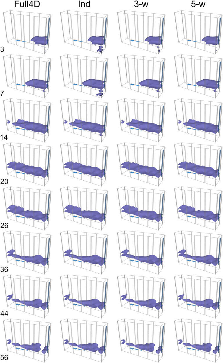
FIGURE 3. Distributions of fractional resistivity change at the former gasworks site for the full sequence 4D, independent, and windowed inversions at the timesteps indicated on the left-hand side. Isosurfaces indicate resistivity changes of −20%. Blue arrows show groundwater flow direction.

FIGURE 4

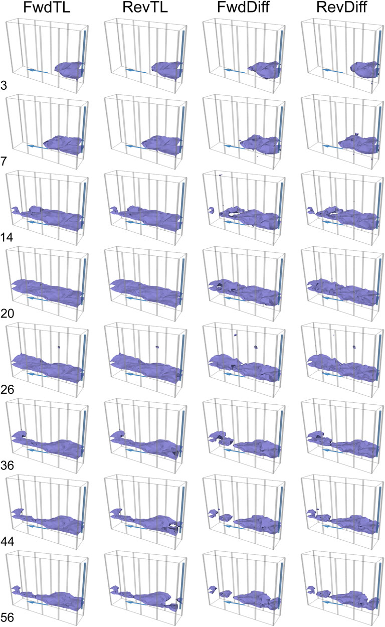
FIGURE 4. Distributions of fractional resistivity change at the former gasworks site for the forward and reverse time-lapse and difference inversions at the timesteps indicated on the left-hand side. Isosurfaces indicate resistivity changes of −20%. Blue arrows show groundwater flow direction.

Figure 5 illustrates the internal consistency of each type of inversion. It shows the median and maximum percentage differences between inverse models, together with the L¹ measure of temporal roughness for the 4D inversions. The differences for the independent (red curves), 3-window 4D (green curves), 5-window 4D (blue curves) and reverse full-sequence 4D (black curves) are all calculated with respect to the forward full-sequence 4D inversion. As expected the independent inversions show the greatest differences, with the discrepancies decreasing progressively with the 3-window and 5-window (note that the difference scale is logarithmic). The differences between the forward and reverse full sequences should theoretically be zero, but in practice are very small (as shown by the black curves) due to the imperfect convergence of the numerical matrix solvers. The consistencies of the difference and time-lapse inversions are assessed from the differences between their forward and reverse sequences. This highlights the effect of the choice of baseline on the resulting inverse models. By this measure, the time-lapse inversion performs similarly to the windowed 4D inversions (slightly better in terms of the median difference, somewhat worse on the maximum difference - dotted curves), whereas the difference inversion performs less well (dashed curves). Note that, as described previously, the method used to assess the independent and windowed inversions would indicate perfect consistency (zero difference within numerical error) if used to test the timelapse and difference inversions, and vice versa. The lowest panel shows the temporal roughness of the independent and 4D inversions. This is noticeably greater for the independent inversions but the windowed 4D inversions are very close to the full-sequence 4D inversion, suggesting that the approximation that the greatest effect of the temporal smoothing comes from the presence of the immediately preceding and succeeding time-steps is valid here.

FIGURE 5

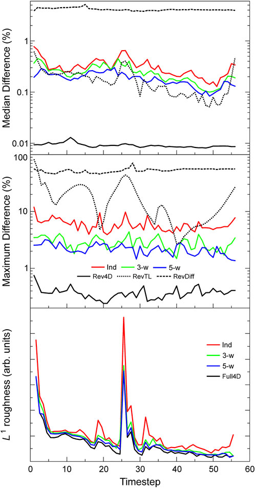
FIGURE 5. Quantitative measures of consistency for each of the inversion methods. Top: median differences between the forward full sequence 4D inversion and the independent, windowed and reverse full sequence 4D inversions, and between the forward and reverse time-lapse inversions, and between the forward and reverse difference inversions. Middle: respective maximum differences. Bottom: L¹ measures of the temporal roughness of the independent, windowed and full sequence 4D inversions.

Site 2—Simulated leakage from a nuclear waste silo

A full-scale field experiment was undertaken to test the ability of cross-borehole ERT to monitor potential leakage from a legacy nuclear waste silo at the Sellafield Site, UK (Kuras et al., 2016). The Magnox Swarf Storage Silos (MSSS) are water-filled concrete silos that received waste from nuclear sites across the UK during their 25-years operational life. In the 1970s, silo liquor is known to have leaked out of the original MSSS building, entering the ground below and creating a plume of contamination (BNFL, 2006). The complex and congested industrial setting of this facility requires the development and use of innovative monitoring technologies to support the safe emptying of the silos. Time-lapse ERT was identified as a promising candidate technology for this application in a desk study prior to the field trials (Kuras et al., 2011).

The trial installation comprised an ALERT system that was connected to six borehole electrode arrays (Kuras et al., 2016), four of which were used in the experiment reported here. These formed an imaging cell of approximately (22 × 7 × 40) m³ (Figure 6), with each borehole containing 40 electrodes at 1 m vertical spacing. The cell was established with two boreholes (BH1 & BH2) adjacent to the MSSS building and the others (BH6 & BH7) 22 m distant. This distance was chosen to represent the full scale of an installation that could span the building (which is 18 m wide). To simulate leaks from the base of the building foundations, conductive tracers were released in shallow boreholes near the centre of the cell (BH4 and BH5) at a depth of 6 m bgl. The hydrogeological context of the site is complex and described in detail in Kuras et al., 2016. In summary, the shallow bedrock is Triassic Sherwood Sandstone, which is encountered at 40–45 m bgl. The superficial geology comprises Quaternary deposits of variable thickness. A layer of made ground typically extends to depths of 1–3 m bgl, although in the direct vicinity of the building the silo foundations reach 6 m bgl. Both the sandstone bedrock and the superficials are of hydrogeological significance and classified as aquifers. At ∼20 m bgl a low-permeability layer of glacial till causes a high degree of hydraulic separation between the upper and lower groundwater systems in the superficial deposits. The lower system is generally in connection with groundwater in the underlying sandstone, and together they are referred to as ‘lower (regional) aquifer’ in Figure 6. The water table is ∼9–10 m bgl and partially saturated conditions prevail in the vadose zone, which is expected to be the primary region of entry for leakage from the building.

FIGURE 6

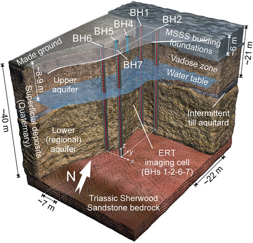
FIGURE 6. Conceptual ground model and geometry of vertical electrode arrays deployed at the MSSS facility. Electrode boreholes are indicated by blue cylinders with red points showing electrodes, shorter blue cylinders indicate tracer release boreholes.

Several tracers were released sequentially to represent different leak scenarios. The tracer considered here had a conductivity of 0.085 S/m at 25 °C, representing a conductivity contrast of 3:1 compared to the groundwater. A volume of 21.8 m³ of the tracer was released over 40 days from BH5. As with Site 1, four-point transfer resistance measurements were made between all pairs of adjacent boreholes with one current and one potential electrode in each hole. Over the course of the experimental programme, full sets of data with a range of dipole vertical extents and separations were collected in reciprocal pairs every second or third day for 2 years. For this tracer, there were 40 time-steps spanning the period from day -1 (the day before the release began) to day 105. The data were filtered prior to inversion to remove problematic measurements. This excluded any data that had been detected to be unreliable by the ALERT system (due to large background potentials, large remnant polarisations, or an inability to pass current), data where the measured waveform was distorted, data involving known problematic electrodes, and data with reciprocal errors of more than 5%. Typically, this filtering only removed ∼9% of the data, and over 99% of the remaining data had reciprocal errors below 1%. A separate envelope error model of the form in Eq. 2 was fitted to the reciprocal error estimates at each time-step. The means and standard deviations of the error model parameters are listed in Table 1. The data error was estimated from these models and was linearly combined with an assumed modelling error of 3% and used to weight the data in the subsequent inversions.

TABLE 1

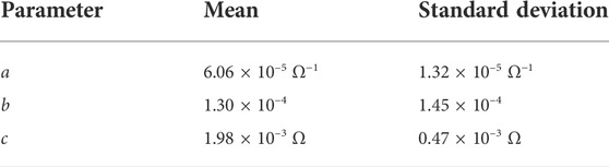
TABLE 1. Means and standard deviations of error model parameters fitted to the Site 2 reciprocal error distributions at each time-step.

The data were inverted using the same constraints as for Site 1, i.e. an L² spatial smoothness constraint and a robust measure of data discrepancy, with an L¹ temporal smoothness constraint for the 4D inversions. A moderate emphasis towards horizontal structure was applied to the 4D, independent and time-lapse inversions. The 4D and independent inversions converged to an average absolute data discrepancy of ∼0.8%, and the discrepancies of the time-lapse and difference inversions all reached χ² = 1. Images of resistivity changes were plotted relative to the first time-step (day -1) and show different spatial patterns and temporal evolution of change in distinct regions of the model. Figure 7 shows an example, with regions where the ground had become more conductive/resistive shown in blue/red respectively and filled isosurfaces showing changes in resistivity below -2%. In the vadose zone, a general decrease in resistivity over time was observed, which was attributed to the injection of the liquor simulant tracer at BH5 (location indicated by the blue arrow) and the rising temperatures during the monitoring period. This was punctuated by isolated changes relating to run-off of snow melt and de-icing salt and infiltration from rainfall. In the upper saturated zone, the conductive changes associated with the ingress of the tracer are localised in a sub horizontal band highlighted by the black contour between regions of conductive and resistive changes in Figure 7. This band coincides with zones of historic contamination (shown by green cylinders) that were detected in sediment cores retrieved from the boreholes. This led to the conclusion that the simulant tracer had reoccupied a preferred contaminant flow pathway that appeared to have been active in the past (Kuras et al., 2016).

FIGURE 7

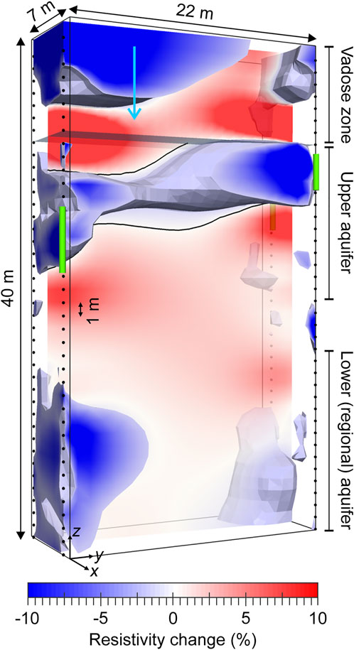
FIGURE 7. Annotated example distribution of fractional resistivity change in the imaging region bounded by the vertical borehole electrode arrays at MSSS. Blue arrow indicates tracer injection location, green cylinders show regions of historic contamination detected in borehole sediment cores (data ^© Sellafield Ltd.). Isosurfaces bound regions of resistive change below −2%. Black line is the 0% change contour, assumed to delineate the preferential pathway reoccupied by the tracer.

The evolution of these changes is shown for selected time-steps for the 4D and independent inversions in Figure 8 and for the time-lapse and difference inversions in Figure 9. As with Site 1, the image sequences look qualitatively similar, although there are more visible differences between the independent and 4D inversions and between the forward and reverse sequence difference and time-lapse inversions. The appearance of a continuous sub horizontal band of conductive change associated with the preferential pathway is apparent in most of the inversions by, or at some time after, time-step 16 (day 33) with the exception of the forward sequence difference inversion, in which it never becomes laterally continuous. The contrast of the pathway feature is greatest in the regions near the boreholes, where the sensitivity and model resolution are highest. In these regions, the contrast continues to increase after the tracer injection finishes on day 40 (after time-step 19). This was attributed to remnant tracer previously held up in the vadose zone being flushed into the pathway by following rainfall thereby extending the effects of the injection well beyond the time that the pumps were switched off. Consistent with this interpretation, the contrast of the changes in all parts of the pathway (whether near the boreholes or towards the centre of the model) were found to increase with time in the 4D inversions. However, the time-lapse and difference inversions are less consistent, exhibiting inconsistent temporal patterns of increasing and decreasing contrast in the pathway region.

FIGURE 8

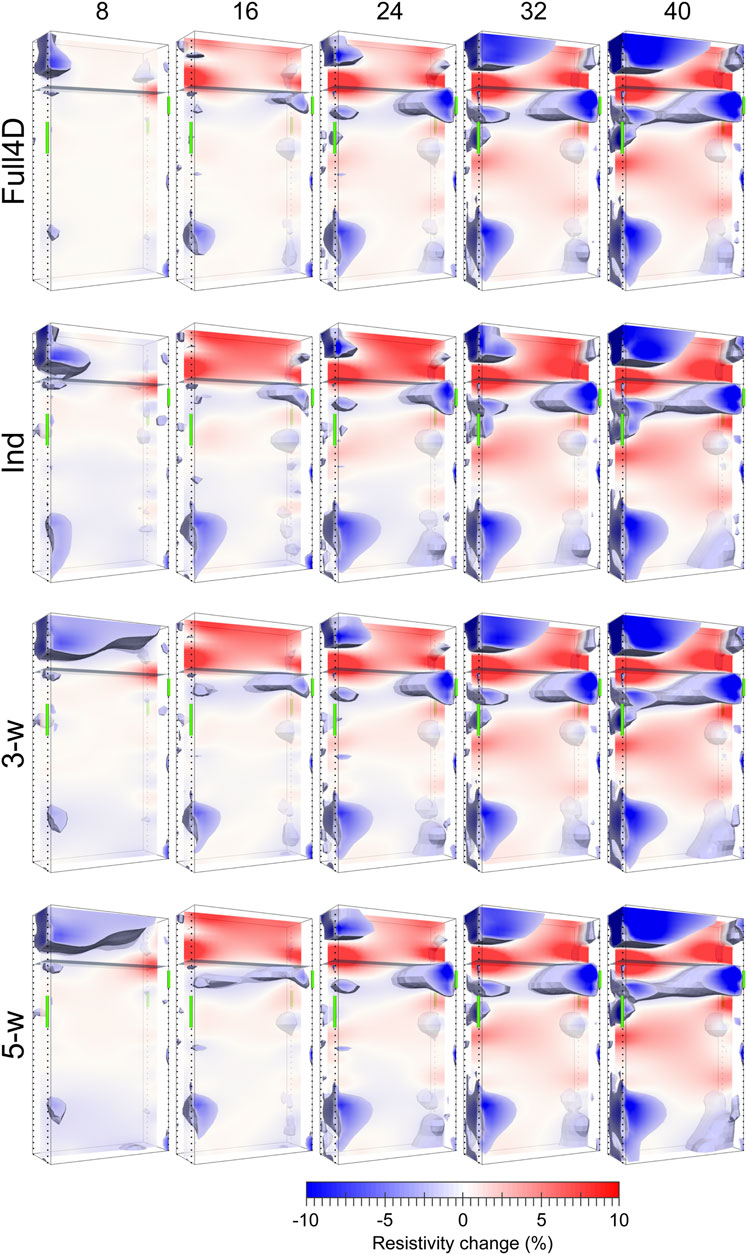
FIGURE 8. Distributions of fractional resistivity change at MSSS for the full sequence 4D, independent, and windowed inversions at the timesteps indicated at the top of the diagram. Isosurfaces indicate resistivity changes of < −2%. Green cylinders show regions of historic contamination (data ^© Sellafield Ltd.).

FIGURE 9

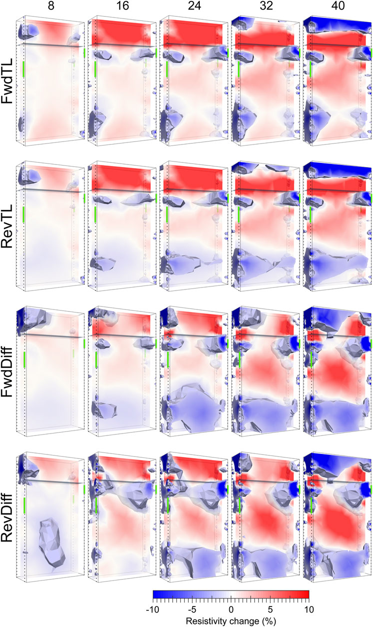
FIGURE 9. Distributions of fractional resistivity change at MSSS for the forward and reverse time-lapse and difference inversions at the timesteps indicated at the top of the diagram. Isosurfaces indicate resistivity changes of < −2%. Green cylinders show regions of historic contamination (data ^© Sellafield Ltd.).

Figure 10 shows the median and maximum percentage differences between the different types of inversion, and the L¹ measure of temporal roughness for the 4D inversions. As with Site 1, the inconsistencies between the windowed/independent inversions and the full sequence 4D inversion are greatest for the independent inversions and decrease progressively with the length of the window. The inconsistencies between the forward and reverse full sequence 4D inversions are again very small. The discrepancies between the forward and reverse time-lapse inversions are slightly lower than those for the windowed 4D inversions, whereas those for the difference inversion are somewhat greater. The lowest panel shows the temporal roughness of the 4D inversions, which is greatest for the independent inversions and decreases with the window length of the 4D inversions, although the assumption that the greatest effect of the temporal smoothing comes from the presence of the immediately preceding and succeeding time-steps appears to hold less strongly here than it did for Site 1.

FIGURE 10

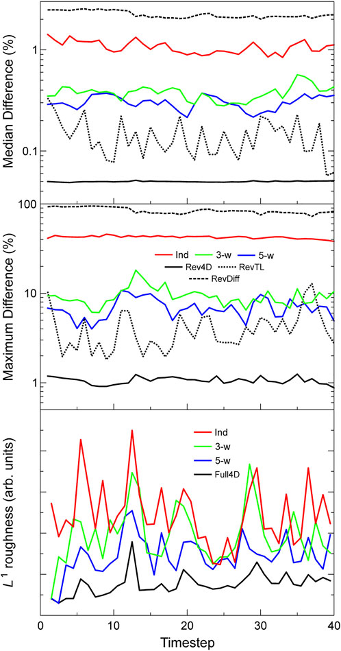
FIGURE 10. Quantitative measures of consistency for each of the inversion methods. Top: median differences between the forward full sequence 4D inversion and the independent, windowed and reverse full sequence 4D inversions, and between the forward and reverse time-lapse inversions, and between the forward and reverse difference inversions. Middle: respective maximum differences. Bottom: L¹ measures of the temporal roughness of the independent, windowed and full sequence 4D inversions.

Site 3—Simulated leakage from a buried water utility pipe

An experimental site was established to test the ability of geophysical techniques to monitor the long-term condition of ground subject to leakage from failed water utility pipes. The methods studied were ERT (Inauen et al., 2016), Time-Domain Reflectometry (TDR) (Curioni et al., 2019) and Multi-channel Analysis of Surface Waves (MASW) (Dashwood et al., 2020). The site was located in Blagdon, UK, and consisted of an area of grass-covered field approximately (10 × 10) m² surrounded by large conifer trees. The site geology comprises the Sidmouth Mudstone Formation of the Mercia Mudstone Group, which is characterised by red-brown mudstone and siltstone. Material excavated from trenches was interpreted as red-brown clayey silt with gravel-to cobble-sized inclusions of dolomitic siltstone and unweathered mudstone (Dashwood et al., 2020). The water table was estimated to be at approximately 2.2 m bgl.

Two trenches were dug on the site, both 8 m long and 1.2 m wide and deep. An 8 m long section of standard 25 mm external diameter plastic water pipe was installed in each trench at 0.7 m bgl and connected to the water mains network. Each pipe had a stop cock to control the water flow and a 3 mm diameter hole approximately half way along its length from which water could leak. The trenches were back-filled with the excavated soil and compacted until approximately level with the surrounding ground. One of the trenches was monitored using ERT, MASW and a small number of TDR sensors, the other with a dense array of TDR sensors. The second trench was to the south-east of the first. A schematic plan view of the installation is shown in Figure 11A. A grid array of 13 × 13 ERT electrodes was installed at the surface with spacings of 0.5 m in the x and y directions. TDR sensors were buried coincident with the (x, y) leak location at depths of 0.10, 0.35, 0.60, 0.80, 1.00 and 1.20 m bgl. A PRIME geoelectrical imaging system was connected to the electrodes and used to make all possible inline dipole-dipole measurements along the x, y and intercardinal diagonal directions. Full sets of measurements were made every 4 hours in reciprocal pairs. The data quality was very good, with 95% of the data having reciprocal errors below 1%, and 99% of the data below 5%. A separate envelope error model, of the form in Eq. 2, was fitted to the reciprocal error estimates at each time-step. The means and standard deviations of the error model parameters are listed in Table 2. The data error was estimated from these models and was linearly combined with an assumed modelling error of 2.5% and used to weight the data in the subsequent inversions.

FIGURE 11

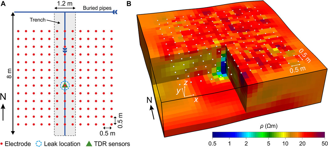
FIGURE 11. (A) Array of 13 × 13 electrodes (red dots) used to monitor the simulated leak from utility pipe buried at 0.7 m depth. Light grey region indicates location of trench, blue dotted lines show leak location, and green triangle indicates position of vertical array of TDR sensors. (B) Inverted resistivity, ρ, image of the ERT and TDR monitoring trench at Site 3 showing electrode locations (white dots). A strong conductive anomaly is present coincident with the locations of the TDR probes.

TABLE 2

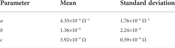
TABLE 2. Means and standard deviations of error model parameters fitted to the Site 3 reciprocal error distributions at each time-step.

ERT monitoring was carried out for 30 days, with data collection starting 2 days before the leaking pipe was opened. The leak was open for 29.75 h at a nominal rate of 1.5 l/min, resulting in a measured total leak volume of 2.10 m³ of water. The inverted sequences of data presented here comprise 49 time-steps with variable periods, ranging from 4 h, during and immediately after the leak, to 16 h (with two longer isolated gaps of 48 and 88 h due to data loss). The resistivity data were inverted using L² spatial smoothness constraints and a robust measure of data discrepancy, with an L² temporal smoothness constraint for the 4D inversions. The 4D and independent inversions converged to an average absolute data discrepancy of ∼2.1%, and the discrepancies of the time-lapse and difference inversions all reached χ² = 1. A baseline resistivity image is shown in Figure 11B. Of particular note is a strongly conductive anomaly directly beneath the injection point. This was attributed to the presence and electrical connections of the metallic TDR sensors.

The evolution of the inverted resistivity models is shown in terms of resistivity change at selected time-steps in Figure 12 for the 4D and independent inversions and Figure 13 for the time-lapse and difference inversions. The model cells are shown where the resistivity change with respect to the first time-step is < -7.5%. Three distinct periods of change are visible. The leak is switched on between time-steps 4 and 5, and off between 11 and 12. At time-step 5, a region of conductive change appears below and centred on the leak location, spreading out radially. The models at time-step 13 show this region having spread from the injection point. By time-step 19, a new region of conductive change has started to form in the south-eastern corner of the models. This moves further towards the centre of the model and/or becomes stronger until about time-step 34. This feature is associated with a larger, faster leak (5.20 m³ over 25.75 h) that was switched on in the second (TDR) trench to the south-east immediately after the leak was switched off in the ERT trench. This more conductive feature begins to dissipate around time-step 36, coinciding with the onset of intense rainfall between timesteps 36 and 39, and again between timesteps 48 and 49. The effect of infiltration from the rainfall is to decrease the resistivity in the top ∼1 m of the model across most of the imaging area, with the exception of the south-eastern corner. This part of the site was sheltered under the canopy of one of the large conifer trees.

FIGURE 12

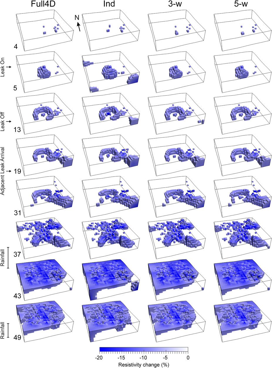
FIGURE 12. Distributions of fractional resistivity change at Site 3 for the full sequence 4D, independent, and windowed inversions at the timesteps indicated on the left-hand side. Only model cells with resistivity changes below −20% are shown.

FIGURE 13

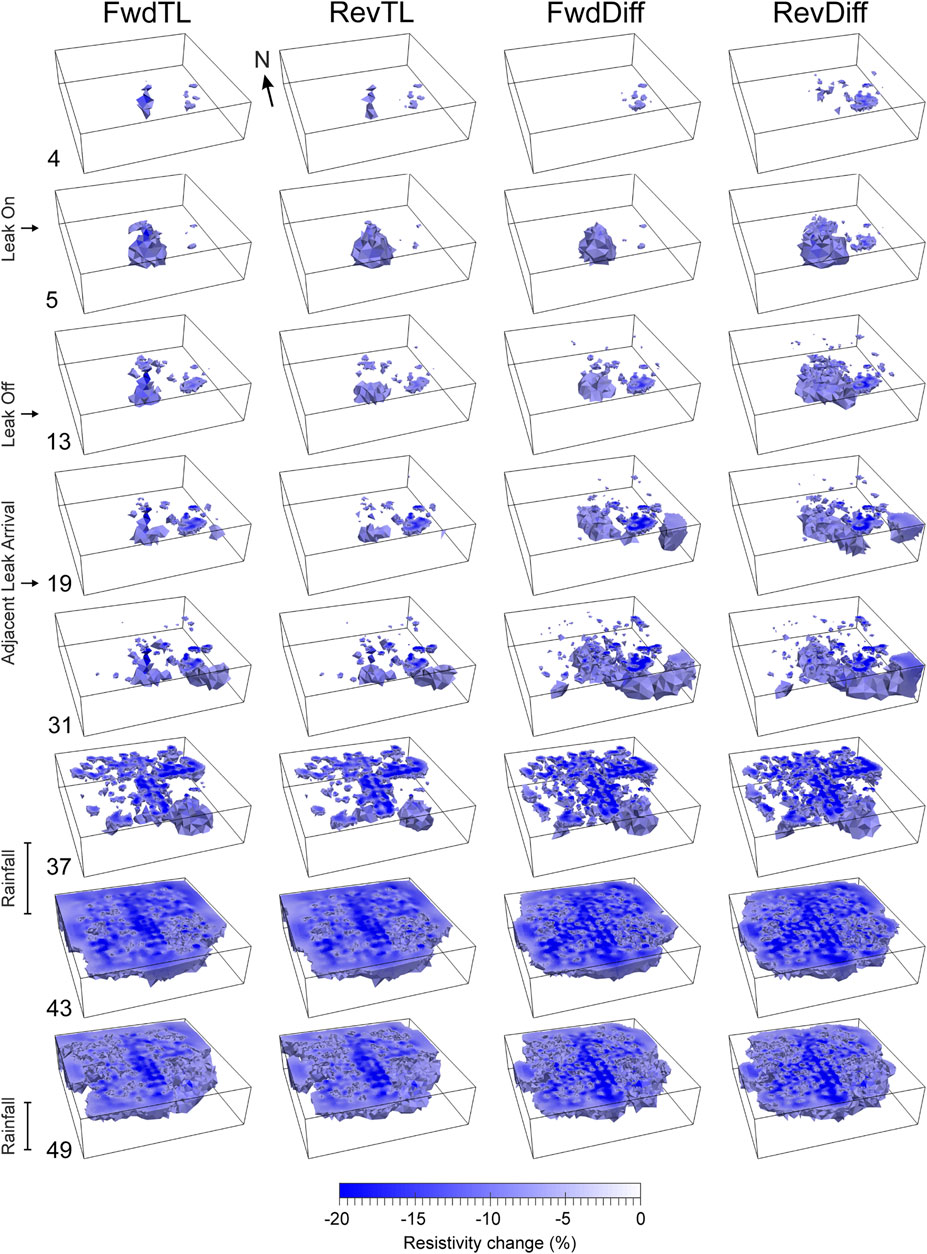
FIGURE 13. Distributions of fractional resistivity change at Site 3 for the forward and reverse time-lapse and difference inversions at the timesteps indicated on the left-hand side. Only model cells with resistivity changes below -20% are shown.

As with the other sites in this paper, the different types of inversion produced qualitatively similar spatial and temporal patterns of change, although the differences between them were more pronounced. The most notable of these were that the effects of the water from the leak seemed to spread out to the greatest lateral extents in the 4D inversions, followed by the difference inversions, with the time-lapse inversions showing the least lateral spread. It is unclear which of these situations most closely resembled the actual site conditions. But another notable set of temporal changes, the ingress of water from the leak experiment in the second trench, seems to be most realistically reconstructed by the 4D inversions, in that the conductive changes move in towards the centre of the model from the edge, rather than an isolated conductive region appearing, strengthening and decaying while exhibiting little to no movement, as observed in the time-lapse inversions. The difference inversions exhibited intermediate behaviour with some similarities to both, a more isolated region appearing near the corner and then extending towards the centre.

At this site, it was also possible to assess the quality of the ERT reconstructions quantitatively. The TDR sensors measured the bulk electrical conductivity, which can be compared with conductivities derived from the resistivity models at the same points. But the presence of the strong conductive anomaly coincident with the TDR probes (Figure 11B) complicates this comparison in two ways: the ERT conductivities will be much greater than the directly measured values; and the relationship between the ERT and TDR conductivities will be non-linear (although still monotonic). To counteract the greater conductivities from the ERT models, we compare the relative changes in the TDR and ERT conductivities (rather than the absolute changes or values). To assess the degree of association between the changes over time, we compare the TDR and ERT relative conductivity changes using the Kendall rank correlation coefficient, τ, which is a robust measure of correlation that assesses the strength and direction of any general monotonic relationship between two variables. Figure 14B shows the relative changes in conductivity over time as measured by the TDR probes. Increases in conductivity due to the effects of the active leak (during the period indicated by the light blue vertical bar) and infiltration (during the periods of positive estimated effective rainfall, shown in Figure 14A) are clearly visible. Similar plots are shown in Figure 14C–Figure 14J for conductivities extracted (by distance weighted average of neighbouring cells) at the same locations from the resistivity models for each of the different inversion types (note that the results from the forward and reverse full-sequence 4D inversions in Figure 14F are indistinguishable at this scale). All the inversions exhibit conductivity changes due to the leak and infiltration that are qualitatively similar to those observed in the TDR data. The correlation coefficient, τ, was calculated for each TDR sensor position and its average value for each inversion type is shown in the respective panel. All indicate strong positive correlations with the directly measured data. The strongest are produced by the 4D inversions, followed by the difference inversions, with the time-lapse inversions exhibiting the weakest correlations.

FIGURE 14

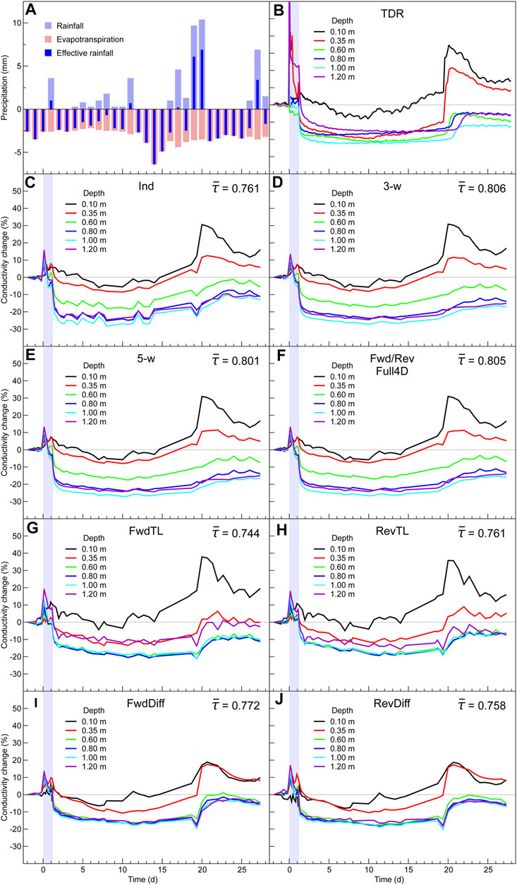
FIGURE 14. (A) Rainfall, estimated evapotranspiration and effective rainfall during the leak experiment (B) Relative changes in conductivity measured by the TDR probes (data ^© University of Birmingham) (C–J) relative changes in conductivity extracted from the independent, 3-window 4D, 5-window 4D, forward/reverse full sequence 4D, forward time-lapse, reverse time-lapse, forward difference and reverse difference inversions respectively. $\overline{\tau }$ is the average Kendall rank correlation coefficient between the TDR and inverse model conductivity changes across all TDR sensor locations.

Figure 15 shows the median and maximum percentage differences between different types of inversion, and the L² measure of temporal roughness for the 4D inversions. As with Sites 1 and 2, the inconsistencies between the windowed/independent inversions and the full sequence 4D inversion are greatest for the independent inversions and decrease progressively with the length of the window. The inconsistencies between the forward and reverse full sequence 4D inversions are again very small. The discrepancies between the forward and reverse time-lapse inversions are slightly greater than those for the windowed 4D inversions, and those for the difference inversion are somewhat greater again. The lowest panel shows the temporal roughness of the 4D inversions, which is greatest for the independent inversions and decreases rapidly with the window length of the 4D inversions (to the extent that the 5-window and full sequence results cannot be distinguished in Figure 15). This is similar to the findings at Site 1 and suggests again that the greatest effect of the temporal smoothing is arising from the immediately preceding and succeeding time-steps.

FIGURE 15

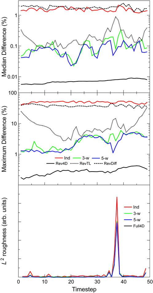
FIGURE 15. Quantitative measures of consistency for each of the inversion methods. Top: median differences between the forward full sequence 4D inversion and the independent, windowed and reverse full sequence 4D inversions, and between the forward and reverse time-lapse inversions, and between the forward and reverse difference inversions. Middle: respective maximum differences. Bottom: L² measures of the temporal roughness of the independent, windowed and full sequence 4D inversions (note that here the 5-w results overplot the Full4D).

Discussion

To assess the overall performance of the different methods, we consider measures of their consistency, qualitative assessments of the behaviour of the changes in their model sequences, and quantitative comparisons with other sensor data where available.

Table 3 provides an overall assessment of the consistency of the inversions for each site in terms of the average over all time-steps of the median and maximum percentage differences (which are shown in Figure 5, Figure 10 & Figure 15). For the independent and windowed inversions, these are assessed by comparison with the full-sequence 4D inversion, the time-lapse and difference inversions are assessed by comparison of the forward and reverse time-sequences. The greatest consistencies (smallest differences) occur using the windowed 4D inversions in three cases (Site 1 maximum difference and Site 3 median and maximum differences) and using the time-lapse inversions in the other three (Site 1 median differences and Site 2 median and maximum differences). For comparison, the differences are also shown for the reverse sequence 4D inversions. These should be zero and hence are indicative of the level of error in the numerical solutions of Eq. 1.

TABLE 3

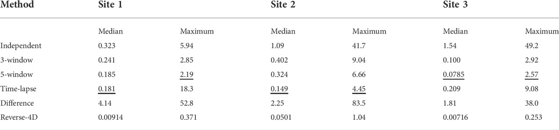
TABLE 3. Consistency measures of the tested inversion methods in terms of averaged percentage median and maximum differences. The method giving greatest consitency (smallest difference) is underlined for each measure and site.

For the independent and windowed inversions, we also assess the temporal roughness of the inverse model sequences. Table 4 gives the total sequence roughness (from the data shown in Figure 5, Figure 10 & Figure 15) in arbitrary units relative to the roughness of the full 4D sequence.

TABLE 4

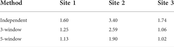
TABLE 4. Total temporal roughness of independent and windowed inversions relative to full sequence 4D inversion.

In all cases, in terms of both median and maximum difference and temporal roughness, the greatest improvements with increasing window length occur between the independent and 3-window inversions rather than between the 3- and 5-window inversions. This suggests that using a short window of three time-steps would be sufficient to gain most of the benefits of 4D inversion, while still being able to deliver results in near real-time from an automated geoelectrical monitoring system. It is worth noting that, as implemented in Res3DInvX64, the processing time taken for the 4D inversion scales linearly with the number of time steps. So, although there is a time penalty for using windowed rather than independent inversion, it is not severe.

For Site 1, the qualitative behaviours of the changes from all types of inversion are very similar and cannot be distinguished in terms of the known ground and hydrological conditions. At Site 2, the spatial distributions of change are also similar between the inversion types, although there are some differences in their temporal evolution. In the upper aquifer, the tracer appears to occupy a preferential pathway identified in the borehole logs by the presence of radioactive contamination caused by a previous leak from the silo. In the 4D inversions (windowed or full-sequence), the magnitude of the conductive change in the pathway continues to increase over time, assumed to be caused initially by the release of the tracer and then by remnant tracer being flushed through by subsequent rainfall (Kuras et al., 2016). In the time-lapse and difference inversions, the temporal evolution of the conductivity contrast in this pathway is inconsistent, showing regions of increase and decrease even while the tracer release was continuing. For Site 3, differences were observed in terms of the lateral extent to which the leaking water spread, and the reconstruction of water ingress from the other leak experiment at the site. Although no argument can be made regarding the most accurate reconstruction of the former, the latter seemed to be most reasonably reconstructed in the 4D inversions (in terms of a continuously evolving conductive anomaly moving inwards from the direction of the second experiment). It should be noted that only applying arbitrary resistivity thresholds to display plume behaviour can overemphasise small differences between time series, but we observed that the overall qualitative behaviour of the different inversion types appeared similar at a weaker threshold (-5%). More importantly at Site 3, quantitative comparisons with direct measurements of electrical conductivity showed that the TDR data were most strongly correlated with the 4D inversions (windowed or full-sequence) rather than the difference or time-lapse inversions.

In comparison with the independent inversions, we note that, although windowed inversions 1) improve the reconstruction of qualitatively expected behaviour, 2) strengthen quantitative comparisons with directly measured data, and 3) improve the consistency and temporal smoothness, the degree of improvement with window length differs from one site to another. It is to be expected that when subsurface changes are weaker, noise levels are higher, or larger regions of the model are far from the electrodes and therefore poorly resolved by the data, the relative importance of the temporal regularisation will be more pronounced and the degree to which the temporal smoothing is most strongly affected by the immediately neighbouring time-steps will be reduced. At Site 2 for example, the tracer contrast is relatively weak and the spacing of the boreholes in the y-direction is relatively large, leaving the changes in the central regions of the model comparatively poorly resolved. This could account for the slower improvement in consistency and temporal smoothness with window length than observed at the other sites. We have also noted similar effects in models where the number of parameter cells exceeds the number of data, such as from irregular and/or curved linear electrode arrays in complex topography with significant off-line resistivity variations. In these cases, 3D models are necessary with finely discretised surfaces to capture the topographic variations, causing the inverse problem to be underdetermined to a greater degree than usual and more reliant on the constraints.

Another factor that could affect the length of the window required to approximate the full-sequence inversion adequately is how rapidly the induced resistivity variation occurs and the rate at which data are acquired. Most time-lapse inversion methods assume that data are effectively acquired simultaneously (with an exception being the 4D implementation of Kim et al. (2009)). Therefore measurement sequences are typically rapid compared to the expected timescales of the induced variations to avoid temporal blurring (Wilkinson et al., 2010). Nevertheless, the periods between sets of measurements could still be long (e.g., to avoid excessive power usage in remote monitoring installations) and therefore significant resistivity changes could occur between adjacent time-steps in the inversion. In these cases, using an L¹ rather than L² temporal constraint should allow a shorter window to better approximate the full-sequence inversion as it applies a comparatively lower penalty to large temporal changes.

While the magnitude and rate of the temporal changes can affect the accuracy of the windowed approximation, we believe that, in general, the spatial complexity of the resistivity structure and the changes within it should not. Whether conducting a one-off survey or time-lapse monitoring, the experimental design (electrode spacing and measurements) should provide sufficient model resolution to resolve structures of interest (e.g. thin layers) and the spatial constraints in the inversion should be suitably implemented to reveal complex structure (e.g. correctly oriented anisotropic smoothing for strata with pronounced dips and/or reduction of smoothing across known boundaries). There could conceivably be cases in which the spatial structure of the resistivity changes is different to that of the underlying resistivity distribution, and here different spatial priors would be needed for the distribution and the changes. This would require a modification of Eq. 1 but should not affect the validity of the windowed inversion approximation.

Conclusion

Overall, the observations from our inversions of real field data support conclusions from previous synthetic modelling studies (Kim et al., 2009, 2013; Loke et al., 2014) that 4D inversions produce more accurate reconstructions of temporal changes than other methods. We tested both L¹ and L² temporal smoothness constraints and observed that, in particular, L¹ constraints seem particularly well-suited to resolving localised changes, such as the preferential pathway at Site 2. This supports the previous observations of Kim et al. (2013).

Our results indicate that short time-window 4D inversions are a suitable method to approximate the results of full sequence 4D inversions in a near real-time automated processing context. Most of the advantages over independent inversion, in terms of consistency and temporal smoothness, are obtained using a window of only three time-steps length. In particular, at Site 3 where directly measured intrusive data were available for comparison, we note that the correlations with the windowed inversion results were very close to the full-sequence inversions, and stronger than the other methods tested. We note that the windowed inversions also seem to preserve the recovery of qualitatively realistic behaviour of subsurface moisture content changes exhibited by the 4D full-sequence inversions.

The necessary reliance on different inversion software for the different inverse methods means that there is an element of testing the implementation of the method (e.g. presence or absence of a downhill line search) and discretisation of the model (e.g., tetrahedral or hexahedral cells) as well as the method itself. Nevertheless, our results clearly show that the windowed 4D inversions perform similarly to the full-sequence 4D inversions, and better than the independent inversions. They strongly suggest that windowed 4D inversions are comparable with the sequential time-lapse inversions in terms of consistency of results, and perform better in terms of the quantitative and qualitative assessments model accuracy. They also appear to out-perform difference inversions in both aspects. In addition, the 4D inversions have the advantage of being independent of a baseline reference which, especially for the difference inversion, can have a significant effect on the resulting model.

In the context of automated inversion of time-lapse ERT monitoring data, if the window has length n_w then the results for the time-step of interest, t, at the centre of the window, would be delivered after a delay of (n_w−1)/2 time-steps. This delay could be seen as a disadvantage of the windowed 4D inversion approach. But provisional results would be available immediately from the window containing time-step t at its leading edge, rather than its centre. For clarity, in this paper we have restricted the scope to assessing the quality of the inversions from the window centres, but our experience is that the provisional inversions from the leading edges of these preceding windows are of similar, albeit slightly lower, quality (Wilkinson et al., 2019), and we are studying the degree of difference exhibited by these provisional results in detail for future publication.

Data availability statement

The raw data supporting the conclusion of this article will be made available by the authors, without undue reservation.

Author contributions

PW–Data processing, inversion, technique comparison, Site 1 experiment and project management, manuscript preparation JC–Site 3 experiment and project management, monitoring concept development lead, results interpretation all sites PM–Monitoring hardware lead for all sites, Sites 1 and 2 experimental design and installation OK–Site 2 experiment design, project management and results interpretation CI–Site 3 ERT experiment site works and operation, results interpretation RS–Site 3 ERT experiment installation and operation GC–Site 3 TDR installation, operation, results and interpretation SU–Site 2 experiment operation JG–Site 2 hydrogeological and ground truth input and interpretation, ERT experiment design NA–Site 2 operator, site management, problem specification and ownership, ERT experiment design.

Funding

The authors declare that this study received funding from Sellafield Ltd. The funder had the following involvement with the study: Site operation and management, problem specification and ownership, ERT experiment design.

Acknowledgments

We are very grateful to South Kesteven District Council, Sellafield Ltd. and National Nuclear Laboratory, and Bristol Water PLC for their generous permissions, assistance and collaboration with the field experiments carried out at Sites 1, 2, and 3 respectively. This work was supported by the British Geological Survey via NERC national capability. The work at Site 1 was supported by a grant from the Technology Strategy Board (www.innovateuk.org; project TP/5/CON/6/I/H0048B). The work at Site 2 was supported by funding from Sellafield Ltd. The work at Site 3 was supported by a United Kingdom Engineering and Physical Sciences Research Council grant (EP/KP021699/1). Wilkinson, Chambers, Meldrum, Kuras, Inauen, Swift and Uhlemann publish with the permission of the Executive Director, British Geological Survey (UKRI-NERC). We extend our thanks to the two reviewers whose comments helped to improve the manuscript. For the purpose of open access, the author has applied a Creative Commons Attribution (CC BY) licence [where permitted by UKRI, “Open Government Licence” or “Creative Commons Attribution No-derivatives (CC BY-ND) licence”] to any Author Accepted Manuscript version arising.

Conflict of interest

NA was employed by Sellafield Ltd

The remaining authors declare that the research was conducted in the absence of any commercial or financial relationships that could be construed as a potential conflict of interest.

Publisher’s note

All claims expressed in this article are solely those of the authors and do not necessarily represent those of their affiliated organizations, or those of the publisher, the editors and the reviewers. Any product that may be evaluated in this article, or claim that may be made by its manufacturer, is not guaranteed or endorsed by the publisher.

References

Arosio, D., Munda, S., Tresoldi, G., Papini, M., Longoni, L., and Zanzi, L. (2017). A customized resistivity system for monitoring saturation and seepage in earthen levees: Installation and validation. Open Geosci. 9, 457–467. doi:10.1515/geo-2017-0035

CrossRef Full Text | Google Scholar

Binley, A., Hubbard, S. S., Huisman, J. A., Revil, A., Robinson, D. A., Singha, K., et al. (2015). The emergence of hydrogeophysics for improved understanding of subsurface processes over multiple scales. Water Resour. Res. 51, 3837–3866. doi:10.1002/2015wr017016

PubMed Abstract | CrossRef Full Text | Google Scholar

Binley, A., and Slater, L. (2020). Resistivity and induced polarization: Theory and applications to the near-surface Earth. Cambridge, UK: Cambridge University Press.

Google Scholar

BNFL (2006). Decommissioning B38. New civil engineer. London, UK: EMAP.

Google Scholar

Boyd, J., Chambers, J. E., Wilkinson, P. B., Watlet, A., Kirkham, M., Jones, L., et al. (2021). A linked geomorphological and geophysical modelling methodology applied to an active landslide. Landslides 18, 2689–2704. doi:10.1007/s10346-021-01666-w

CrossRef Full Text | Google Scholar

Chambers, J. E., Meldrum, P. I., Wilkinson, P. B., Gunn, D. A., Watlet, A., Dashwood, B., et al. (2021). “Geophysical remote condition monitoring of transportation infrastructure slopes,” in Proceedings near surface geoscience 2021 (Bordeaux, France.

CrossRef Full Text | Google Scholar

Curioni, G., Chapman, D. N., Royal, A. C. D., Metje, N., Dashwood, B., Gunn, D. A., et al. (2019). Time domain reflectometry (TDR) potential for soil condition monitoring of geotechnical assets. Can. Geotech. J. 56, 942–955. doi:10.1139/cgj-2017-0618

CrossRef Full Text | Google Scholar

Dashwood, B., Gunn, D. A., Curioni, G., Inauen, C. M., Swift, R. T., Chapman, D. N., et al. (2020). Surface wave surveys for imaging ground property changes due to a leaking water pipe. J. Appl. Geophys. 174, 103923. doi:10.1016/j.jappgeo.2019.103923

CrossRef Full Text | Google Scholar

Gander, M. J. (2008). Schwarz methods over the course of time. Electron. Trans. Numer. Analysis 31, 228–255.

Google Scholar

Holmes, J., Chambers, J. E., Meldrum, P. I., Wilkinson, P. B., Boyd, J., Williamson, P., et al. (2020). Four-dimensional electrical resistivity tomography for continuous, near-real-time monitoring of a landslide affecting transport infrastructure in British Columbia, Canada. Near Surf. Geophys. 18, 337–351. doi:10.1002/nsg.12102

CrossRef Full Text | Google Scholar

Inauen, C. M., Chambers, J. E., Wilkinson, P. B., Meldrum, P. I., Swift, R. T., Uhlemann, S., et al. (2016). “4D ERT monitoring of subsurface water pipe leakage during a controlled field experiment,” in Proceedings AGU fall meeting 2016 (San Francicso, CA, USA: American Geophysical Union).

Google Scholar

Johnson, T. C., Versteeg, R. J., Ward, A., Day-Lewis, F. D., and Revil, A. (2010). Improved hydrogeophysical characterization and monitoring through parallel modeling and inversion of time-domain resistivity and induced polarization data. Geophysics 75, Wa27–Wa41. doi:10.1190/1.3475513

CrossRef Full Text | Google Scholar

Kahou, G. A. A., Kamgnia, E., and Philippe, B. (2007). An explicit formulation of the multiplicative Schwarz preconditioner. Appl. Numer. Math. 57, 1197–1213. doi:10.1016/j.apnum.2007.01.009

CrossRef Full Text | Google Scholar

Karaoulis, M. C., Kim, J. H., and Tsourlos, P. I. (2011). 4D active time constrained resistivity inversion. J. Appl. Geophys. 73, 25–34. doi:10.1016/j.jappgeo.2010.11.002

CrossRef Full Text | Google Scholar

Karaoulis, M. C., Tsourlos, P. I., Kim, J. H., and Revil, A. (2014). 4D time-lapse ERT inversion: Introducing combined time and space constraints. Near Surf. Geophys. 12, 25–34. doi:10.3997/1873-0604.2013004

CrossRef Full Text | Google Scholar

Kim, J. H., Supper, R., Tsourlos, P., and Yi, M. J. (2013). Four-dimensional inversion of resistivity monitoring data through Lp norm minimizations. Geophys. J. Int. 195, 1640–1656. doi:10.1093/gji/ggt324

CrossRef Full Text | Google Scholar

Kim, J. H., Yi, M. J., Park, S. G., and Kim, J. G. (2009). 4-D inversion of DC resistivity monitoring data acquired over a dynamically changing Earth model. J. Appl. Geophys. 68, 522–532. doi:10.1016/j.jappgeo.2009.03.002

CrossRef Full Text | Google Scholar

Kuras, O., Pritchard, J. D., Meldrum, P. I., Chambers, J. E., Wilkinson, P. B., Ogilvy, R. D., et al. (2009). Monitoring hydraulic processes with automated time-lapse electrical resistivity tomography (ALERT). Comptes Rendus Geosci. 341, 868–885. doi:10.1016/j.crte.2009.07.010

CrossRef Full Text | Google Scholar

Kuras, O., Wilkinson, P. B., Meldrum, P. I., Oxby, L. S., Uhlemann, S., Chambers, J. E., et al. (2016). Geoelectrical monitoring of simulated subsurface leakage to support high-hazard nuclear decommissioning at the Sellafield Site, UK. Sci. Total Environ. 566-567, 350–359. doi:10.1016/j.scitotenv.2016.04.212

PubMed Abstract | CrossRef Full Text | Google Scholar

Kuras, O., Wilkinson, P. B., White, J. C., Chambers, J. E., Meldrum, P. I., and Ogilvy, R. D. (2011). MSSS leak mitigation - leak detection phase 3: Desk study for ERT technology. Commissioned report CR/11/053. Nottingham: British Geological Survey.

Google Scholar

LaBrecque, D. J., Miletto, M., Daily, W., Ramirez, A., and Owen, E. (1996). The effects of noise on Occam’s inversion of resistivity tomography data. Geophysics 61, 538–548. doi:10.1190/1.1443980

CrossRef Full Text | Google Scholar

LaBrecque, D. J., and Yang, X. (2001). Difference inversion of ERT data: A fast inversion method for 3-D in situ monitoring. J. Environ. Eng. Geophys. 6, 83–89. doi:10.4133/jeeg6.2.83

CrossRef Full Text | Google Scholar

Lesparre, N., Nguyen, F., Kemna, A., Robert, T., Hermans, T., Daoudi, M., et al. (2017). A new approach for time-lapse data weighting in electrical resistivity tomography. Geophysics 82, E325–E333. doi:10.1190/geo2017-0024.1

CrossRef Full Text | Google Scholar

Loke, M. H., Acworth, I., and Dahlin, T. (2003). A comparison of smooth and blocky inversion methods in 2D electrical imaging surveys. Explor. Geophys. 34, 182–187. doi:10.1071/eg03182

CrossRef Full Text | Google Scholar

Loke, M. H., Chambers, J. E., Rucker, D. F., Kuras, O., and Wilkinson, P. B. (2013). Recent developments in the direct-current geoelectrical imaging method. J. Appl. Geophys. 95, 135–156. doi:10.1016/j.jappgeo.2013.02.017

CrossRef Full Text | Google Scholar

Loke, M. H., Dahlin, T., and Rucker, D. F. (2014). Smoothness-constrained time-lapse inversion of data from 3D resistivity surveys. Near Surf. Geophys. 12, 5–24. doi:10.3997/1873-0604.2013025

CrossRef Full Text | Google Scholar

Miller, C. R., Routh, P. S., Brosten, T. R., and McNamare, J. P. (2008). Application of time-lapse ERT imaging to watershed characterization. Geophysics 73, G7–G17. doi:10.1190/1.2907156

CrossRef Full Text | Google Scholar

Ogilvy, R. D., Meldrum, P. I., Kuras, O., Wilkinson, P. B., Chambers, J. E., Sen, M., et al. (2009). Automated monitoring of coastal aquifers with electrical resistivity tomography. Near Surf. Geophys. 7, 367–376. doi:10.3997/1873-0604.2009027

CrossRef Full Text | Google Scholar

Revil, A., Karaoulis, M., Johnson, T., and Kemna, A. (2012). Review: Some low-frequency electrical methods for subsurface characterization and monitoring in hydrogeology. Hydrogeol. J. 20, 617–658. doi:10.1007/s10040-011-0819-x

CrossRef Full Text | Google Scholar

Sattler, K., Elwood, D., Hendry, M. T., Huntley, D., Holmes, J., Wilkinson, P. B., et al. (2021). Quantifying the contribution of matric suction on changes in stability and displacement rate of a translational landslide in glaciolacustrine clay. Landslides 18, 1675–1689. doi:10.1007/s10346-020-01611-3

CrossRef Full Text | Google Scholar

Singha, K., Day-Lewis, F. D., Johnson, T., and Slater, L. D. (2015). Advances in interpretation of subsurface processes with time-lapse electrical imaging. Hydrol. Process. 29, 1549–1576. doi:10.1002/hyp.10280

CrossRef Full Text | Google Scholar

Supper, R., Ottowitz, D., Jochum, B., Römer, A., Pfeiler, S., Kauer, S., et al. (2014). Geoelectrical monitoring of frozen ground and permafrost in alpine areas: Field studies and considerations towards an improved measuring technology. Near Surf. Geophys. 12, 93–115. doi:10.3997/1873-0604.2013057

CrossRef Full Text | Google Scholar

Supper, R., Römer, A., Kreuzer, G., Jochum, B., Ottowitz, D., Ita, A., et al. (2012). The GEOMON 4D electrical monitoring system: Current state and future developments. Berichte - Geol. Bundesanst. 93.

Google Scholar

Tresoldi, G., Hojat, A., Cordova, L., and Zanzi, L. (2020a). “Permanent geoelectrical monitoring of tailings dams using the autonomous G.RE.T.A. System,” in Proceedings tailings and mine waste 2020 (Colorado, USA, 729–739.

Google Scholar

Tresoldi, G., Hojat, A., Zanzi, L., and Certo, A. (2020b). “Introducing G.RE.T.A. – An innovative geo-resistivimeter for long-term monitoring of earthen dams and unstable slopes,” in Proceedings slope stability 2020 (Perth, Australia 487–498.

Google Scholar

Uhlemann, S., Chambers, J. E., Wilkinson, P. B., Maurer, H., Merritt, A., Meldrum, P. I., et al. (2017). Four-dimensional imaging of moisture dynamics during landslide reactivation. J. Geophys. Res. Earth Surf. 122, 398–418. doi:10.1002/2016jf003983

CrossRef Full Text | Google Scholar

Uhlemann, S., Dafflon, B., Peterson, J., Ulrich, C., Shirley, I., Michail, S., et al. (2021). Geophysical monitoring shows that spatial heterogeneity in thermohydrological dynamics reshapes a transitional permafrost system. Geophys. Res. Lett. 48, e2020GL091149. doi:10.1029/2020gl091149

CrossRef Full Text | Google Scholar

Versteeg, R., and Johnson, D. (2013). Efficient electrical hydrogeophysical monitoring through cloud-based processing, analysis, and result access. Lead. Edge 32, 776–783. doi:10.1190/tle32070776.1

CrossRef Full Text | Google Scholar

Versteeg, R., and Johnson, D. (2008). Using time-lapse electrical geophysics to monitor subsurface processes. The leading edge 27, 1488–1497. 10.1190/1.3011021.

CrossRef Full Text | Google Scholar

Wehrer, M., and Slater, L. D. (2015). Characterization of water content dynamics and tracer breakthrough by 3-D electrical resistivity tomography (ERT) under transient unsaturated conditions. Water Resour. Res. 51, 97–124. doi:10.1002/2014wr016131

CrossRef Full Text | Google Scholar

Whiteley, J. S., Chambers, J. E., Uhlemann, S., Wilkinson, P. B., and Kendall, J. M. (2019). Geophysical monitoring of moisture-induced landslides: A review. Rev. Geophys. 57, 106–145. doi:10.1029/2018rg000603

CrossRef Full Text | Google Scholar

Wilkinson, P. B., Chambers, J. E., Kuras, O., Meldrum, P. I., and Gunn, D. A. (2011). Long-term time-lapse geoelectrical monitoring. First Break 29, 77–84. doi:10.3997/1365-2397.29.8.52134

CrossRef Full Text | Google Scholar

Wilkinson, P. B., Chambers, J. E., Meldrum, P. I., Watson, C., Inauen, C. M., Swift, R. T., et al. (2019). “The automated geoelectrical data processing workflow of the PRIME infrastructure monitoring system,” in Proceedings near surface geoscience 2019 (The Hague, Netherlands.

CrossRef Full Text | Google Scholar

Wilkinson, P. B., Chambers, J. E., Uhlemann, S., Meldrum, P. I., Smith, A., Dixon, N., et al. (2016). Reconstruction of landslide movements by inversion of 4-D electrical resistivity tomography monitoring data. Geophys. Res. Lett. 43, 1166–1174. doi:10.1002/2015gl067494

CrossRef Full Text | Google Scholar

Wilkinson, P. B., Meldrum, P. I., Kuras, O., Chambers, J. E., Holyoake, S. J., and Ogilvy, R. D. (2010). High-resolution Electrical Resistivity Tomography monitoring of a tracer test in a confined aquifer. J. Appl. Geophys. 70, 268–276. doi:10.1016/j.jappgeo.2009.08.001

CrossRef Full Text | Google Scholar