Comparison of process-based and lumped parameter models for projecting future changes in fluvial sediment supply to the coast

Fluvial sediment supply (FSS) is one of the primary sources of sediment received by coasts. Any significant change in sediment supply to the coast will disturb its equilibrium state. Therefore, a robust assessment of future changes in FSS is required to understand the coastal system’s status under plausible climatic variations and human activities. Here, we investigate two modelling approaches to estimate the FSS at two spatially heterogeneous river basins: the Irrawaddy River Basin (IRB), Myanmar and the Kalu River Basin (KRB), Sri Lanka. We compare the FSS obtained from a process-based model (i.e., Soil Water Assessment Tool: SWAT) and an empirical model (i.e., the BQART model) for mid- (2046–2065) and end-century (2081–2100) periods under climate change and human activities (viz, planned reservoirs considered here). Our results show that SWAT simulations project a higher sediment load than BQART in the IRB and vice versa in KRB (for both future periods considered). SWAT projects higher percentage changes for both future periods (relative to baseline) compared to BQART projections in both basins with climate change alone (i.e., no reservoirs) and vice versa when planned reservoirs are considered. The difference between the two model projections (from SWAT and BQART) is higher in KRB, and it may imply that empirical BQART model projections are more in line with semi-distributed SWAT projections at the larger Irrawaddy River Basin than in the smaller Kalu River Basin.

1 Introduction

Fluvial sediment transport from catchment to coast is a complex process predominantly affected by geology, climate, geography, and human activities within the basin (Syvitski and Milliman, 2007). Based on the contemporary global trends of fluvial sediment supply, Syvitski et al. (2005) indicate that despite the generally increased soil erosion at river catchments (basin), sediment volume received by the world’s coast is decreasing due to anthropogenic retention. Many studies indicate that the future changes in climate (e.g., increased temperature and varied precipitation) and human activities (e.g., development or removal of dams, changes in land-use patterns, and urbanization) within river basins are most likely to result in significant changes to their hydrological responses (Syvitski and Milliman, 2007; Overeem and Syvitski, 2009; Syvitski et al., 2009; Bamunawala et al., 2018a; Ranasinghe et al., 2019). In addition to affecting the coastal ecosystems, any substantial variation in fluvial sediment supply received by coasts will have severe implications for the coast itself and the total sediment budget of a coastal system (Syvitski et al., 2003) and hence, plays a crucial role in shaping up the coasts and delta systems (Syvitski et al., 2009; Bamunawala et al., 2018a; Bamunawala et al., 2020a; Dunn et al., 2018; Dunn et al., 2019; Ranasinghe et al., 2019). If such changes along coasts are to occur, they will inevitably associate with significant socio-economic consequences. This is because the Low Elevation Coastal Zone (LECZ), defined as areas within 10 m of mean sea level (Vafeidis et al., 2011), is home to ∼10% of the world’s population, with more than a billion expected by 2050 (Merkens et al., 2016) and heavily utilized by humans for myriad activities (e.g., navigation, defence, and military, tourism, agriculture, use of various marine/ecosystem resources and services, waste disposal, development of various coastal infrastructures, research, art, and recreational activities) (McGranahan et al., 2007; Nicholls et al., 2008; Nicholls et al., 2011; Wong et al., 2014; Neumann et al., 2015; Oppenheimer et al., 2019). Substantial variations of streamflow and sediment load can be observed in many river systems worldwide. Recent studies have reported that many large rivers (i.e., Yellow River, Yangtze River, Chao Phraya River, Pearl River, and Nile River) show a considerable reduction of sediment supply to the coast due to reservoirs and land-use changes (Walling, 2009; Miao et al., 2011; Yang et al., 2015; Besset et al., 2019; Ranasinghe et al., 2019). Therefore, it is necessary to understand the physical response of river basins (fluvial sediment supply in particular) under any substantial variation in climate-change-driven impacts and anthropogenic activities.

Several numerical models have been developed over the past decades to understand this complex phenomenon of sediment erosion and the transport process at the basin scale. Some of them are the Area Relief Temperature sediment delivery model (i.e., the ART model) presented by Syvitski (2003), the BQART model presented by Syvitski and Milliman (2007), Annualized Agricultural Non-Point Source Pollution Model (i.e., the AnnAGNPS model) by Bingner and Theurer (2001), Soil Water Assessment Tool (i.e., the SWAT) presented by Neitsch et al. (2011), Limburg Soil Erosion Model (i.e., the LISEM) by De Roo et al. (1996), Pan-European Soil Erosion Risk Assessment (i.e., the PESERA) by Kirkby et al. (2008), SPAtially Distributed Scoring model (i.e., SPADS model) presented by De Vente et al. (2008), Pelletier (Pelletier, 2012), WATEM–SEDEM (Rompaey et al., 2001) and WBMsed (Cohen et al., 2013). Some of these models (e.g., LISEM, SWAT, and SPADSe) are highly detailed and need many catchment-specific inputs, substantial computing capacity and time. On the other hand, empirical (e.g., BQART and AnnAGNPS) are much more efficient in computing capabilities and are often forced with a smaller number of model inputs that can be found via globally available datasets. While both these modelling approaches have their advantages, the use of data-parsimonious and computationally efficient models (i.e., reduced-complexity models) to project the hydrological responses in the river basin, is becoming a common practice, especially for integrated assessment of catchment-coastal systems (Ranasinghe et al., 2012; Bamunawala et al., 2018b; Bamunawala et al., 2020a; Bamunawala et al., 2020b; Ranasinghe, 2020).

These emerging reduced complexity models that assess coastline changes employ empirical models such as BQART model to compute fluvial sediment supply to simulate coastline position change over 50–100 years at a reasonable computational cost and time (Ranasinghe, 2020). However, these coastline change projections inevitably contain significant uncertainties due to both variabilities in modelling techniques adopted (i.e., model uncertainties) and climate-related impact drivers and human activities (i.e., input uncertainties) considered (Bamunawala et al., 2020a; Bamunawala et al., 2020b). Therefore, it is also imperative to be able to quantify the uncertainties associated with coastline change projections to facilitate risk-informed decision-making by coastal zone planners and managers (Bamunawala et al., 2020a; Bamunawala et al., 2020b; Bamunawala et al., 2021). Computationally efficient reduced complexity models like empirical methods are more suitable for this purpose than the process-based modelling approaches that require a high level of input data and sizeable computational power. The empirical lumped method to estimate sediment load enables fast computations in such reduced complexity models of coastline change. On the other hand, a lumped empirical model missed some spatial variabilities that may affect the model’s accuracy when applied on different scales. However, which model type (lumped-empirical or (semi-) distributed process-based) performs better in a particular application depends on many factors, e.g., existing variability in the catchment, quantity-quality of input and calibration data, spatial-temporal scales of application, etc. Therefore, it is necessary to have a better understanding and more insights into the sediment load projections by empirical models compared to the projections obtained by more distributed and process-based models in different basin conditions. Such insights into fluvial sediment load assessment would significantly enhance its subsequent applications with coastline change models and their projections.

Here, we compare sediment load estimations from a process-based model (i.e., SWAT) applied in a distributed setting (by dividing the basin into sub-basins and further into hydrological response units) with the projections obtained from a lumped empirical model (i.e., BQART model) to gain insights on the appropriateness of using the latter modelling techniques in reduced complexity models to assess the long-term evolution of coastlines. To achieve this objective, two case study sites were selected: the Irrawaddy River Basin (IRB) in Myanmar and the Kalu River Basin (KRB) in Sri Lanka, so that they encompass a broad range of spatial scales (very large to small). Compared to other major rivers in South and Southeast Asia, these two basins’ main rivers are mostly unregulated and can be considered pristine systems.

2 Materials and methods

2.1 Study areas

The Irrawaddy (Ayeyarwady) is the largest river basin in Myanmar, covering more than 50% of the land area. The Irrawaddy river is ∼2,100 km long, while the drainage area of 410,000 km² is primarily located in Myanmar (91%) and small parts in China (4%) and India (5%) (Figure 1A). The Irrawaddy River originates at the confluence of the Mali and N’Mai rivers and is fed by its main tributary (the Chindwin River) at Pakokku. It is the most important commercial waterway in Myanmar and ends in the Andaman Sea to form the second-largest delta system in Southeast Asia. The delta system begins ∼120 km downstream of the Pyay station and propagates ∼2.5 km/100 years (on average) into the Andaman Sea (Rodolfo, 1975). The basin’s topography varies from hilly mountain ranges upstream and low-lying delta downstream, passing through middle flood plains and plateaus. More than 65% of the basin area is covered by forest and agricultural lands. The most commonly found soil type of the IRB is clay-rich Acrisols. The basin receives a spatially varied annual rainfall of 500–4,000 mm, mainly during the monsoon season (May to October), with the average daily temperature ranging between 11 and 34°C within a year. The Irrawaddy river carries ∼380 Billion m³ of water and ∼325 Million tons of sediment annually at Pyay station.

FIGURE 1

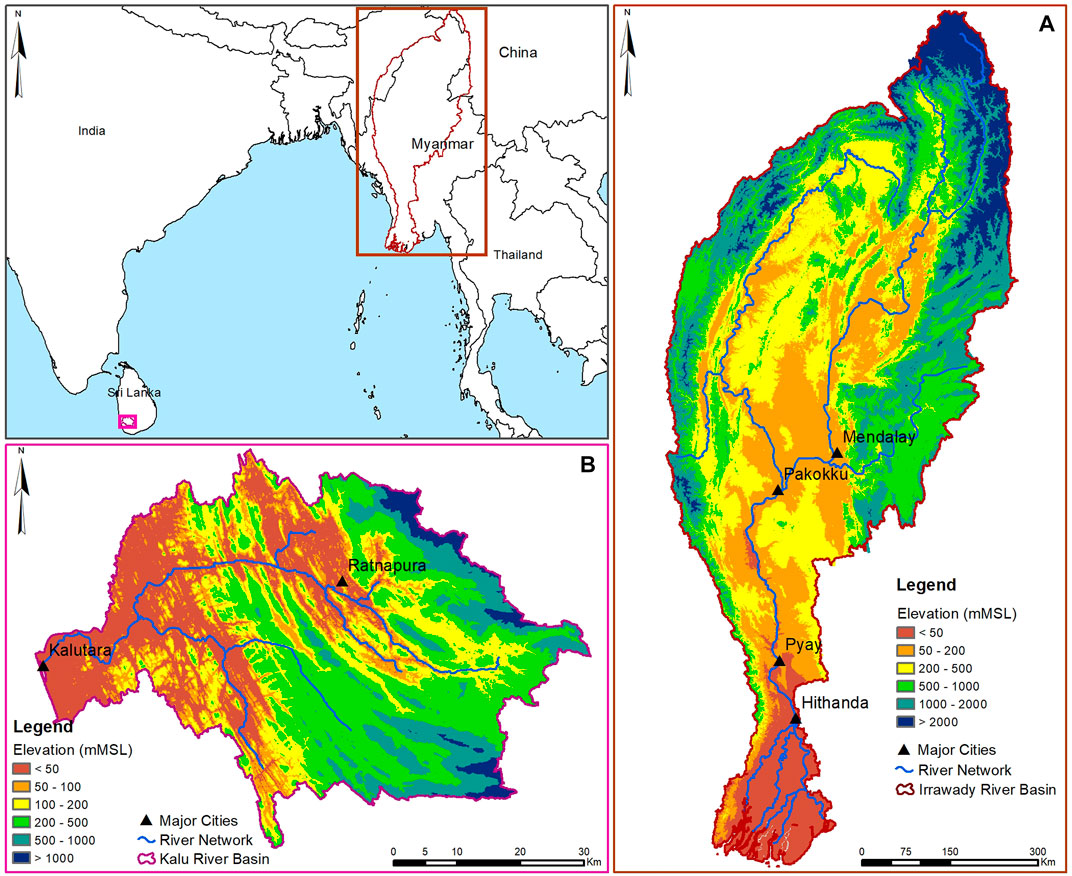
FIGURE 1. Irrawaddy river basin in Myanmar (A), Kalu river basin in Sri Lanka (B).

The Kalu River Basin is the second largest river basin in Sri Lanka and receives high rainfalls leading to high river flows. The Kalu River (Kalu Ganga) originates from the Samanala mountain range in the South-central part of Sri Lanka and falls out to the sea at Kaluthara after traversing ∼129 km (Figure 1B). The drainage area of the Kalu River is ∼2,787 km². The coastal zone adjacent to the Kalu river outfall comprises a small tidal inlet system experiencing a .6 m oceanic tidal range. Much of the basin is utilized for rain-fed paddy cultivation, rubber, tea, and other commercial crops scattered throughout the basin. Clay-rich Acrisol is the most dominant soil type found in the basin. The average annual rainfall in the basin is ∼3,800 mm, mainly driven by the southwest monsoon (May–September). The average daily temperature in the basin is ∼25°C. The Kalu river carries ∼4,000 Million m³ of water and ∼0.7 Million tons of sediment load annually (on average) to the sea.

2.2 The SWAT description and input data

The Soil Water Assessment Tool (SWAT), developed by USDA Agricultural Research Service (Arnold et al., 1998; Neitsch et al., 2011), is a process-based continuous-time model for catchment simulations. In SWAT, a river basin is partitioned into sub-basins and further divided into hydrological response units (HRUs) based on land use, soil type, and slope classes. HRUs are the primary computational units of SWAT. Major catchment processes modelled in SWAT are hydrology, soil erosion, nutrients/pesticides (water quality), plant growth, and channel routing. SWAT estimates the surface runoff of each HRU using the Soil Conservation Services-Curve Number (SCS-CN)(Soil Conservation Service, 1971; Soil Conservation Service Engineering Division, 1986) or the Green and Ampt infiltration method (Mein and Larson, 1973). In this study, the SCS-CN method was used in all the simulations. The model estimates the soil erosion at each HRU caused by rainfall and runoff using the Modified universal Soil Loss Equation (MUSLE) (Williams and Berndt, 1977; Wischmeier and Smith, 1978) and assumes that all eroded sediments reach the channels. MUSLE (Eq. 1) is the modified version of the Universal Soil Loss Equation (USLE). In this version, the rainfall energy factor in USLE is replaced with the runoff factor, which improves sediment predictions and allows for the simulation of individual storm events (Neitsch et al., 2011).

$sed=11.8\bullet {\left(Q_{surf}\bullet q_{peak}\bullet {area}_{hru}\right)}^{0.56}{K}_{USLE}\bullet C_{USLE}\bullet P_{USLE}\bullet {LS}_{USLE}\bullet CFRG(1)$

where, sed is the sediment yield (tons), $Q_{surf}$ is the surface runoff (mm), $q_{peak}$ is the peak runoff (m³/s), ${area}_{hru}$ is the area of HRU (ha), $K_{USLE}{,C}_{USLE},P_{USLE},and{LS}_{USLE}$ are USLE soil erodibility factor, cover, and management factor, support practice factor, and topographic factor, respectively, and $CFRG$ is the coarse fragment factor.

The sediment transport model used in SWAT consists of two processes (i.e., deposition and degradation) which determine the magnitude of sediment generated within a river reach. The amount of sediment deposition or degradation depends on several factors, such as the maximum sediment concentration transported with river flow (Eq. 2), according to Bagnold’s Equation (Neitsch et al., 2011), flow velocity, flow rate, soil cover, and erodibility of the reach.

${conc}_{sed,ch,mx}=c_{sp}\bullet v_{ch,pk}^{spexp}(2)$

where, ${conc}_{sed,ch,mx}$ is the maximum sediment concentration transported by water (ton/m³), $c_{sp}$ is the sediment transport coefficient; $v_{ch,pk}$ is the peak velocity in the river (m/s), and $spexp$ is the exponent of the velocity.

When the maximum sediment concentration that can be carried by the water flow is less than the sediment concentration of the reach, sediment deposition (Eq. 3) occurs and vice versa for sediment degradation (Eq. 4).

${sed}_{dep}=\left({conc}_{sed,ch,i}-{conc}_{sed,ch,mx}\right).V_{ch}(3)$

${sed}_{\mathit{deg}}=\left({conc}_{sed,ch,mx}-{conc}_{sed,ch,i}\right).V_{ch}\bullet K_{CH}\bullet C_{CH}(4)$

where, ${sed}_{dep}$ and ${sed}_{\mathit{deg}}$ are the deposited and reentratined sediment volumes in the reach, respectively (tons), ${conc}_{sed,ch,i}$ is the sediment concentration of the reach at the initial time (ton/m³), ${conc}_{sed,ch,mx}$ is the maximum sediment concentration, which can be carried by water (ton/m³), $V_{ch}$ is the water volume in the reach (m³), $K_{ch}$ is the erodibility factor of the channel, and $C_{CH}$ is the cover factor of the channel.

The amount of sediment (in tons) flowing out from a river reach (Eq. 5) is calculated based on the sediment amount (in tons–based on the initial amount of suspended sediment in the reach, deposited and degraded sediments), and volume of outflows.

${sed}_{out}={sed}_{ch}\bullet \frac{V_{out}}{V_{ch}}(5)$

where, ${sed}_{out}$ is the amount of sediment outflow from the reach (tons), ${sed}_{ch}$ is the suspended sediment load in the reach (tons), and $V_{out}$ is the outflow volume (m³).

As model inputs, SWAT requires surface elevation data (digital elevation model (DEM)), land use, soil characteristics, land management, and daily climatic data (i.e., precipitation, maximum and minimum temperatures). In this study, all the spatial data (i.e., DEM, landuse, and soil) were obtained from freely available global products. Hydro-meteorological data (i.e., precipitation, temperature, streamflow, and sediment load) were obtained from local authorities in the two countries (i.e., Myanmar and Sri Lanka) and previous studies and reports. The SWAT model setup for each basin was calibrated and validated for streamflow and sediment loads. At first, streamflow was calibrated and validated with the available data at eight stations in IRB and 3 stations in KRB. These models were subsequently calibrated and validated for sediment load at 3 stations in IRB and at the basin outlet of KRB. The detailed information on input data, calibration, and validation of the SWAT models for streamflow and sediment loads at the Irrawaddy and Kalu River Basins are presented in Sirisena et al., 2018, Sirisena et al., 2021a, and Sirisena et al., 2021b.

In SWAT simulations for future periods, precipitation and temperature data were obtained from three General Circulation Models (GCMs) for the Irrawaddy Basin and three Regional Climate Models (RCMs) for the Kalu Basin under RCP 2.6 and RCP 8.5. Here, simulations were performed for the two future periods considered (i.e., 2046–2065 (mid-century) and 2081–2100 (end-century)). The detailed descriptions of GCMs and RCMs are provided in Supplementary Table S1 and the selection of the respective GCMs and RCMs are summarized in Sirisena et al. (2021a), Sirisena et al. (2021b), respectively. It is assumed that prevailing land-use conditions will remain invariant throughout the modelling period, and the inclusion of planned reservoirs is the only future human activity considered. For the future periods, out of the several planned reservoirs in the Irrawaddy basin, six large reservoirs having capacities of 17.7, 2.2, 2.6, 11.2, 13.2, and 8.6 billion m³ were considered to analyze their impacts on streamflow and sediment transport using SWAT (more details can be found in Sirisena, 2020; Sirisena et al., 2021a). Each reservoir and its trapping efficiency are individually represented in the SWAT model.

2.3 The BQART model description and input data

Many coastal studies have used BQART presented by Syvitski and Milliman (2007) to project annual fluvial sediment supply to the coast (e.g. Balthazar et al., 2013; Bamunawala et al., 2018a; Bamunawala et al., 2020a; Bamunawala et al., 2020b; Bamunawala et al., 2021). BQART was developed using data from 488 global river basins, and it estimates the long-term average annual suspended sediment load using the following equations.

$Q_s=\omega B{Q}^{0.31}{A}^{0.5}RTforT\ge 2^{0}C(6)$

where Q_s is the sediment load in kg/s or MT/yr with ω = 0.02 or 0.0006, respectively, B is the lithology and human impact index, Q is the annual streamflow from the basin (km³/yr), A is the basin area (km²), R is the relief of the basin (km), T is mean annual temperature of the basin (^oC).

The term ‘B’ accounts for geology and human activities, which is defined as;

$B=IL\left(1-T_E\right)E_h(7)$

where I is the glacial erosion factor (I ≥ 1), L is the basin-wide lithology factor, $T_E$ is reservoir trapping efficiency, and $E_h$ is the human-induced erosion factor.

The term I is defined as

$I=1+0.09A_g(8)$

where, $A_g$ is the percentage of ice coverage area in the basin.

The main rivers in the two study areas are mostly in pristine condition. However, as mentioned earlier, six large planned reservoirs were considered in the hydrological simulations of the Irrawaddy basin. Since BQART is a lumped model, the trapping efficiency is defined for the entire basin. Therefore, for BQART applications, the basin-wide Trapping Efficiency (TE) from the six reservoirs was estimated using the method proposed by Vörösmarty et al. (2003) (from Eqs 6–11). Vörösmarty et al. (2003) developed the basin-wide trapping efficiency model for large reservoirs (>500 MCM) by considering 633 reservoir data across the world. This basin-wide trapping (${TE}_{basin}$) is derived by considering the geographical locations of the reservoirs and the sediment residence time from 236 regulated river basins. Figure 2 shows the schematic diagram of a representative basin as considered by Vörösmarty et al. (2003) in this derivation.

$∆{\tau }_{reg,j}=\frac{{\displaystyle \sum }_1^n{V}_i}{Q_j}\left(eg.\frac{\left(V_2+V_3+V_4+V_5\right)}{Q_B}\right)(9)$

${TE}_{reg,j}=1-\frac{0.05}{\sqrt{∆{\tau }_{reg,j}}}(10)$

${TE}_{basin}=\frac{{\displaystyle \sum }_1^m{TE}_{reg,j}{Q}_j}{Q_m}(11)$

where, $∆{\tau }_{reg,j}$ is the residence time of reservoir areas of j^th regulated sub-basin of the basin (j is A, B, and C here), $V_i$ is the operational volume of i^th reservoir in j, $Q_j$ is the discharge at regulated sub-basin j, ${TE}_{reg,j}$ is approximated trapping efficiencies of j^th sub-basin, ${TE}_{basin}$ is the discharge-weighted trapping efficiency of the basin based on discharge, $Q_m$ is discharge at the basin outlet, n is the number of reservoirs in each regulated sub-basin j, and m is the number of regulated sub-basins in the basin

FIGURE 2

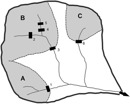
FIGURE 2. Vörösmarty et al. (2003)’s representation of a basin for estimating basin-wide sediment trapping for large reservoirs. Source - Vörösmarty et al. (2003). (A–C) are sub-basins.

For the Irrawaddy RB, different ${TE}_{basin}$ values were calculated for each General Circulation Model (GCM) under RCP 2.6 and RCP 8.5 for the two future periods considered (i.e., 2046–2065 (mid-century) and 2081–2100 (end-century)). Since there are no planned reservoirs for the Kalu basin, reservoir effects are not considered in the fluvial sediment load estimations. Furthermore, a zero trapping efficiency was considered while implementing the BQART model for both river basins to explicitly represent the climate-driven impacts on fluvial sediment supply. The calculation of ${TE}_{basin}$ (Eq. 11) is based on the volume of reservoirs, discharge from reservoirs, and discharge at the basin outlet. Based on three GCMs and two RCPs, the average basin-wide trapping efficiency (${TE}_{basin}$) of the Irrawaddy RB was computed as 42%. The river basin and reservoir data used by Vörösmarty et al. (2003) include some Asian River Basins, including Mekong (0%–20%), Chao-Pharya (20%–40%), Ganges and Brahmaputra (0%–20%), Krishna (80%–100%), Yangetz Basin (60%–80%), and Indus (40%–60%). The number of large reservoirs within each basin varies from 3–20. Furthermore, large reservoirs (633) and small reservoirs (>40,000) in the world contribute 30% and 23% of sediment trapping, respectively (Vörösmarty et al., 2003). Considering this wide range of computed trapping efficiencies, the above calculated ${TE}_{basin}$ of the Irrawaddy RB appears to be reasonable.

Table 1 summarizes the input parameters of the BQART model. The river discharge (Q) values were obtained from the SWAT simulation results presented in Sirisena, 2020; Sirisena et al., 2021a; Sirisena et al., 2021b over the baseline and mid-and end-century periods for RCP 2.6 and RCP 8.5. The mean temperature (T) over the basins was obtained from the three selected GCMs/RCMs (discussed in Sirisena et al., 2021a; Sirisena et al., 2021b for the same RCPs. The human-induced erosion factor ($E_h)$ in Eq. 7 is based on land use, socio-economic situation, and population density. The suggested optimum range of $E_h$ is 0.3 ≤ $E_h$ ≤ 2.0 (Syvitski and Milliman, 2007). Similar to the assumption made for the land-use change in SWAT simulations, for future simulations with the BQART model, the human-induced erosion factor ($E_h$) is assumed to remain constant throughout the 21st century (Table 1).

TABLE 1

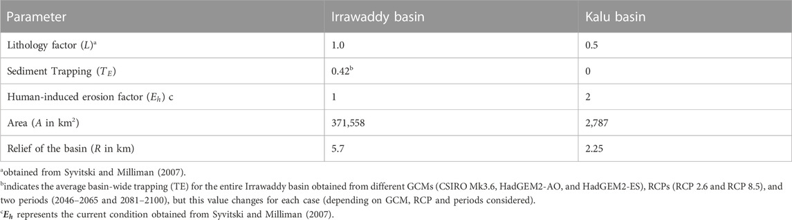
TABLE 1. Summary of model input parameters.

3 Results and discussion

3.1 Irrawaddy River Basin

3.1.1 Annual sediment fluxes to the coast simulated by BQART

BQART projected sediment loads at the basin outlet under different scenarios are presented in Figure 3 (Panel 1). The projected mean annual sediment loads for RCP 8.5 are higher than that of RCP 2.6 during both future periods considered. Sediment supply to the coast is projected to increase by 29%–41% (relative to the baseline period: 1991–2005) by the end-century (2081–2100) when the future changes are only due to climate change (RCP 8.5). In comparison, fluvial sediment supply is projected to decrease by 19%–24% due to the combined effect of climate change (RCP 8.5) and reservoirs during 2081–2100. The BQART projected sediment load varies between 319 and 356 MT/yr and between 326 and 412 MT/yr during mid-and end-century periods, respectively, under the assumed zero trapping condition (i.e., no reservoirs). These values are projected to reduce to 179–210 MT/yr and 189–247 MT/yr for the same two periods, respectively, when the reservoirs are considered (with basin-wide trapping efficiencies, see Methods). Due to the combined effects of climate change and reservoirs, the average reduction of sediment supply is about 41% for both future periods relative to that due to climate change alone. Therefore, it is evident that the basin-wide trapping $\left({TE}_{basin}\right)$ is the main influencing factor ($T_E$ = 0.42; Table 1) for this reduction.

FIGURE 3

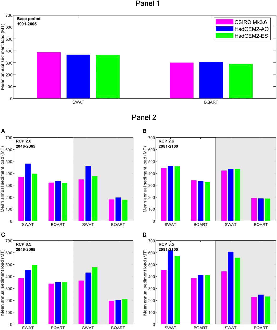
FIGURE 3. Comparison of the mean annual sediment projections (Millions Tons (MT)) at the Irrawaddy basin outlet obtained from SWAT and BQART. Panel 1 shows the estimates of sediment loads for the baseline period (1991–2005) and Panel 2 shows two future periods (2046-2065 and 2081–2100) under two RCPs (RCP 2.6 (A,B) and 8.5 (C,D), respectively. The shaded area in Panel 2 represents the results under CC + Reservoirs scenario.

3.1.2 Comparison of SWAT and BQART projected sediment loads: The Irrawaddy basin outlet

The SWAT model setup and sediment load projections at the IRB are described in detail in Sirisena et al. (2018) and Sirisena et al. (2021b). Therefore, only a summary is presented in Methods. The SWAT-derived baseline period and future projections of sediment loads at the Irrawaddy RB outlet are consistently higher than that obtained from BQART for all three GCMs considered (Figure 3). For the baseline period (1991–2005), simulated mean sediment loads from SWAT and BQART are 365–388 MT/yr and 290–307 MT/yr, respectively (Figure 3-Panel 1). These simulated values are obtained for three GCMs (viz., CSIRO Mk3.6, HadGEM2-AO, and HadGEM2-ES). The BQART-derived sediment load values for the baseline period are 17%–23% lower than those derived from SWAT for the same period. Syvitski and Milliman (2007) have calculated the average sediment yield in the Irrawaddy RB as 258.6 MT/yr with input parameters of Q = 13,560 m³/s, A = 405,963 km², R = 4.8 km, and T = 22°C based on previous studies by Milliman and Meade (1983), Milliman and Syvitski (1992), and Syvitski (2003), which is not too different from the BQART prediction obtained here, considering the level of aggregation in the model.

During the mid-century period (2046–2065, Figure 3A-Panel 2, the BQART projections are 13%–30% and 48%–57% lower than the SWAT projections under RCP 2.6 without and with reservoirs, respectively. Those values under RCP 8.5 are 12%–28% and 46%–56% for without and with reservoirs, respectively (Figure 3C-Panel 2). Similarly, during the end-century period, BQART projections are 23%–29% and 54%–57% lower than the SWAT projections under RCP 2.6 for simulations without and with reservoirs, respectively (Figure 3B-Panel 2). Under RCP 8.5, those BQART projections are 15%–33% (without reservoirs) and 49%–59% (with reservoirs) lower than SWAT projections (Figure 3D-Panel 2).

In general, BQART projections show smaller increments with climate change only and a higher reduction of sediment loads with reservoirs (relative to the baseline period) compared to the corresponding SWAT-derived projections, except for the SWAT simulation driven by CSIRO Mk3.6 (Figure 4). With climate change alone, during the mid-century period, SWAT and BQART model projections indicate changes in sediment load by -5%–31% and 7%–10% under RCP 2.6, respectively (compared to the baseline period, Figure 4A). The same projections under RCP 8.5 are -1%–36% (with SWAT) and 13%–23% (with BQART) (Figure 4C). Similarly, SWAT and BQART model projections indicate increases in sediment load by 14%–25% and 9%–13% under RCP 2.6, respectively, during the end-century period (Figure 4B). Under RCP 8.5 for the same period (Figure 4D), SWAT and BQART projections show increments of 17%–66% and 29%–41%, respectively. In contrast, with planned reservoirs, under RCP 2.6, BQART projects sediment load reductions of 35%–40% and 35%–38% during mid-and end-century periods, respectively (compared to the baseline period). The same BQART projections under RCP 8.5 are 27%–34% (mid-century) and 19%–24% (end-century). On the contrary, SWAT projections indicate increases of sediment loads by -10%–25% (mid-century) and 9%–20% (end-century) under RCP 2.6. Similarly, under RCP8.5, the SWAT simulations indicate -6%–31% (mid-century) and 9%–20% (end-century) variations in sediment loads supplied to the coast. Such directional changes in the projections obtained from the two models are a serious cause for concern, especially when used in reduced complexity modelling approaches to assess future coastline variations.

FIGURE 4

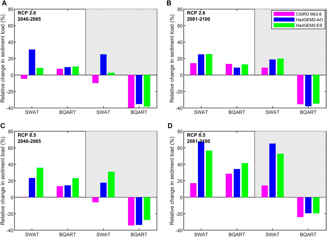
FIGURE 4. Comparison of the relative changes in mean annual sediment projections under RCP 2.6 (A, B) and RCP 8.5 (C, D) for future periods (2046–2065 and 2081–2100) compared to the baseline period model estimates at the Irrawaddy basin outlet using SWAT and BQART. The shaded area in each plot represents results under CC + Reservoirs scenario. The positive changes (+%) mean that the sediment load is projected to increase in the future compared to the baseline period, while negative changes (- %) mean that the sediment load is projected to decrease.

There could be several reasons for these significant mismatches between the two models. BQART uses the mean annual streamflow and thus does not differentiate the inter-annual variability in sediment load. On the other hand, SWAT simulates daily time steps, thus accounting for both high and low flow conditions. SWAT simulations provide the total sediment load at the basin outlet for a given year. It is based on the sediment erosion within the basin and sediment routing through the river reaches. Another distinction between SWAT and BQART is in the use of temperature data. BQART computes the sediment load as a linear function of the basin’s mean annual temperature. Furthermore, the mean annual temperatures used in BQART are not bias-corrected, and these raw GCM temperature projections may underestimate the basin-wide temperature (see Materials and methods section). All these factors may have contributed to the lower sediment load estimates given by BQART. A significant difference (up to 53%) in sediment load projections obtained from the two models can be seen in simulations that account for planned reservoirs. Such differences may have occurred due to the estimated basin-wide trapping efficiency used in BQART as opposed to reservoir-specific TEs used in SWAT. Based on the calculated basin-wide trapping efficiency, approximately 42% of the sediment load is expected to be trapped by the reservoirs. However, no records are available to verify this value for the Irrawaddy basin.

3.2 Kalu river basin

3.2.1 Comparison of SWAT and BQART projected sediment loads: The Kalu basin outlet

Detailed descriptions of the SWAT model setup and simulated sediment load projections at the KRB are presented in Sirisena (2020) and Sirisena et al. (2021a). A comparison of the above BQART projections with the results obtained using SWAT (under the same conditions) is shown in Figure 5. Here, the BQART projections of sediment load at the basin outlet are up to an order of magnitude larger than that of the SWAT simulation results. For the baseline period (Figure 5-Panel 1), SWAT and BQART respectively simulate 0.63–0.66 MT/yr and 2.72–2.75 MT/yr of sediment load with inputs from 3 RegCM4 RCMs. During the end-century period, the BQART model projections are 234%–281% and 116%–145% higher than the SWAT simulations for RCP 2.6 and RCP 8.5, respectively (Figure 5B–D-Panel 2).

FIGURE 5

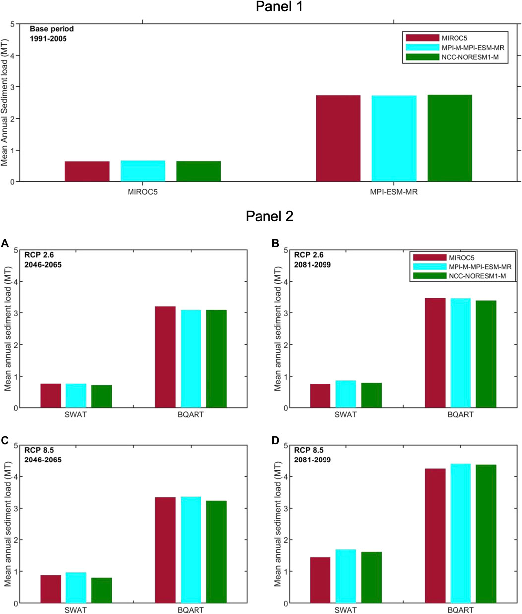
FIGURE 5. Comparison of the mean annual sediment projections (Million tons (MT)) at the Kalu basin outlet obtained from SWAT and BQART. Panel 1 shows the estimated sediment loads for the baseline period (1991–2005) and Panel 2 shows two future periods (2046–2065 and 2081–2099) under two RCPs (RCP 2.6 (A,B) and RCP 8.5 (C,D), respectively.

In general, during both future periods, the SWAT simulations show higher increments of sediment loads under both RCPs (Figure 6). For example, during the end-century period, SWAT and BQART project increased sediment load by 20%–32% and 3%–6% under RCP 2.6, respectively. For RCP 8.5, the SWAT and BQART projected increases in sediment loads are 128%–158% and 30%–35%, respectively. All these changes are calculated relative to the baseline period simulations of the respective models. Less increment in sediment load projections by BQART (compared to SWAT projections) relative to the baseline period is likely due to its low sensitivity to streamflow. In BQART model, the streamflow is associated with a power of 0.31. Thus, for example, a 10 times increase in streamflow will only result in ∼2 times increase in sediment load projection with the BQART model. Here, streamflow is projected to increase by 67%–87% under RCP 8.5 by the end century. However, such significant increases in streamflow will have considerable implications on increasing the SWAT projected sediment loads.

FIGURE 6

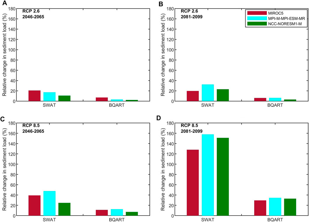
FIGURE 6. Comparison of the relative changes of mean annual sediment projections under RCP 2.6 (A, B) and RCP 8.5 (C, D) for future periods (2046–2065 and 2081–2099) compared to the baseline period model estimates at the Kalu basin outlet using SWAT and BQART. The positive changes (+%) mean that sediment load is projected to increase in the future compared to the baseline period.

One explanation for the significant differences between the sediment loads projected by the two models could be the use of the aggregated quantity human-induced erosion factor $\left(E_h\right)$ in BQART. This factor is based on countrywide GNP/capita (Gross Net Product per capita) and population density. Hence using the value for all of Sri Lanka, by following Syvitski and Milliman (2007), an $E_h$ value of 2.0 was used in the calculations for the Kalu River Basin. However, as the Kalu River Basin contains large areas of forest reserves and settlements of low-income communities, this $E_{\mathrm{h}}$ value is likely to be a different value.

3.3 BQART projections with updated E_h values

The parameter ‘B’ in the BQART represents the geology and human activities in the basin. The human-induced erosion factor ($E_h)$ is one of the main influencing factors and is linearly correlated with B and consequently with the fluvial sediment load computed by BQART; Syvitski and Milliman (2007) have derived the $E_h$ factor based on land use, socio-economic situation and population. However, recent studies by Balthazar et al. (2013); Bamunawala et al., 2020b; Bamunawala et al., 2020a; Bamunawala et al., 2021 have shown that the human footprint index (HFPI) presented by Wildlife Conservation Society-WCS and Center for International Earth Science Information Network-CIESIN-Columbia University (2005) can be a better representation of the anthropogenic influences on fluvial sediment load estimation via BQART. The HFPI was developed based on several global datasets, including population, urban areas, land use, navigable waterways, roads, and electrical infrastructure (Sanderson et al., 2002).

As a further test of SWAT and BQART projected fluvial sediment loads, the BQART projections were re-calculated with the updated $E_h$ (using HFPI) and re-compared with the corresponding SWAT projections. To do this, HFPI values, which range from 0–100, need to be rescaled to the global range of $E_h$ (0.3 ≤ $E_h$ ≤ 2.0) estimated by Syvitski and Milliman (2007) for use in the BQART. HFPI values across the Irrawaddy and Kalu River Basins were obtained from 0.25° × 0.25° resolution data (Wildlife Conservation Society-WCS and Center for International Earth Science Information Network-CIESIN-Columbia University, 2005) and rescaled accordingly. Subsequently, the basin average rescaled HFPI values were used with BQART to re-compute the fluvial sediment load at the outlets of the two basins. The comparison of projected sediment loads from SWAT and BQART (with the two different $E_h$ factors; one derived from HFPI and one following Syvitski and Milliman (2007) with climate change only (i.e., no reservoirs) is shown in Table 2. With the HFPI-based $E_h$, BQART projects lower sediment loads in both basins than its previous estimations. This is because the HFPI-based human-induced erosion factors $\left(E_h\right)$ for the two basin areas are almost half the $E_h$ values suggested by Syvitski and Milliman (2007) (Table 1).

TABLE 2

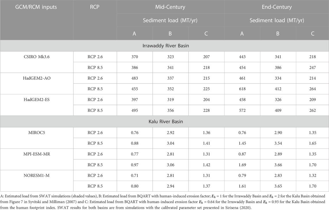
TABLE 2. Projected average annual sediment loads in Million tons per year (MT/yr) for the Irrawaddy and Kalu basins under RCP 2.6 and RCP 8.5, without reservoirs.

3.4 Comparison of the modelled results in the two basins

The sediment load projections by SWAT and BQART are different in the two river basins. In Irrawaddy RB, SWAT simulations project a higher sediment load than those predicted by BQART and vice versa in the Kalu RB. For example, when using the human-induced erosion factor ($E_h$) obtained from Syvitski and Milliman (2007), for the baseline period (1991–2005), simulated sediment loads by the models differ by 18%–22% in the Irrawaddy RB and 315%–331% in the Kalu RB. During the end-century period under RCP 8.5, those differences in projected sediment loads are 15%–33% in the Irrawaddy RB and 116%–145% in the Kalu RB. During the same period and under the same RCP, the projected sediment supply is further reduced in the Irrawaddy RB due to the proposed reservoirs. Therefore, the difference in sediment loads between BQART and SWAT projections is 48%–59%. Compared to the baseline period (1991–2005) model estimations, BQART projections generally show lower increments than SWAT projected increments in the Irrawaddy and Kalu River Basins when the reservoirs are not considered (i.e., climate change only).

When adopting the human-induced erosion factor ($E_h$) derived from the human footprint index (HFPI), the baseline period (1991–2005) projected sediment loads by BQART and SWAT differ by 46%–50% and 93%–101% in the Irrawaddy RB and the Kalu RB, respectively. For the end-century period under RCP 8.5, those differences in the sediment load projections are 70%–72% and 1%–14% in the Irrawaddy RB and the Kalu RB, respectively.

BQART does not provide information on sediment erosion, transport, and deposition in the flood plains, as it only estimates the sediment delivery rate at/near sea level of the basin outlet (Syvitski and Milliman, 2007). The empirical BQART equation is developed based on 488 global river datasets comprising catchments sizes spanning a large range (160 km²–5,853,804 km²) with high accuracy in calibration (R² = 0.96 for 292 basins) and validation (R² = 0.94 for 196 basins) (Syvitski and Milliman, 2007). However, an analysis by De Vente et al. (2013) summarized that non-linear regression models like BQART might provide more accurate results than distributed models such as SWAT would for sediment yield in basins larger than 10,000 km². Nevertheless, a study of the Blue Nile and Atbara river systems showed that a global flux model such as BQART is less suited for capturing highly spatially varied sediment yields ranging from thousands of ton/km²/year in a basin (Balthazar et al., 2013). Although, spatially distributed models such as SWAT demand more input data and high calibration efforts they are more suitable for assessing environmental change scenarios such as those due to climate change, land use, and management practices (Neitsch et al., 2011). Therefore, both models have their advantages and disadvantages in sediment load estimation for a selected region under diverse environmental and geographical conditions.

4 Conclusion

This study aimed to estimate fluvial sediment supply to the coast using a distributed process-based model (SWAT) and an empirical lumped model (BQART) in the Irrawaddy River (Myanmar) and Kalu River (Sri Lanka) Basins. Similar to the SWAT simulations described in Sirisena (2020), the BQART simulations were undertaken with and without reservoirs over the two future periods considered (i.e., 2046–2065 and 2081–2100) for the RCP 2.6 and 8.5.

Our results show significant differences between the sediment loads projected by the two models in the two basins. In the Irrawaddy River Basin, SWAT simulations project higher sediment loads than BQART. In contrast, SWAT simulations project lower sediment loads than BQART projections in the Kalu River Basin. For both future periods, relative to the baseline period (1991–2005), BQART-derived projections show lower future increases than SWAT in both basins with climate change alone (i.e., no reservoirs). Our results also indicate that empirical BQART model-based projections are more in line with the semi-distributed SWAT model-based projections in the larger Irrawaddy RB than in the smaller Kalu RB.

Both SWAT and BQART model projections possess considerable variabilities due to the inherent uncertainties in projected future climatic inputs (i.e., precipitation and temperature) and other variables such as human-induced erosion factor and model calibration parameters. An aggregated global model such as the BQART does not always guarantee equally good results in all regions, as it is not explicitly calibrated for individual study regions. SWAT, as a standard practice, is calibrated to the specific basin, thus, the quality of SWAT model results also depends on the quality/quantity of data available for calibration. On the other hand, reservoir simulation with SWAT requires detailed information, such as operational capacity, high flood level, operation rules/practices, and sediment data. In practice, some of these reservoir-specific information/data are often unavailable, and approximations are commonly used. Thus, both model approaches adopt certain approximations, adding to the uncertainty of the projected sediment loads.

Data availability statement

The raw data supporting the conclusion of this article will be made available by the authors without undue reservation Requests to access these datasets should be directed to TS, jeewanthisri@gmail.com.

Author contributions

TS carried out the design, model simulations, and drafting of the manuscript. JB assisted with GCM data collection and analysis and collection of BQART parameters. SM and RR guided the methodology development. All authors provided feedback on the manuscript.

Funding

This study is a part of TS’s research, supported by the EPP Myanmar project and Netherlands Fellowship Programme (NFP).

Acknowledgments

TS is supported by the EPP Myanmar project and Netherlands Fellowship Programme (NFP). RR is supported by the AXA Research Fund and the Deltares Strategic Research Programme ‘Coastal and Offshore Engineering’. Last of the Wild Project, Global Human Footprint, Version 2 data were developed by the Wildlife Conservation Society—WCS and the Center for International Earth Science Information Network (CIESIN), Columbia University and were obtained from the NASA Socioeconomic Data and Applications Center (SEDAC) at http://dx.doi.org/10.7927/H4M61H5F. Accessed 1 November 2018.

Conflict of interest

The authors declare that the research was conducted in the absence of any commercial or financial relationships that could be construed as a potential conflict of interest.

Publisher’s note

All claims expressed in this article are solely those of the authors and do not necessarily represent those of their affiliated organizations, or those of the publisher, the editors and the reviewers. Any product that may be evaluated in this article, or claim that may be made by its manufacturer, is not guaranteed or endorsed by the publisher.

Supplementary material

The Supplementary Material for this article can be found online at: https://www.frontiersin.org/articles/10.3389/feart.2022.978109/full#supplementary-material

References

Arnold, J. G., Srinivasan, R., Muttiah, R. S., and Williams, J. R. (1998). Large area hydrologic modeling and assessment Part I: Model development. JAWRA J. Am. Water Resour. Assoc. 34, 73–89. doi:10.1111/j.1752-1688.1998.tb05961.x

CrossRef Full Text | Google Scholar

Balthazar, V., Vanacker, V., Girma, A., Poesen, J., and Golla, S. (2013). Human impact on sediment fluxes within the Blue nile and Atbara River basins. Geomorphology 180–181, 231–241. doi:10.1016/j.geomorph.2012.10.013

PubMed Abstract | CrossRef Full Text | Google Scholar

Bamunawala, J., Dastgheib, A., Ranasinghe, R., Spek, A. van der, Maskey, S., Duong, T. M., et al. (2020a). A holistic modeling approach to project the evolution of inlet-interrupted coastlines over the 21st century. Front. Mar. Sci. 7, 542–620. doi:10.3389/fmars.2020.00542

CrossRef Full Text | Google Scholar

Bamunawala, J., Dastgheib, A., Ranasinghe, R., Spek, A. Van Der, Murray, A. B., Barnard, P. L., et al. (2020b). Acidification in the U S. Southeast: Causes, potential consequences and the role of the Southeast ocean and coastal acidification Network. Front. Mar. Sci. 7, 1–548. doi:10.3389/fmars.2020.00548

PubMed Abstract | CrossRef Full Text | Google Scholar

Bamunawala, J., Maskey, S., Duong, T., and van der Spek, A. (2018a). Significance of fluvial sediment supply in coastline modelling at tidal inlets. J. Mar. Sci. Eng. 6, 79–12. doi:10.3390/jmse6030079

CrossRef Full Text | Google Scholar

Bamunawala, J., Ranasinghe, R., Dastgheib, A., Nicholls, R. J., Murray, A. B., Barnard, P. L., et al. (2021). Twenty-first-century projections of shoreline change along inlet-interrupted coastlines. Sci. Rep. 11, 14038–14114. doi:10.1038/s41598-021-93221-9

PubMed Abstract | CrossRef Full Text | Google Scholar

Bamunawala, J., Ranasinghe, R., van der Spek, A., Maskey, S., and Udo, K. (2018b). Assessing future coastline change in the vicinity of tidal inlets via reduced complexity modelling. J. Coast. Res. 85, 636–640. doi:10.2112/si85-128.1

CrossRef Full Text | Google Scholar

Besset, M., Anthony, E. J., and Bouchette, F. (2019). Multi-decadal variations in delta shorelines and their relationship to river sediment supply: An assessment and review. Earth-Science Rev. 193, 199–219. doi:10.1016/j.earscirev.2019.04.018

CrossRef Full Text | Google Scholar

Bingner, R.-R., and Theurer, F. (2001). “AnnAGNPS: Estimating sediment yield by particle size for sheet and rill erosion,” in Sediment: Monitoring, modeling, and managing, 7th federal interagency sedimentation conference. Subcommittee on sedimentation interagency advisory committee on water data (Reno, NV, U S, I. 7)).

Google Scholar

Cohen, S., Kettner, J. a., Syvitski, J. P. M., and Fekete, B. M. (2013). WBMsed, a distributed global-scale riverine sediment flux model: Model description and validation. Comput. Geosci. 53, 80–93. doi:10.1016/j.cageo.2011.08.011

CrossRef Full Text | Google Scholar

De Roo, A. P. J., Wesseling, C. G., and Ritsema, C. J. (1996). Lisem: A single-event physically based hydrological and soil erosion model for drainage basins. I: Theory, input and output Hydrol. Process., 10, 11072–11174. doi:10.1002/(SICI)1099-1085

CrossRef Full Text | Google Scholar

De Vente, J., Poesen, J., Verstraeten, G., Govers, G., Vanmaercke, M., Van Rompaey, A., et al. (2013). Predicting soil erosion and sediment yield at regional scales: Where do we stand? Earth-Science Rev. 127, 16–29. doi:10.1016/j.earscirev.2013.08.014

CrossRef Full Text | Google Scholar

De Vente, J., Poesen, J., Verstraeten, G., and RompaeyAnton Van Govers, G. (2008). Spatially distributed modelling of soil erosion and sediment yield at regional scales in Spain. Glob. Planet. Change 60, 393–415. doi:10.1016/j.gloplacha.2007.05.002

CrossRef Full Text | Google Scholar

Dunn, F. E., Darby, S. E., Nicholls, R. J., Cohen, S., Zarfl, C., and Fekete, B. M. (2019). Projections of declining fluvial sediment delivery to major deltas worldwide in response to climate change and anthropogenic stress. Environ. Res. Lett. 14, 084034. doi:10.1088/1748-9326/ab304e

CrossRef Full Text | Google Scholar

Dunn, F. E., Nicholls, R. J., Darby, S. E., Cohen, S., Zarfl, C., and Fekete, B. M. (2018). Projections of historical and 21st century fluvial sediment delivery to the Ganges-Brahmaputra-Meghna, Mahanadi, and Volta deltas. Sci. Total Environ. 642, 105–116. doi:10.1016/j.scitotenv.2018.06.006

PubMed Abstract | CrossRef Full Text | Google Scholar

Kirkby, M. J., Irvine, B. J., Jones, R. J. A., Govers, G., and Team, P. (2008). The PESERA coarse scale erosion model for Europe. I. Model rationale and implementation. Eur. J. Soil Sci. 59, 1293–1306. doi:10.1111/j.1365-2389.2008.01072.x

CrossRef Full Text | Google Scholar

McGranahan, G., Balk, D., and Anderson, B. (2007). The rising tide: Assessing the risks of climate change and human settlements in low elevation coastal zones. Environ. Urban. 19, 17–37. doi:10.1177/0956247807076960

CrossRef Full Text | Google Scholar

Mein, R ., and Larson, C. (1973). Modeling infiltration during a steady rain. Water Resour. Res. 9, 384–394. doi:10.1029/wr009i002p00384

CrossRef Full Text | Google Scholar

Merkens, J.-L., Reimann, L., Hinkel, J., and Vafeidis, A. T. (2016). Gridded population projections for the coastal zone under the Shared Socioeconomic Pathways. Glob. Planet. Change 145, 57–66. doi:10.1016/j.gloplacha.2016.08.009

CrossRef Full Text | Google Scholar

Miao, C., Ni, J., Borthwick, A. G. L., and Yang, L. (2011). A preliminary estimate of human and natural contributions to the changes in water discharge and sediment load in the Yellow River. Glob. Planet. Change 76, 196–205. doi:10.1016/j.gloplacha.2011.01.008

CrossRef Full Text | Google Scholar

Milliman, J. D., and Meade, R. H. (1983). World-wide delivery of river sediment to the oceans. J. Geol. 91, 1–21. doi:10.1086/628741

CrossRef Full Text | Google Scholar

Milliman, J. D., and Syvitski, J. P. M. (1992). Geomorphic/tectonic control of sediment discharge to the ocean: The importance of small mountainous rivers. J. Geol. 100, 525–544. doi:10.1086/629606

CrossRef Full Text | Google Scholar

Neitsch, S. L., Arnold, J. G., Kiniry, J. R., and Williams, J. R. (2011). Soil and water assessment Tool theoretical documentation version 2009. Texas, U S: Texas Water Resources Institute. doi:10.1016/j.scitotenv.2015.11.063

CrossRef Full Text | Google Scholar

Neumann, B., Vafeidis, A. T., Zimmermann, J., and Nicholls, R. J. (2015). Future coastal population growth and exposure to sea-level rise and coastal flooding - a global assessment. PLoS One 10, e0118571. doi:10.1371/journal.pone.0118571

PubMed Abstract | CrossRef Full Text | Google Scholar

Nicholls, R. J., Wong, P. P., Burkett, V., Woodroffe, C. D., and Hay, J. (2008). Climate change and coastal vulnerability assessment: Scenarios for integrated assessment. Sustain. Sci. 3, 89–102. doi:10.1007/s11625-008-0050-4

CrossRef Full Text | Google Scholar

Nicholls, R. J., Woodroffe, C. D., Burkett, V., Hay, J., Wong, P. P., and Nurse, L. (2011). “Scenarios for coastal vulnerability assessment,” in Treatise on estuarine and coastal science. Editors E. Wolanski, D. B. T.-T. on E., and C. S. McLusky (Cambridge, MA, U S: Academic Press), 289–303. doi:10.1016/B978-0-12-374711-2.01217-1

CrossRef Full Text | Google Scholar

Oppenheimer, M., Glavovic, B. C., Hinkel, J., Van-de-Wal, R., Magnan, A. K., Abd-Elgawad, A., et al. (2019). “Sea level rise and implications for low-lying islands, coasts and communities,” in IPCC special report on the ocean and cryosphere in a changing climate. H.-O. Pörtner, D. C. Roberts, V. Masson-Delmotte, P. Zhai, M. Tignor, E. Poloczanskaet al. (In Press).

Google Scholar

Overeem, I., and Syvitski, J. P. M. (2009). Dynamics and vulnerability of delta systems. LOICZ reports & studies No. 35. Geesthacht, Germany: GKSS Research Center.

Google Scholar

Pelletier, J. D. (2012). A spatially distributed model for the long-term suspended sediment discharge and delivery ratio of drainage basins. J. Geophys. Res. Earth Surf. 117, 1–15. doi:10.1029/2011JF002129

CrossRef Full Text | Google Scholar

Ranasinghe, R., Duong, T. M., Uhlenbrook, S., Roelvink, D., and Stive, M. (2012). Climate-change impact assessment for inlet-interrupted coastlines. Nat. Clim. Chang. 3, 83–87. doi:10.1038/NCLIMATE1664

CrossRef Full Text | Google Scholar

Ranasinghe, R. (2020). On the need for a new generation of coastal change models for the 21st century. Sci. Rep. 10, 2010–2016. doi:10.1038/s41598-020-58376-x

PubMed Abstract | CrossRef Full Text | Google Scholar

Ranasinghe, R., Wu, C. S., Conallin, J., Duong, T. M., and Anthony, E. J. (2019). Disentangling the relative impacts of climate change and human activities on fluvial sediment supply to the coast by the world ’s large rivers: Pearl River Basin, China. Sci. Rep. 9, 9236–9310. doi:10.1038/s41598-019-45442-2

PubMed Abstract | CrossRef Full Text | Google Scholar

Rodolfo, K. (1975). “The Irrawaddy delta: Tertiary setting and modern offshore sedimentation. The Irrawaddy delta: Tertiary setting and modern Offshore sedimentation,” in Deltas: Models for exploration. Editor M. L. Broussard (Houston, TX, U S: Houston Geological Society), 339–356.

Google Scholar

Rompaey, A. J. J. Van, Verstraeten, G., Oost, K. Van, Govers, G., and Poesen, J. (2001). Modelling mean annual sediment yield using a distributed approach. Earth Surf. Process. landforms 26, 1221–1236. doi:10.1002/esp.275

CrossRef Full Text | Google Scholar

Sanderson, E. W., Jaiteh, M., Levy, M. A., Redford, K. H., Wannebo, A. V., and Woolmer, G. (2002). The human footprint and the last of the Wild. Bioscience 52, 891–904. doi:10.1641/0006-3568(2002)052[0891:thfatl]2.0.co;2

CrossRef Full Text | Google Scholar

Sirisena, T. A. J. G., Maskey, S., Bamunawala, J., Coppola, E., and Ranasinghe, R. (2021a). Projected streamflow and sediment supply under changing climate to the coast of the Kalu river basin in tropical Sri Lanka over the 21st century WaterSwitzerl., 13.3031 doi:10.3390/w13213031

CrossRef Full Text | Google Scholar

Sirisena, T. A. J. G., Maskey, S., Bamunawala, J., and Ranasinghe, R. (2021b). Climate change and reservoir impacts on 21st century streamflow and fluvial sediment loads in the Irrawaddy River, Myanmar. Front. Earth Sci. Hydrosph. 9, 644527–644616. doi:10.3389/feart.2021.644527

CrossRef Full Text | Google Scholar

Sirisena, T. A. J. G., Maskey, S., Ranasinghe, R., and Babel, S. (2018). Effects of different precipitation inputs on streamflow simulation in the Irrawaddy River Basin, Myanmar. J. Hydrol. Reg. Stud. 19, 265–278. doi:10.1016/j.ejrh.2018.10.005

CrossRef Full Text | Google Scholar

Sirisena, T. A. J. G. (2020). Process based modelling of future variations in river flows and fluvial sediment supply to coasts due to climate change and human activities: Data poor regions. Doctor of Philosophy. Enschede, Netherlands: University of Twente.

Google Scholar

Soil Conservation Service Engineering Division (1986). Urban hydrology for small watersheds. Riverdale, MD, U S: U.S. Department of Agriculture.

Google Scholar

Soil Conservation Service (1971). “Section 4: Hydrology,” in National engineering handbook. Minneapolis, Minnesota: University of Minnesota.

Google Scholar

Syvitski, J. P. M., Kettner, A. J., Overeem, I., Hutton, E. W. H., Hannon, M. T., Brakenridge, G. R., et al. (2009). Sinking deltas due to human activities. Nat. Geosci. 2, 681–686. doi:10.1038/ngeo629

CrossRef Full Text | Google Scholar

Syvitski, J. P. M., and Milliman, J. D. (2007). Geology, geography, and humans battle for dominance over the delivery of fluvial sediment to the coastal ocean. J. Geol. 115, 1–19. doi:10.1086/509246

CrossRef Full Text | Google Scholar

Syvitski, J. P. M., Peckham, S. D., Hilberman, R., and Mulder, T. (2003). Predicting the terrestrial flux of sediment to the global ocean: A planetary perspective. Sediment. Geol. 162, 5–24. doi:10.1016/S0037-0738(03)00232-X

CrossRef Full Text | Google Scholar

Syvitski, J. P. M. (2003). Supply and flux of sediment along hydrological pathways: Research for the 21st century. Glob. Planet. Change 39, 1–11. doi:10.1016/S0921-8181(03)00008-0

CrossRef Full Text | Google Scholar

Syvitski, J. P. M., Vörösmarty, C. J., Kettner, Ka. J., and Green, P. (2005). Impact of humans on the flux of terrestrial sediment to the global coastal ocean. Sci. 308, 376–380. doi:10.1126/science.1109454

PubMed Abstract | CrossRef Full Text | Google Scholar

Vafeidis, A., Neumann, B., Zimmermann, J., and Nicholls, R. J. (2011). “MR9: Analysis of land area and population in the low-elevation coastal zone (LECZ),” in UK government’s foresight project (London, UK: Migration and Global Environmental Change), 172.

Google Scholar

Vörösmarty, C. J., Meybeck, M., Fekete, B., Sharma, K., Green, P., and Syvitski, J. P. M. (2003). Anthropogenic sediment retention: Major global impact from registered river impoundments. Glob. Planet. Change 39, 169–190. doi:10.1016/S0921-8181(03)00023-7

CrossRef Full Text | Google Scholar

Walling, D. E. (2009). The impact of global change on erosion and sediment transport by rivers: Current progress and future challenges. New York, NY, USA: Sprinker.

Google Scholar

Wildlife Conservation Society-WCS, and Center for International Earth Science Information Network-CIESIN-Columbia University (2005). Last of the Wild project, version 2, 2005 (LWP-2): Global human footprint dataset (geographic). Palisades, NY, USA: NASA Socioeconomic Data and Applications Center. doi:10.7927/H4M61H5F

CrossRef Full Text | Google Scholar

Williams, J. R., and Berndt, H. (1977). Sediment yield prediction based on watershed hydrology. Trans. Am. Soc. Agric. Eng. 20, 1100–1104. doi:10.13031/2013.35710

CrossRef Full Text | Google Scholar

Wischmeier, W. H., and Smith, D. D. (1978). Predicting rainfall erosion losses. Riverdale, MD, USA: U.S. Department of Agriculture. doi:10.1029/TR039i002p00285

CrossRef Full Text | Google Scholar

Wong, P. P., Losada, I. J., Gattuso, J.-P., Hinkel, J., Khattabi, A., McInnes, K. L., et al. (2014). “Coastal systems and low-lying areas,” in Climate change 2014: Impacts, adaptation, and vulnerability. Part A: Global and sectoral aspects. Contribution of working group II to the fifth assessment report of the intergovernmental Panel on climate change. C. B. Field, V. R. Barros, D. J. Dokken, K. J. Mach, M. D. Mastrandrea, T. E. Biliret al. (Cambridge, UK: Cambridge University Press), 361–409.

Google Scholar

Yang, S. L., Xu, K. H., Milliman, J. D., Yang, H. F., and Wu, C. S. (2015). Decline of Yangtze River water and sediment discharge: Impact from natural and anthropogenic changes. Nat. Sci. Rep. 5, 12581. doi:10.1038/srep12581

PubMed Abstract | CrossRef Full Text | Google Scholar