 Yan Ji
 Xiefei Zhi1,2*
 Luying Ji
95% of researchers rate our articles as excellent or good
Learn more about the work of our research integrity team to safeguard the quality of each article we publish.
Find out more
ORIGINAL RESEARCH article
Front. Earth Sci. , 20 September 2022
Sec. Atmospheric Science
Volume 10 - 2022 | https://doi.org/10.3389/feart.2022.978041
This article is part of the Research Topic AI-Based Prediction of High-Impact Weather and Climate Extremes under Global Warming: A Perspective from The Large-Scale Circulations and Teleconnections View all 21 articles
Ensemble prediction systems (EPSs) serve as a popular technique to provide probabilistic precipitation prediction in short- and medium-range forecasting. However, numerical models still suffer from imperfect configurations associated with data assimilation and physical parameterization, which can lead to systemic bias. Even state-of-the-art models often fail to provide high-quality precipitation forecasting, especially for extreme events. In this study, two deep-learning-based models—a shallow neural network (NN) and a deep NN with convolutional layers (CNN)—were used as alternative post-processing approaches to further improve the probabilistic forecasting of precipitation over China with 1–7 lead days. A popular conventional method—the censored and shifted gamma distribution-based ensemble model output statistics (CSG EMOS)—was used as the baseline. Re-forecasts run using a frozen EPS—Global Ensemble Forecast System version 12—were collected as the raw ensembles spanning from 2000 to 2019. The re-forecast data were generated once per day and consisted of one control run and four perturbed members. We used the calendar year 2018 as the validation period and 2019 as the testing period, and the remaining 18 years of data were used for training. According to the results, in terms of the continuous ranked probability score (CRPS) and the Brier score, the CNN model significantly outperforms the shallow NN model, as well as the CSG EMOS approach and the raw ensemble, especially for heavy or extreme precipitation events (those exceeding 50 mm/day). A remarkable degradation was seen when reducing the size of training samples from 18 years of data to two years. The spatial distribution of the CRPS shows that the stations in central China were better calibrated than those in other regions. With a lead time of 1 day, the CNN model was found to be superior to the other models (in terms of the CRPS) at 74.5% of the study stations. These results indicate that deep NNs can serve as a promising approach to the statistical post-processing of probabilistic precipitation forecasting.
Heavy and extreme precipitation events are highly socioeconomically relevant, as they can lead to numerous hazards (Zhang et al., 2015; Surcel et al., 2017). High-quality precipitation predictions are therefore critical for providing emergency services and developing early-warning systems. However, although remarkable progress has been made in this area in recent decades, numerical weather prediction (NWP) models still often fail to produce accurate precipitation patterns, especially for heavy precipitation events (Fritsch et al., 1998; Gourley and Vieux, 2005). Ensemble prediction systems (EPSs) promote the transition from deterministic to probabilistic forecasts by adding certain perturbations to the initial conditions, which enables the generation of a greater number of possible simulations of precipitation and hence improves forecasting ability (Majumdar and Torn, 2014; Scheuerer et al., 2017). However, because they are limited by imperfect model configurations and the chaotic nature of the atmosphere, even optimal EPSs suffer from their own systemic biases, and appropriate post-processing steps are thus required.
Bayesian model averaging (BMA) (Raftery et al., 2005; Ji et al., 2019) and ensemble model output statistics (EMOS) (Gneiting et al., 2005; Peng et al., 2020) are two popular parametric post-processing methods for probabilistic forecasts. Based on the performance during the training period, the BMA method mixes the probability density functions (PDFs) or kernels of the individual ensemble members and provides a weighted average PDF prediction. The weights are equal to posterior probabilities that reflect the relative contributions of each member. Conversely, the EMOS method produces a single parametric PDF that is directly based on the raw ensembles instead of their PDFs or kernels. The parameters of EMOS are further estimated as regression coefficients of a multiple regression between the forecasts and their corresponding observations. Particularly for probabilistic precipitation forecasting, the censored generalized extreme value (GEV) (Scheuerer and Möller, 2015) and the censored and shifted gamma (CSG) (Baran and Nemoda, 2016; Scheuerer et al., 2017) distribution EMOS modeling techniques have been proposed. In the GEV EMOS framework, three parameters are optimized that represent location, ratio, and shape. The location parameter is an affine function of the ensembles and the ratio of ensemble forecasts at zero. The shape parameter is an affine function of the ensemble variance and Gini’s mean difference. Analogously, there are three parameters in the CSG EMOS framework: shape; scale; and shift. The shape and scale parameters are used to formulate the gamma distribution, and the shift parameter is introduced to shift the raw distribution and ensure it is left-censored at zero. The parameters of BMA and EMOS are usually estimated by minimizing the continuous ranked probability score (CRPS) (Hersbach, 2000) or ignorance score (IGN) (Gneiting and Raftery, 2007) over the rolling training period. Previous studies (Baran and Nemoda, 2016; Scheuerer et al., 2017) have shown that CSG EMOS outperforms GEV EMOS and the BMA approach; here, we thus implement the CSG EMOS method as the conventional baseline model.
These traditional post-processing methods are basically built upon linear projection. The solvers required to optimize their parameters are somewhat out-of-date and inefficient when dealing with massive amounts of training data. Deep-learning (DL) (Hinton and Salakhutdinov, 2006) approaches have shown their potential in representation learning within large datasets by establishing highly nonlinear architectures. Inspired by this, an increasing number of studies are being performed that apply advanced DL models in the contexts of weather forecasting (McGovern et al., 2017), climate projection (Reichstein et al., 2019), and Earth system science (Schultz et al., 2021). Specifically, as discussed by Düben et al. (2021), there are many potential applications of DL in each component of the workflow for NWP, such as data assimilation (e.g., Hatfield et al., 2021), physical parameterization (e.g., Han et al., 2020), statistical downscaling (e.g., Sha et al., 2020), and post-processing (e.g., Han et al., 2021).
In the context of the post-processing—or bias correction—of the raw NWP outputs, Zhi et al. (2012) systematically compared the performance of a neural network (NN) approach and conventional methods, and they indicated that the NN-based model was more accurate than the other models for 24–120-h forecasts. Cho et al. (2020) assessed various machine learning (ML) models for the bias correction of extreme air temperatures and found that ML-based models have greatly improved R2 values and reduced bias. Han et al. (2021) further applied a U-shaped NN (U-Net) with encode and decode layers into post-processing for the 2-m temperature, 2-m relative humidity, 10-m wind speed, and 10-m wind direction and obtained remarkable improvements.
However, the DL and ML models described above have mainly focused on deterministic forecasting, and there have been few studies on post-processing for probabilistic forecasting. Taillardat et al. (2016) found that a non-parametric quantile regression forest model showed competitive performance with the EMOS approach for temperature and wind speed, while it performed poorly in probabilistic precipitation forecasting. Rasp and Lerch (2018), in a study in Germany, were the first to use NNs in post-processing of 2-m temperature probabilistic forecasting, and they demonstrated that the NN model outperformed the other models in 73.5% of the study stations. Cheng et al. (2018) applied an ensemble recurrent NN method in the bias correction of probabilistic wind-speed forecasts, further contributing to the work of relevant energy industries. Peng et al. (2020) compared two ML models, NGBoost and NN, with the conventional EMOS method for extended-range 2-m temperature probabilistic forecasting. Their results increased the potential to improve the forecast skills beyond 2 lead weeks. The applications of NN-based models in probabilistic post-processing were recently extended to precipitation by two studies (Ghazvinian et al., 2021; Li et al., 2022). In both of these studies, the CSG distribution, which is used in the CSG EMOS method, were applied to formulate the PDF and cumulative distribution function (CDF) of the precipitation. Their results demonstrated that this is a promising way to further improve probabilistic precipitation forecasting with post-processing using NN-based models. However, the study regions of the two works were limited to their selected river basins, and they thus fail to provide a comprehensive analysis over a very large area with various types of terrain and climate. Inspired by these impressive studies, herein, we propose a DL-based framework for the post-processing of probabilistic precipitation-forecasting data across China with lead times of 1–7 days.
One of the main concerns when applying DL models to statistical post-processing is the requirement for a large volume of high-quality training data. It should be noted that when extracting training samples that span a long period, version updates of the EPS models should be avoided; this is because once the numerical models are updated, the statistical correction between the model outputs and the observations will change (Hamill et al., 2013). Here, we collected the re-forecast data generated by a frozen EPS model, namely, Global Ensemble Forecast System version 12 (GEFS-v12) (Guan et al., 2022). The re-forecast data were produced once for each day spanning from 2000 to 2019, consisting of one control run and four perturbed members. This means that there were 7,305 training samples in total at each grid point. In our study, we were seeking to provide well-calibrated probabilistic precipitation forecasting over China, and we hence selected 153 national ordinary stations as the targets. In general, the data from the calendar year 2018 were used for validation, the data from 2019 were used for testing, and the data from the other 18 years were used for training.
An important issue in this task regards the objective function, or loss function, used in the DL models. Considering that precipitation is a non-Gaussian weather variable (Ravuri et al., 2021), a specific mathematically principled loss function is required to generate a sharp PDF of precipitation with calibration. Inspired by the success of the CSG EMOS approach (Scheuerer et al., 2017) and the hybrid CSG EMOS- and NN-based models (Ghazvinian et al., 2021; Li et al., 2022), we integrated the simplified expression of the CRPS for precipitation as the loss function in our DL models. In this framework, the DL models are trained to generate predictions for the three parameters in CSG EMOS (shape, scale, and shift). The CRPS loss is then calculated by the predicted parameters and the corresponding precipitation observations.
Accordingly, the main contributions of our study are:
• A potential operating system based on deep NNs is proposed for the post-processing of ensemble precipitation forecasts over China.
• An exhaustive evaluation is carried out to assess the model performance on regions with various types of terrain and climate across China. The results demonstrate that the DL-based model significantly outperforms the competitors at most of the study stations, especially for heavy or extreme precipitation events.
• A sensitivity analysis is performed on the size of training data for optimizing the DL-based model.
The remainder of this manuscript is structured as follows. Section 2 describes the data, methods, and evaluation metrics used in the study. The main results are then presented in Section 3, which is followed by a brief summary and discussion in Section 4.
As noted above, re-forecast data produced by a frozen EPS, GEFS-v12, were used as the raw ensemble forecast data in this work. GEFS-v12 used the current operational Global Forecast System version 15.1 (GFS-v15.1) (Tallapragada, 2019) at the National Centers for Environmental Prediction (NCEP). Both the GFS-v15.1 and GEFS-v12 systems were run with the Finite-Volume 3 Cubed-Sphere dynamical core (Harris and Lin, 2013). The resolution of the GEFS-v12 system was around 25 km with 64 vertical hybrid levels. The re-forecasts were initialized at 00:00 UTC once per day up to 16 days, spanning from 2000 to 2019. Each run consisted of five ensemble members, and the perturbations were produced with ensemble Kalman filter 6-h forecasts (Bloom et al., 1996). In this study, 6-h precipitation re-forecasts of 1–7 lead days were extracted over China and further calculated as 24-h accumulated precipitation data. The re-forecast data used in this paper were obtained from the NCEP’s FTP server.
The precipitation observations were retrieved from the Daily Meteorological Dataset of Basic Meteorological Elements of China National Surface Weather Station (v3.0). This dataset collects daily measurements of multiple variables from 1951 to the present. Based on to the integrity and quality of the historical data, 156 national ordinary stations were further selected as the study stations (see Figure 1). The observation data were downloaded from the China Meteorological Data Service Centre.
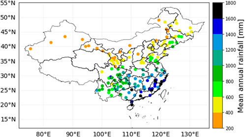
FIGURE 1. Spatial distribution of weather stations in this study. The mean annual precipitation from 2000 to 2019 of each station is given by color.
Grid re-forecasts were extracted based on the locations of the study stations. The re-forecasts of the nearest grid point to a given station were used as the raw ensembles for the EMOS and NN methods. Considering that image-like data are required as the inputs of the convolutional-neural-network (CNN) model, 21 × 21 windows of re-forecasts centered on each of the given stations were extracted. By matching the time periods of the re-forecasts and observations, a total of 7,305 training samples were obtained for the period 2000–2019. As noted above, in the general experiments, we made use of the data from 2018, 2019, and the other 18 years for validation, testing, and training, respectively. To test the influence of the size of the training dataset on the model performance, a sensitivity experiment using two-year data from 2016 to 2017, five-year data from 2013 to 2017, and ten-year data from 2008 to 2017 for training was further performed.
As discussed in Section 1, the CSG EMOS method proposed by Scheuerer and Möller (2015) outperforms the gamma BMA and GEV EMOS for probabilistic precipitation forecasting. Here, we therefore implement the CSG EMOS approach as the baseline. The CSG EMOS model is a variant of the EMOS method based on a CSG distribution specially designed for precipitation. If the shape k > 0 and the scale θ > 0, then the PDF and CDF of a general gamma distribution Γ(k, θ) can be respectively formed as:
and
The shape and scale parameters k and θ can also be replaced by the more commonly used mean μ and standard deviation σ:
Here, we introduce a shifted parameter δ > 0, which transforms the standard gamma distribution to a shifted gamma distribution that is left-censored at zero and whose CDF can be written as:
Considering that the gamma distribution PDF is not analytically integrable, the PDF of a shifted gamma distribution can be formed as:
Note that although the formula is a piecewise function, the PDF of a shifted gamma distribution is continuous for non-negative values of x.
In the CSG EMOS framework, the k and θ parameters of the predictive PDF are usually represented by μ and σ2 using Eq. 3. We suppose an EPS containing m individual ensemble forecasts with notation f1, f2, … , fm for a given station and forecast time. Then, μ and σ2 can be computed by:
where a, (b1, b2, … , bm), c, and d are non-negative regression coefficients. According to Eqs 3, 5, and 6, the predictive PDF of CSG EMOS can be obtained from the raw forecasts of the EPS’s ensemble members and the regression coefficients, which can be estimated from the training data by optimizing an appropriate scoring rule. The IGN and the CRPS are the two most popular scoring rules in the atmospheric sciences for probabilistic forecasting; however, the CRPS has been proven to be more robust (Gneiting et al., 2005; Scheuerer and Möller, 2015), so we use this as the scoring rule here. The CRPS can be written as:
where y is the observation of the targeted variable, F(⋅) is the CDF of the targeted variable with estimated parameters, and H(⋅) is the Heaviside step function, which is 0 if x ≤ y and 1 otherwise. This is expressed in a simplified form following Scheuerer and Möller (2015) in the CSG EMOS:
where CDFk,δ and CDFk,θ,δ are the CDFs of a gamma distribution and a shifted gamma distribution, shown in Eqs 2 and 4, respectively, and B(⋅) is the Beta function. By minimizing the mean CRPS over a rolling training period using maximum-likelihood estimation, the predictive regression coefficients are applied to the ensemble-member forecasts in an independent validation period. The CSG EMOS approach was implemented with the help of the ensembleMOS package in R (Jordan et al., 2017).
Deep NNs show advantages for tackling complex nonlinear tasks with large volumes of data (Hinton and Salakhutdinov, 2006). With the help of layer-wise pre-training, DL-based models mitigate the issue of gradient diffusion and are able to learn features from high-dimensional data. CNN models are typical DL models, and they are the most commonly used models for extracting spatial information. Generally, CNN models comprise an input layer, convolutional layers, pooling layers, fully connected layers, and an output layer. In the convolutional layers, a convolution operation (*) is applied to the grid-like topology input in a given sliding step. This can be read as: s = x*w, where x denotes the input, w is the convolutional kernel or filter, and s refers to the feature map. A pooling function in the pooling layer modifies the feature maps from the previous convolutional layers using a summary statistic, which is usually the maximum and average, to the nearby outputs. The use of convolutional layers and pooling layers is viewed as an efficient approach for the filtering and sharpening of the raw input data.
In our study, both a shallow NN and a deep CNN model were used for the post-processing of probabilistic precipitation forecasting. The two models were implemented as end-to-end architectures, and their workflows are presented in Figure 2. In these models, for a given station, the raw ensembles of re-forecasts (five ensemble members) are used as the inputs. The NN model consists of two hidden layers, which respectively have 16 and 32 neural nodes, with a dropout rate of 0.1. The glorot_uniform scheme (Glorot and Bengio, 2010) is used to initialize the kernels and biases of the neural nodes, and an L2 regularizer is further added to the kernels. The rectified linear unit (ReLU) (Agarap, 2018) is applied as the activation function between the hidden layers, and a linear activation function is used between the last hidden layer and the output layer.
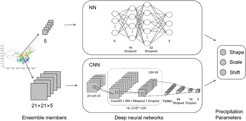
FIGURE 2. Illustration of the workflows using DL-based architectures.
As noted above, a 21 × 21 window of re-forecasts was extracted for a given station as the inputs of the CNN model. The CNN architecture used in our work consists of k convolutional blocks followed by two fully connected layers (see Figure 2). In each convolutional block, there is a 2D convolutional layer with C features followed by a batch-normalization layer (Santurkar et al., 2018), a max-pooling layer, and a dropout layer (Srivastava et al., 2014) with a dropout rate of 0.1. The number of features C is doubled after each convolutional block. The convolutional blocks are repeated twice with k equal to 2, and C0 was set to 16 in our experiments. Within the 2D convolutional layer, a filter size of 3 × 3 is fixed with a slide of 1, and ReLU is used as the activation function.
Both the shallow NN and deep CNN models were used to predict the three precipitation parameters—shape, scale, and shift—following the CSG EMOS approach and the work of Ghazvinian et al. (2021) and Li et al. (2022). These three parameters, as well as the precipitation observations, were further used to calculate the CRPS loss (see Eq. 4) of the DL models. The Adam algorithm (Kingma and Ba, 2014) was used as the optimizer with an initial learning rate of 1 × 10⁻⁴, and the total number of training epochs was fixed as 300. A learning-rate-decay scheduler was integrated to linearly decrease the learning rate from to 1 × 10⁻⁴ to 1 × 10⁻⁵, which starts at the 250th epoch and ends at the 300th epoch. Both the NN and CNN models were implemented with TensorFlow (Abadi et al., 2015) and Keras (Chollet et al., 2015).
To quantitatively evaluate the performance of the post-processed forecasts, the mean CRPS was computed for each station over the testing period. As shown in Eq. 7, the CRPS measures the sum of the squared differences of the cumulative probability space for the probabilistic forecasts in a continuous way. It demonstrates how well the forecasts predict the possibility against the observations. Similar to the root-mean-square error in deterministic forecasting, the CRPS is negative orientated and the perfect value is 0. Additionally, the Brier score (BS) (Williams et al., 2014) was computed to assess the model performance for precipitation events exceeding a given threshold. The BS can be written as:
where y is the observation of the targeted variable, x is the specific threshold, F(⋅) is the CDF of the targeted variable with estimated parameters, and H(⋅) is the Heaviside step function, which is 0 if x ≤ y and 1 otherwise. Looking at Eq. 7, it can be seen that the CRPS is the integral of the BSs at all the possible thresholds. Here, we calculate the BSs with four different thresholds (0, 10, 25, and 50 mm), which respectively represent light precipitation, moderate precipitation, heavy precipitation, and rainstorms for 24-h accumulated precipitation. Calculation of the skill scores of the CRPS and BS is proposed to assess the improvements in the post-processed forecasts compared to the reference forecasts (i.e., the raw re-forecasts). These are defined as:
and
Both of these skill scores are positively oriented. Reliability diagrams were plotted to evaluate the consistency of the raw ensembles and the post-processed forecasts with observations exceeding a given threshold. The diagrams show the binned forecast probability and observed relative frequency of precipitation events exceeding a specific threshold: the more concentrated the data points on the main diagonal, the better the obtained performance. As with BS, 0, 10, 25, and 50 mm were used as the thresholds in the reliability diagrams, and the whole units were divided into 11 bins with values of 0.0, 0.1, 0.2, … , 1.0.
In this section, the overall model performance in terms of the averaged CRPS and BS over the entire 2019 testing period is presented. Reliability diagrams are plotted to show how well the models simulate the probability of predicted precipitation against the observations. The station-by-station model performance is assessed, followed by giving the spatial distribution of the skill scores. The best-performing models in terms of the CRPS and BS at each study station are further exhibited. Finally, two cases using post-processing methods are illustrated to intuitively visualize the model performance.
Figure 3A shows boxplots of the station-wise CRPS with lead times of 1–7 days using the proposed post-processing models. The CRPS values are averaged over the entire 2019 testing period at each study station. All of the post-processing methods remarkably reduce the CRPS with all the lead times, and the CNN model significantly outperforms the other two approaches (EMOS and NN). The interquartile ranges in the boxplots indicate the forecast uncertainty of each model. The plots show that the performance of raw ensembles varies significantly among the study stations. The EMOS and NN models perform competitively in narrowing this disparity, while the CNN approach is even better. With an increasing number of lead days, the improvements of the CNN model compared to the EMOS and NN approaches decrease, but the CNN model is still superior to the others.

FIGURE 3. (A) Boxplots of the mean continuous ranked probability scores (CRPS) of the raw ensemble re-forecasts (ENS) and calibrations using different post-processing methods (EMOS: ensemble model output statistics; NN: shallow NN; and CNN: convolutional NN) for 24-h accumulated precipitation over the entire 2019 testing period with lead times of 1–7 days; (B) as with panel (A), but the CNN models were trained with two-year data (CNN_2y), five-year data (CNN_5y), ten-year data (CNN_10y), and 18-years data (CNN_18y); the red dotted lines are the averaged CRPS values of EMOS for all the study stations over the entire 2019 testing period with lead times of 1–7 days.
To test the impact of the size of the training dataset on the DL-based models, we made use of two-year data from 2016 to 2017, five-year data from 2013 to 2017, ten-year data from 2008 to 2017, and 18-year data from 2000 to 2017 to train the CNN model, and the resulting comparison is given in Figure 3B. This shows that increasing the number of training samples can further improve the performance of the model. However, the improvements are not as significant as we expected, especially when moving from using ten-year data to 18-year data. This indicates that the CNN model is able to capture the statistical dependence between the raw ensembles and the observations in our study using ten-year training samples. Similar results can be seen in the recent work of Gong et al. (2022).
Figure 4 presents the model performance in terms of the BSs of four different thresholds with lead times of 1–7 days. This shows that all the proposed post-processing methods can significantly reduce the BS of the 0-mm threshold with all the lead times, and the CNN model is superior to the others. This indicates that the post-processing methods can distinguish rain or no-rain events well. With an increasing threshold, the improvements brought about by the post-processing methods decrease, but the CNN model is still dominant among them. This demonstrates that the CNN model is practical for calibrating the PDF, even for heavy or extreme precipitation events.

FIGURE 4. As Figure 3, but for the mean Brier scores of different thresholds: (A) 0 mm; (B) 10 mm; (C) 25 mm; and (D) 50 mm.
A comparison between the binned forecasts generated by the raw ensembles and the post-processing methods and the observed relative frequency is given in the reliability diagrams (Figure 5). As with BS, four thresholds were used to evaluate the model performance for different intensities of precipitation with a lead time of 1 day. The raw ensemble (ENS) line, which lies in the bottom-right corner (Figure 5A), indicates that the raw ensembles tend to generate more rainy forecasts than the observations, which results in wet deviations. The more concentrated points generated by the post-processing methods on the main diagonal demonstrate that the proposed models can accurately calibrate probabilistic forecasts and mitigate the wet-deviation issue. However, with an increasing threshold, the EMOS and NN models start to perform unsteadily and fail to maintain high consistency between the binned forecasts and the observed relative frequency. Surprisingly, the CNN model can still provide reliable forecasts for heavy or extreme precipitation events. The concentrated points close to the 1:1 reference line (Figures 5C and D) indicate that the CNN model is able to generate forecasts that share similar probabilities as the observations for precipitation events exceeding 25 and 50 mm.
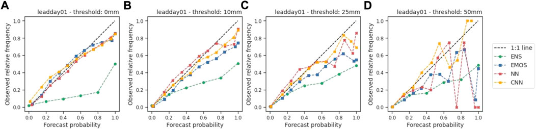
FIGURE 5. Reliability diagrams of the binned raw ensemble re-forecasts (ENS) and the binned calibrations using different post-processing methods (EMOS: ensemble model output statistics; NN: shallow NN; and CNN: convolutional NN) against the observed relative frequencies of 24-h accumulated precipitation over the entire 2019 testing period with a lead time of 1 day with different thresholds: (A) 0 mm; (B) 10 mm; (C) 25 mm; and (D) 50 mm.
To assess the model performance at each study station, the spatial distributions of the skill scores (CRPSS and BSS) are presented in Figures 6 and 7, in which the warm tones indicate positive improvements. This shows that all the proposed post-processing methods can greatly improve the model performance in most of the study stations (see Figure 6). With a lead time of 1 day, EMOS obtains remarkable improvements over Central China and slight improvements in the Beijing–Tianjin–Hebei region, Yangtze River Delta, and Pearl River Delta. Similar results are achieved by using DL-based models, but CNN performs much better in the Yangtze River Delta and the Beijing–Tianjin–Hebei region. It is noted that NN performs invalidly at some stations in Southeast China, since the shallow NN model failed to learn the features of the raw ensembles over the training period, generating “inf” forecasts. With increasing lead times, the improvements of EMOS decrease, and negative performance is even exhibited at some study stations in the Beijing–Tianjin–Hebei region. However, although similar performance degradation is shown, almost all study stations still obtain significantly positive improvements using the CNN model.
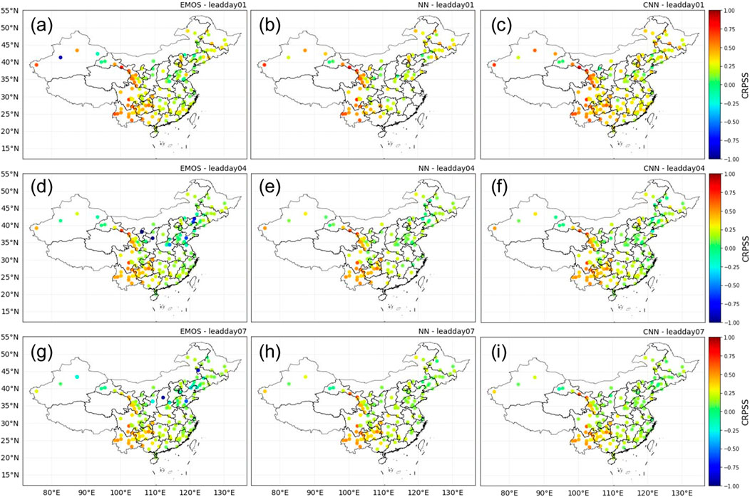
FIGURE 6. Spatial distributions of the continuous ranked probability skill scores (CRPSS) of calibrations using different post-processing methods (EMOS: ensemble model output statistics; NN: shallow NN; and CNN: convolutional NN) with the raw ensembles as the reference forecasts.
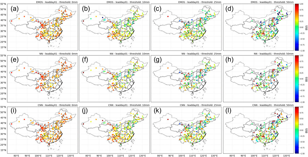
FIGURE 7. Spatial distributions of the Brier scores (BS) of calibrations using different post-processing methods (EMOS: ensemble model output statistics; NN: shallow NN; and CNN: convolutional NN) with the raw ensembles as the reference forecasts. The BSS was computed with a lead time of 1 day for different thresholds: 0, 10, 25, and 50 mm.
Figure 7 presents the spatial distribution of BSs using the proposed post-processing methods for different precipitation thresholds with a lead time of 1 day. This shows that all the post-processing methods can significantly improve the probabilistic forecasts for rain or no-rain events at all the study stations. With increasing thresholds, the EMOS performance degrades, and negative improvements are observed at some stations in North China and the Yangtze River Delta. Similar spatial patterns of the BSs are obtained using CNN, while the improvements at the study stations are significantly higher than those obtained using EMOS.
Maps showing the best-performing models in terms of the CRPS and BS are presented in Figures 8 and 9, respectively. The best-performing model is verified by the best mean scores over the entire 2019 testing period for each study station. As shown in Figure 8, the performance of CNN is dominant for the majority of the stations (74.5%) with a lead time of 1 day, especially for the Yangtze River Delta and Pearl River Delta. With increasing lead time, the performance of NN gradually improves, and in general, the DL-based models perform best at over 75% of study stations with all lead times.
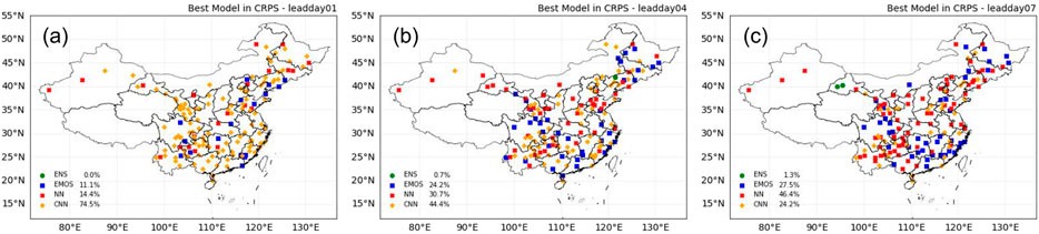
FIGURE 8. Spatial distributions of study stations color coded by the best-performing model (ENS: raw ensembles; EMOS: ensemble model output statistics; NN: the shallow NN; and CNN: convolutional NN) in terms of the continuous ranked probability score (CRPS) with lead times of: (A) 1 day; (B) 4 days; and (C) 7 days. The percentages of the different models performing as the best model are listed in the bottom left.
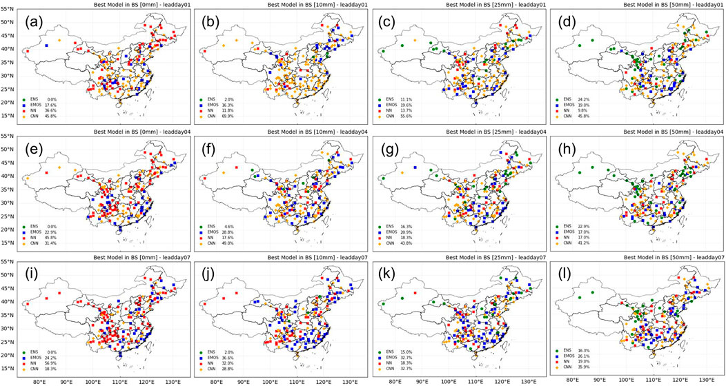
FIGURE 9. Spatial distributions of study stations color coded by the best-performing model (ENS: raw ensembles; EMOS: ensemble model output statistics; NN: the shallow NN; and CNN: convolutional NN) in terms of the Brier skill (BS) for different thresholds with lead times of 1, 4, and 7 days. The percentages of the different models performing as the best model are listed in the bottom left.
Figure 9 presents more details regarding which model performs best for different intensities of precipitation at each study station. This shows that CNN is superior to the other models for all intensities of precipitation with a lead time of 1 day, which is consistent with its performance in terms of the CRPS. However, when the lead time increases, the NN model significantly outperforms the others for the post-processing of light precipitation events. Its remarkable calibration for light precipitation means that the NN model performs best at 46.4% of the study stations in terms of the CRPS with a lead time of 7 days (Figure 8C). However, with increasing precipitation thresholds, CNN again becomes significantly superior to the other models, especially for heavy or extreme precipitation events. This demonstrates that CNN is the best model for the post-processing of probabilistic precipitation forecasting with lead times of 1–7 days and, importantly, it is still practical for heavy precipitation events, where the conventional method EMOS and the shallow NN model fail.
Figure 10 visualizes two cases of the calibrated PDF using the proposed post-processing methods with a lead time of 1 day. The two cases were selected randomly among events in which the observed 24-h accumulated precipitation exceeded 10 mm. This shows that CNN can accurately calibrate probabilistic forecasts with a narrow PDF width and a PDF mode closer to the observation. As shown in Figure 10A, the raw re-forecasts provide an accurate prediction whose ensemble mean is close to the observation. In this case, NN generates the “sharpest” PDF, while the mode of CNN prediction is closer to the observation. The second case is more of a challenge since the raw ensemble mean is far away from the observation; this means that the raw re-forecasts fail to provide accurate information. The EMOS model suffers from this issue and generates a PDF whose mode is close to the ensemble mean rather than to the observation. However, both the NN and CNN models are able to mitigate the problem and provide well-calibrated PDFs with narrow widths. In general, the CNN model is more practical in all situations, while NN is somewhat prone to generating smaller precipitation values in the probabilistic forecasting.

FIGURE 10. Illustration of the predicted PDFs of 24-h accumulated precipitation for (A) national ordinary station No. 53913 on 19 August 2019 and (B) national ordinary station No. 57127 on 09 September 2019 using the proposed post-processing methods (EMOS: ensemble model output statistics; NN: shallow NN; and CNN: convolutional NN) with a lead time of 1 day. The vertical dashed lines indicate the raw ensemble means, and the red squares indicate the observations.
In this work, DL-based models are proposed for probabilistic precipitation post-processing. A shallow NN and a deep CNN, as well as the conventional method EMOS, were applied to 153 selected national ordinary stations across China with lead times of 1–7 days. Our results demonstrate that the DL models, especially the deep CNN, significantly outperform the raw ensembles and the EMOS method. The main advantages of applying DL-based models are their ability to capture the features from raw ensembles and to learn the nonlinear dependence between the ensembles and the observations. Compared with conventional parametric models, DL models are more flexible and do not require pre-definition of specific link functions. It is also easy to embed additional predictors, such as corresponding weather variables and ensembles from multiple EPSs.
As discussed in Section 1, the use of long-term historical data and appropriate loss functions are the two crucial points when using DL-based models in probabilistic precipitation post-processing. In this study, re-forecasts generated by a frozen EPS (GEFS-v12) spanning from 2000 to 2019 were collected as the raw ensembles. The use of re-forecast data helps to mitigate the shortage of training samples. A sensitivity test on the size of training data was performed to present its influence on the DL-based model performance. By increasing the number of training samples from two years of data to 18 years, a remarkable improvement can be seen in terms of the CRPS. It should be noted that the DL-based model is not as competitive as the conventional EMOS model with a small training data set of two years. This indicates that the quantity and quality of training samples are critical to obtain a well-trained DL-based model, which outweighs the model architecture to some extent. To obtain a narrow calibrated PDF for precipitation, in this work, the CRPS was computed as the loss function. However, the original expression of the CRPS is an integral form (Eq. 7), which cannot be directly incorporated into NN models. This is mainly because NN-based models optimize the loss by updating the parameters with gradients. Here, a simplified expression of the CRPS for probabilistic precipitation forecasting is given (Eq. 8) following the CSG EMOS method (Scheuerer and Möller, 2015). A similar strategy was applied by Rasp and Lerch (2018), but they only considered temperature forecasts.
Our results indicate that DL-based models are a promising approach to probabilistic precipitation post-processing. The deep CNN model can greatly reduce the CRPS and BS, especially for heavy or extreme precipitation events, with lead times of 1–7 days; furthermore, it serves as the best-performing model at 74.5% of the study stations for the first lead day. Once the DL models are trained, it is more efficient in producing well-calibrated probabilistic precipitation forecasts, and this significantly saves computing time and resources (see also Rasp and Lerch, 2018).
The re-forecast data used in this study can be downloaded from the the NCEP’s FTP server NCEP’s FTP server. The observation data can be obtained from the China Meteorological Data Service Centre.
The study was conceived by XZ and YJ. YJ and LJ contributed to the model development and maintained the code. YJ wrote the original draft. All authors reviewed and edited the manuscript. XZ supervised the entire project.
The work was jointly funded by the National Key Research and Development Program of China (Grant Nos. 2018YFC1507305, 2018YFC1507200, and 2017YFC1502000).
The authors declare that the research was conducted in the absence of any commercial or financial relationships that could be construed as a potential conflict of interest.
All claims expressed in this article are solely those of the authors and do not necessarily represent those of their affiliated organizations, or those of the publisher, the editors and the reviewers. Any product that may be evaluated in this article, or claim that may be made by its manufacturer, is not guaranteed or endorsed by the publisher.
Abadi, M., Agarwal, A., Barham, P., Brevdo, E., Chen, Z., Citro, C., et al. (2015). TensorFlow: Large-scale machine learning on heterogeneous systems. Software available from tensorflow.org
Agarap, A. F. (2018). Deep learning using rectified linear units (relu). arXiv preprint arXiv:1803.08375.
Baran, S., and Nemoda, D. (2016). Censored and shifted gamma distribution based EMOS model for probabilistic quantitative precipitation forecasting. Environmetrics 27, 280–292. doi:10.1002/env.2391
Bloom, S., Takacs, L., Da Silva, A., and Ledvina, D. (1996). Data assimilation using incremental analysis updates. Mon. Weather Rev. 124, 1256–1271. doi:10.1175/1520-0493(1996)124<1256:dauiau>2.0.co;2
Cheng, L., Zang, H., Ding, T., Sun, R., Wang, M., Wei, Z., et al. (2018). Ensemble recurrent neural network based probabilistic wind speed forecasting approach. Energies 11, 1958. doi:10.3390/en11081958
Cho, D., Yoo, C., Im, J., and Cha, D.-H. (2020). Comparative assessment of various machine learning-based bias correction methods for numerical weather prediction model forecasts of extreme air temperatures in urban areas. Earth Space Sci. 7, e2019EA000740. doi:10.1029/2019ea000740
Chollet, F., Ganger, M., Duryea, E., and Hu, W. (2015). Keras. Available at: https://github.com/fchollet/keras.
Düben, P., Modigliani, U., Geer, A., Siemen, S., Pappenberger, F., Bauer, P., et al. (2021). Machine learning at ECMWF: A roadmap for the next 10 years. Eur. Centre Medium-Range Weather Forecasts, Tech. Rep 878.
Fritsch, J., Houze, R., Adler, R., Bluestein, H., Bosart, L., Brown, J., et al. (1998). Quantitative precipitation forecasting: Report of the eighth prospectus development team, us weather research program. Bull. Am. Meteorological Soc. 79, 285–299.
Ghazvinian, M., Zhang, Y., Seo, D.-J., He, M., and Fernando, N. (2021). A novel hybrid artificial neural network-parametric scheme for postprocessing medium-range precipitation forecasts. Adv. Water Resour. 151, 103907. doi:10.1016/j.advwatres.2021.103907
Glorot, X., and Bengio, Y. (2010). “Understanding the difficulty of training deep feedforward neural networks,” in Proceedings of the thirteenth international conference on artificial intelligence and statistics (Sardinia, Italy: JMLR Workshop and Conference Proceedings), 249–256.
Gneiting, T., and Raftery, A. E. (2007). Strictly proper scoring rules, prediction, and estimation. J. Am. Stat. Assoc. 102, 359–378. doi:10.1198/016214506000001437
Gneiting, T., Raftery, A. E., Westveld, A. H., and Goldman, T. (2005). Calibrated probabilistic forecasting using ensemble model output statistics and minimum CRPS estimation. Mon. Weather Rev. 133, 1098–1118. doi:10.1175/mwr2904.1
Gong, B., Langguth, M., Ji, Y., Mozaffari, A., Stadtler, S., Mache, K., et al. (2022). Temperature forecasting by deep learning methods. Geosci. Model Dev. Discuss., 1–35.
Gourley, J. J., and Vieux, B. E. (2005). A method for evaluating the accuracy of quantitative precipitation estimates from a hydrologic modeling perspective. J. Hydrometeorol. 6, 115–133. doi:10.1175/jhm408.1
Guan, H., Zhu, Y., Sinsky, E., Fu, B., Li, W., Zhou, X., et al. (2022). GEFSv12 reforecast dataset for supporting subseasonal and hydrometeorological applications. Mon. Weather Rev. 150, 647–665. doi:10.1175/mwr-d-21-0245.1
Hamill, T. M., Bates, G. T., Whitaker, J. S., Murray, D. R., Fiorino, M., Galarneau, T. J., et al. (2013). NOAA’s second-generation global medium-range ensemble reforecast dataset. Bull. Am. Meteorological Soc. 94, 1553–1565. doi:10.1175/bams-d-12-00014.1
Han, L., Chen, M., Chen, K., Chen, H., Zhang, Y., Lu, B., et al. (2021). A deep learning method for bias correction of ECMWF 24–240 h forecasts. Adv. Atmos. Sci. 38, 1444–1459. doi:10.1007/s00376-021-0215-y
Han, Y., Zhang, G. J., Huang, X., and Wang, Y. (2020). A moist physics parameterization based on deep learning. J. Adv. Model. Earth Syst. 12, e2020MS002076. doi:10.1029/2020ms002076
Harris, L. M., and Lin, S.-J. (2013). A two-way nested global-regional dynamical core on the cubed-sphere grid. Mon. Weather Rev. 141, 283–306. doi:10.1175/mwr-d-11-00201.1
Hatfield, S., Chantry, M., Dueben, P., Lopez, P., Geer, A., and Palmer, T. (2021). Building tangent-linear and adjoint models for data assimilation with neural networks. J. Adv. Model. Earth Syst. 13, e2021MS002521. doi:10.1029/2021ms002521
Hersbach, H. (2000). Decomposition of the continuous ranked probability score for ensemble prediction systems. Weather Forecast. 15, 559–570. doi:10.1175/1520-0434(2000)015<0559:dotcrp>2.0.co;2
Hinton, G. E., and Salakhutdinov, R. R. (2006). Reducing the dimensionality of data with neural networks. science 313, 504–507. doi:10.1126/science.1127647
Ji, L., Zhi, X., Zhu, S., and Fraedrich, K. (2019). Probabilistic precipitation forecasting over East Asia using Bayesian model averaging. Weather Forecast. 34, 377–392. doi:10.1175/waf-d-18-0093.1
Jordan, A., Krüger, F., and Lerch, S. (2017). Evaluating probabilistic forecasts with scoring rules. arXiv preprint arXiv:1709.04743.
Kingma, D. P., and Ba, J. (2014). Adam: A method for stochastic optimization. arXiv preprint arXiv:1412.6980
Li, W., Pan, B., Xia, J., and Duan, Q. (2022). Convolutional neural network-based statistical post-processing of ensemble precipitation forecasts. J. Hydrology 605, 127301. doi:10.1016/j.jhydrol.2021.127301
Majumdar, S. J., and Torn, R. D. (2014). Probabilistic verification of global and mesoscale ensemble forecasts of tropical cyclogenesis. Weather Forecast. 29, 1181–1198. doi:10.1175/waf-d-14-00028.1
McGovern, A., Elmore, K. L., Gagne, D. J., Haupt, S. E., Karstens, C. D., Lagerquist, R., et al. (2017). Using artificial intelligence to improve real-time decision-making for high-impact weather. Bull. Am. Meteorological Soc. 98, 2073–2090. doi:10.1175/bams-d-16-0123.1
Peng, T., Zhi, X., Ji, Y., Ji, L., and Tian, Y. (2020). Prediction skill of extended range 2-m maximum air temperature probabilistic forecasts using machine learning post-processing methods. Atmosphere 11, 823. doi:10.3390/atmos11080823
Raftery, A. E., Gneiting, T., Balabdaoui, F., and Polakowski, M. (2005). Using Bayesian model averaging to calibrate forecast ensembles. Mon. weather Rev. 133, 1155–1174. doi:10.1175/mwr2906.1
Rasp, S., and Lerch, S. (2018). Neural networks for postprocessing ensemble weather forecasts. Mon. Weather Rev. 146, 3885–3900. doi:10.1175/mwr-d-18-0187.1
Ravuri, S., Lenc, K., Willson, M., Kangin, D., Lam, R., Mirowski, P., et al. (2021). Skillful precipitation nowcasting using deep generative models of radar. arXiv preprint arXiv:2104.00954.
Reichstein, M., Camps-Valls, G., Stevens, B., Jung, M., Denzler, J., Carvalhais, N., et al. (2019). Deep learning and process understanding for data-driven Earth system science. Nature 566, 195–204. doi:10.1038/s41586-019-0912-1
Santurkar, S., Tsipras, D., Ilyas, A., and Madry, A. (2018). How does batch normalization help optimization? Adv. neural Inf. Process. Syst. 31.
Scheuerer, M., and Möller, D. (2015). Probabilistic wind speed forecasting on a grid based on ensemble model output statistics. Ann. Appl. Stat. 9, 1328–1349. doi:10.1214/15-aoas843
Scheuerer, M., Gregory, S., Hamill, T. M., and Shafer, P. E. (2017). Probabilistic precipitation-type forecasting based on GEFS ensemble forecasts of vertical temperature profiles. Mon. Weather Rev. 145, 1401–1412. doi:10.1175/mwr-d-16-0321.1
Schultz, M. G., Betancourt, C., Gong, B., Kleinert, F., Langguth, M., Leufen, L. H., et al. (2021). Can deep learning beat numerical weather prediction? Phil. Trans. R. Soc. A 379, 20200097. doi:10.1098/rsta.2020.0097
Sha, Y., Gagne, D. J., West, G., and Stull, R. (2020). Deep-learning-based gridded downscaling of surface meteorological variables in complex terrain. part i: Daily maximum and minimum 2-m temperature. J. Appl. Meteorology Climatol. 59, 2057–2073. doi:10.1175/jamc-d-20-0057.1
Srivastava, N., Hinton, G., Krizhevsky, A., Sutskever, I., and Salakhutdinov, R. (2014). Dropout: A simple way to prevent neural networks from overfitting. J. Mach. Learn. Res. 15, 1929–1958.
Surcel, M., Zawadzki, I., Yau, M., Xue, M., and Kong, F. (2017). More on the scale dependence of the predictability of precipitation patterns: Extension to the 2009–13 caps spring experiment ensemble forecasts. Mon. Weather Rev. 145, 3625–3646. doi:10.1175/mwr-d-16-0362.1
Taillardat, M., Mestre, O., Zamo, M., and Naveau, P. (2016). Calibrated ensemble forecasts using quantile regression forests and ensemble model output statistics. Mon. Weather Rev. 144, 2375–2393. doi:10.1175/mwr-d-15-0260.1
Tallapragada, V. (2019). “Recent updates to NCEP global modeling systems: Implementation of FV3 based global forecast system (GFS v15. 1) and plans for implementation of global ensemble forecast system (EGFSv12),” in AGU fall meeting abstracts, 2019, 34.
Williams, R., Ferro, C., and Kwasniok, F. (2014). A comparison of ensemble post-processing methods for extreme events. Q. J. R. Meteorol. Soc. 140, 1112–1120. doi:10.1002/qj.2198
Zhang, L., Sielmann, F., Fraedrich, K., Zhu, X., and Zhi, X. (2015). Variability of winter extreme precipitation in Southeast China: Contributions of SST anomalies. Clim. Dyn. 45, 2557–2570. doi:10.1007/s00382-015-2492-6
Keywords: deep learning, probabilistic precipitation forecasting, post-processing, loss function, ensemble model output statistics
Citation: Ji Y, Zhi X, Ji L, Zhang Y, Hao C and Peng T (2022) Deep-learning-based post-processing for probabilistic precipitation forecasting. Front. Earth Sci. 10:978041. doi: 10.3389/feart.2022.978041
Received: 25 June 2022; Accepted: 18 August 2022;
Published: 20 September 2022.
Edited by:
Jingyu Wang, Nanyang Technological University, SingaporeReviewed by:
Rui A. P. Perdigão, Meteoceanics Institute for Complex System Science, AustriaCopyright © 2022 Ji, Zhi, Ji, Zhang, Hao and Peng. This is an open-access article distributed under the terms of the Creative Commons Attribution License (CC BY). The use, distribution or reproduction in other forums is permitted, provided the original author(s) and the copyright owner(s) are credited and that the original publication in this journal is cited, in accordance with accepted academic practice. No use, distribution or reproduction is permitted which does not comply with these terms.
*Correspondence: Xiefei Zhi, emhpQG51aXN0LmVkdS5jbg==
Disclaimer: All claims expressed in this article are solely those of the authors and do not necessarily represent those of their affiliated organizations, or those of the publisher, the editors and the reviewers. Any product that may be evaluated in this article or claim that may be made by its manufacturer is not guaranteed or endorsed by the publisher.
Research integrity at Frontiers
Learn more about the work of our research integrity team to safeguard the quality of each article we publish.