Feasibility analysis of early warning of sea fog within six hours for two harbors in the South China Sea

Sea fog significantly impacts harbor operations, at times even causing navigation to cease. This study examines two harbors in the north of the South China Sea, analyzing the feasibility of increasing each harbor’s sea fog early warning capability to 6 h in advance. Although the harbors are separated by only about 100 km, analysis of their backward trajectories reveals differences in the incoming flow and sea fog types. Concerning the types, at Xuwen harbor, warm advection fog represents 49.56% of the cases, cold advection representing 48.03%. At Zhanjiang harbor, 37.06% are warm advection fog, with 58.33% cold advection fog cases. We propose different monitoring and early warning schemes for the harbors. For Xuwen, we suggest eight visibility lidars located on the north and south sides of Qiongzhou Strait (two on the north, six on the south). Here, such a setup would give warning probabilities of sea fog of 87.50, 66.23, and 49.78% for advance times of 2, 3, and 4 h. For Zhanjiang, we suggest two visibility lidars and four buoys at the east side of the harbor. The corresponding warning probabilities are 83.77, 64.47, and 47.15% for the same advance times. For 5–6 h in advance, the early warning probabilities of both harbors drop quickly. We also suggest a flow chart for the early warning and monitoring scheme at each harbor.

1 Introduction

Sea fog has various impacts on human activities, especially for harbor transportation. The fog makes marine transport, coastal traffic, as well as harbor operations much less safe (Wang, 1985; Leipper, 1994; Lewis et al., 2004; Gultepe et al., 2007; Zhang et al., 2009; Koračin et al., 2014; Koračin and Dorman, 2017; Dorman et al., 2019). According to Tremant (1987), 32% of all accidents at sea worldwide occur under a dense fog. Gultepe et al. (2007) pointed out that economic and human losses associated with fog and low visibilities are comparable to the losses from other weather disasters such as tornadoes and typhoons. For example, in China, there were 19 collision accidents caused by poor visibility in 2018, resulting in 30 missing and presumed dead (Maritime Safety Administration of the Ministry of transport of China, 2019).

Sea-fog forecasting remains full of challenges (Lewis et al., 2004; Gultepe et al., 2007; Koračin and Dorman, 2017). Mesoscale numerical modelling has been the primary method of such forecasting ever since Ballard et al. (1991) used a 3-dimensional mesoscale numerical model to forecast the sea fog of Northeast Scotland. Since then, many studies have aimed to improve the ability of sea-fog numerical simulation and prediction for various locations. Such studies include that for the US west coast (Koračin et al., 2001, 2005), the Yellow Sea and the East China Sea (Fu et al., 2006; Gao et al., 2007; Heo and Ha, 2010; Kim and Yum, 2012; Wang et al., 2014; Yang et al., 2019), the South China Sea (Yuan and Huang, 2011; Huang et al., 2016), and the sea fog off the east coast of Canada (Yang et al., 2010; Chen et al., 2020a). Concerning the ability of a long-term operational sea fog model, the model of Huang et al. (2019), with a horizontal resolution of 3 km, gave a 2-years-average equitable threat score (ETS) of 0.20 for 24 h forecasts in the South China Sea. Zhou and Du (2010) used a 10-member multimodel ensemble method, with a horizontal resolution is 15 km, and argued that the ETS score can be improved up to 0.334 for 12- and 36-h forecasts in eastern China and coastal areas.

The South China Sea (SCS) is one of the seven marginal seas with significant sea fog (Dorman et al., 2019). The coast region near Xuwen harbor and Zhanjiang harbor (Figure 1A) has the highest frequency of sea fog in the north part of the SCS (Wang, 1985; Huang et al., 2011, 2015; Zhang and Lewis, 2017; Han et al., 2022). Here, the fog season is usually from January to April. We focus on these two important harbors. Zhanjiang is a deep-water port designed and built by China. It has become one of the 25 major ports along the coast of China and, except for all the fog, has the best navigation conditions in the coastal areas of South China. Xuwen is an important transport port connecting Hainan Province and the Chinese mainland for passenger and freight transport.

FIGURE 1

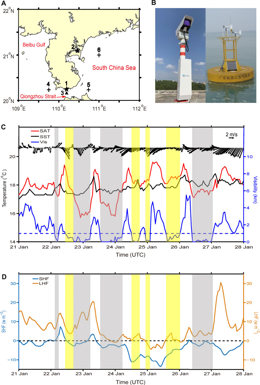
FIGURE 1. Overview of stations, instruments, and data. (A) Locations of 1) Xuwen harbor, 2) Zhanjiang harbor, 3) buoy, 4)—5) Selected points to calculate the average heat flux data for Xuwen. 6) Selected point to represent the heat flux data for Zhanjiang. (B) Monitoring instruments. Left: visibility lidar. Right: buoy. Photo courtesy of Xinxin Zhang. (C) Wind vector, surface air temperature (SAT), sea surface temperature (SST), and visibility at Xuwen harbor for the 202101 fog event. The wind vector, SAT and SST from 3 m buoy data and the visibility from Xuwen station. Yellow bands indicate warm advection fog, gray bands indicate cold. The adjacent yellow–gray band at 23 January is classified as abnormal “A” in Table 3. (D) Sensible heat flux (SHF) and latent heat flux (LHF) at Xuwen based on ERA5 data.

Advection fog is the dominant type in SCS (Wang 1985). In general, two kinds of advection fog can occur over sea. One is warm advection fog in which the surface air temperature (SAT) exceeds the sea surface temperature (SST), the other is cold advection fog with SAT below SST (Taylor, 1917; Petterssen, 1938; Pilié et al., 1979; Findlater et al., 1989; Tachibana et al., 2008; Tanimoto et al., 2009; Huang et al., 2015). The warm advection fog and cold advection fog are the same as cold sea fog and warm sea fog in Koračin et al. (2014). Based on 60 fog cases observed at the Marine Meteorological Science Experiment Base (MMSEB) at Bohe, Maoming in 2007–12, Huang et al. (2015) found about 69% to be warm advection fog, 28% cold advection fog, and 3% being other types. The MMSEB is about 100 km from Zhanjiang harbor and about 180 km from Xuwen harbor, with different geographical and climatic characteristics (Compilation group of Guangdong Provincial Meteorological Bureau, 2006). Because different types of advection fog correspond to different synoptic situations, and the synoptic situation is a key factor to be considered in sea fog early warning, one goal of this study is to determine percentages of each fog type at the two harbors.

Both Xuwen and Zhanjiang harbors are seriously affected by sea fog weather during the fog season. For example, constant sea fog occurred from 15 to 25 February 2018 in Zhanjiang, with the minimum visibility less than 200 m, causing the suspension of shipping in Qiongzhou Strait. In this period, two ships collided here, resulting in two fatalities. Furthering the disruption, this period included China’s spring Festival holiday with all of its increased travel and transport demand. For example, it resulted in a large number of passengers stranded. The queue for ferry service was as long as 20 km at the peak, with some people waiting in their car over day. Given such a major disruption, the Maritime Safety Administration later argued for an accurate early warning of sea fog within 6 h to help them to adjust the ferry operations. This urgent demand prompted this study.

What is the best method to predict sea fog within 6 h? Kamangir et al. (2021) predicted fog visibility for an airport by post-processing numerical weather prediction model output and satellite-based sea surface temperature using a 3D-Convolutional Neural Network (3D-CNN). Although they could give 6 h sea-fog forecast results, this method is based on model output, which is limited by the initial field preparation time and the running time of the model. Thus, it may be difficult to release the method’s results 6 h ahead of the fog event. The most effective means for early warning of sea fog is by making direct observations. For example, Xian et al. (2020) suggest using visibility lidar systems.

Since 2019, Hainan Meteorological Bureau has built three visibility lidars to monitor the harbors and channels on both sides of the Qiongzhou Strait. The complementary observation of the lidar, together with satellite cloud images, works well to not only monitor the fog, but also improve the early warning ability (Chen et al., 2020b). However, for early warning of a harbor, further improvements are needed. For example, visibility lidar has a scanning radius of only 15 km. For advection fog, the early warning time is about 1–2 h (for a windspeed of 3 m s⁻¹). Also, satellites do a poor job distinguishing fog from low cloud (Bendix, 1995; Lee et al., 1997; Bendix et al., 2006; Zhang and Yi, 2013; Wilcox, 2017). The retrieval ability of satellite between sea fog and low cloud is particularly poor for warm advection fog as the two types often occur together (Huang et al., 2011, Huang et al., 2015). Hence, in addition to satellite monitoring, direct monitoring may be critical for early warning of sea fog. A feasibility analysis of early warning of sea fog would help determine the best method to reach the goal of a 6-h warning system.

This study focuses on the feasibility of advancing the early warning time of sea fog in Xuwen and Zhanjiang harbors to 6 h, and how to effectively arrange the monitoring instruments and equipment. The present paper is organized as follows: Section 2 describes the data and method used in this study. Section 3 analyses the backward trajectory frequency and the proportion of both types of advection fog for the harbors. Section 4 analyses the feasibility of sea fog early warning and provides early warning and monitoring schemes. Section 5 presents the main conclusions and discussion.

2 Data and method

2.1 Data

We use five sources of data: observations of meteorological stations, buoy data, climatological sea surface temperature (SST), analyzed products on gridpoints and heat flux data. The observations are operated by the China Meteorological Administration (CMA) and are from a weather station at Xuwen (110.16 ^oE, 20.24^oN) and one at Zhanjiang (110.40^oE, 21.20^oN) (Figure 1). These two stations are within 3 km of their harbor. The stations provide data at intervals of 5 minutes, including wind direction, windspeed, temperature, air pressure, dew point temperature, precipitation, relative humidity, visibility, radiation, soil temperature, and cloud cover. In 2021, a buoy of diameter 3 m was placed in the middle of Qiongzhou Strait, mainly for sea fog monitoring. The main meteorological elements observed from buoy include wind direction, windspeed, temperature, humidity, air pressure, and sea surface temperature (Figure 1).

As the harbors are separated by only 100 km, fog generally occurs at both at the same time, especially for a continuous sea fog event. A fog event is defined as occurring when the visibility is less than 1 km at both stations with some port activities being suspended for three or more days. For 2013–2021 there were 13 such events with the total port-suspension duration of 57 days. In all events, the port suspension occurred at both harbors on the same days (Table 1).

TABLE 1

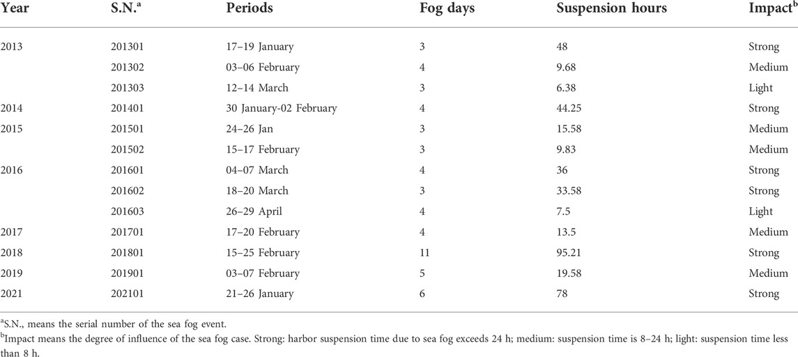
TABLE 1. The 13 sea fog events at both harbors in 2013–2021.

The climatological SST data comes from the National Oceanic and Atmospheric Administration daily optimum interpolation sea surface temperature (DOISST) Version 2.1 (Huang et al., 2021). This dataset covers from September 1981 to December 2021 and is on a 1/4 degree global grid. The gridded, analyzed data is from the Global Forecast System (GFS), which is a global numerical weather prediction system containing a global computer model and variational analysis run by the U.S. National Weather Service (NWS). The GFS is run four times a day, and produces forecasts for up to 16 days in advance. The forecast component uses the FV3 (finite volume cubed) model with a resolution of ∼13 km. The analyzed data is an archive of concatenated short-term GFS forecast model output having a 1/4 degree latitude–longitude grid on 55 hybrid levels. The data is hourly forecast data and can be downloaded at https://www.ready.noaa.gov/archives.php. Details about GFS are at https://www.emc.ncep.noaa.gov/emc/pages/numerical_forecast_systems/gfs.php.

We use the hourly surface sensible heat flux and surface latent heat flux from the European Centre for Medium-Range Weather Forecasts (ECMWF)’s ERA5 dataset. This dataset is the fifth generation ECMWF reanalysis of global climate and weather for the past 4–7 decades (currently, data is available from 1959). ERA5 combines model data with observations and has a horizontal resolution of 0.25 degree. (Reanalysis does not have the constraint of issuing timely forecasts and accommodates improved versions of the original observations to improve the quality of the product (Hersbach et al., 2020). The download web site is https://cds.climate.copernicus.eu/cdsapp#!/dataset/reanalysis-era5-single-levels?tab=form.)

To evaluate the ERA5 heat fluxes, we selected a sea fog event in 2021 (the 202101 fog event), and compare it with the buoy data. Except for the cases of sea fog on January 22–23, the winds are mainly northeast and east (Figure 1C). Figure 1C also shows the changes of buoy SAT and SST data, indicating that this sea fog event includes both the cold advection fog (SAT ≤ SST) and the warm advection fog (SAT > SST). The overall trend starts from mainly cold advection fog, goes to warm advection fog, and then changes back to cold advection fog again. As pointed out in Huang et al. (2015), the direction of the heat flux of the cold advection fog is generally upward (from sea to air), whereas that of the warm advection fog is the opposite. The ERA5 data in Figure 1D show trends in sensible heat flux and latent heat flux that are consistent with the trends in buoy data. Given the 0.25 degree resolution of the ERA5 data, we use the average value of two over sea points on both sides of Xuwen harbor to represent the value of Xuwen harbor to reduce the influence of land on the over sea data. Similarly, we use the value of over sea on the east side of Zhanjiang harbor to represent the value of Zhanjiang harbor (Figure 1A).

2.2 Method

We use the NOAA hybrid single-particle Lagrangian integrated trajectory (HYSPLIT) model to calculate the backward tracking trajectory of the air mass and find the source of sea fog (Draxler and Hess 1998). This model was originally developed to calculate and analyze the transport and diffusion trajectory of air pollutants. It is often used to determine the origin of air masses and establish source–receptor relationships (Fleming et al., 2012). With continual improvement over 30 years (now latest version is HYSPLIT 5), it has been widely applied in the atmospheric sciences to track the source of air particles backward, determine the source of an air mass, and to help establish a relationship between the source and the affected place (Stein et al., 2015).

To analyze the source of sea fog, we run off-line HYSPLIT backwards for 72 h at the harbor location at six levels (10, 100, 300, 500, 800, and 1,500 m above sealevel). On a given sea-fog day, we ran the model every 3 h, making a total of 456 runs for each harbor. Similar to Dorman et al. (2019), we interpolate the backward trajectory data to a 0.05 degree grid over land and sea. Then we calculate the backward-trajectory frequency of each gridpoint, meaning the fraction (or number) of trajectories that passed over that point for the previous hours (for example, 1, 6, or 72 h). The early warning probability per hour is computed by the sum of gridpoints that can be detected with the sea fog monitoring instruments divided by the total runs (456) when fog approaches. Here, we define each run as one sea fog case. Hence, there are many sea fog cases in every fog event.

We consider here two instruments for monitoring and providing an early warning of sea fog: visibility lidar and offshore buoys. Examples are shown in Figure 1B. At present, the maximum range of visibility lidar is 15 km, though the actual effective detection range may be less. The buoy’s effective observation range is 10 km if it has video monitoring equipment.

The initial cost of an over-sea buoy is about 3–5 times that of the visibility lidar, and due to its location, is difficult to operate and maintain. In comparison, although the monitoring effect of a visibility lidar may be better than that of a buoy, it is usually installed on shore because it requires a long-term stable power supply to achieve effective continuous monitoring.

Although we define warm advection fog and cold advection fog according to the air-sea temperature difference, we do not have buoy observation data for all sea fog events from 2013 to 2021. Also, we found that the air–sea temperature difference from the reanalysis data (such as ERA5 data) was not consistent with the actual observation value for 202101 sea fog event. Hence, we cannot distinguish warm advection fog and cold advection fog directly by the air–sea temperature difference, but through an indirect method, that is, by analyzing the backward trajectory of the air flow at a low altitude of 10 m, and checking the result against the heat flux from the ERA5 data. See Section 3.2 for more details.

3 Backward trajectory frequency and advection fog types

3.1 Features of the backward trajectory frequency

The occurrence and development of sea fog is very sensitive to SST. Here we calculate a 40-years (1982–2021) climatological mean of SST during the main fog season from January to March for the northern SCS and surrounding areas. Because of the East Asian monsoon (Tao and Chen, 1987), the prevailing surface wind during the fog season is from the northeast, cooling the sea surface off the southern China coast. The resulting cold water along the coast contributes to the formation of sea fog (Wang, 1985; Huang et al., 2015; Figure 2).

FIGURE 2

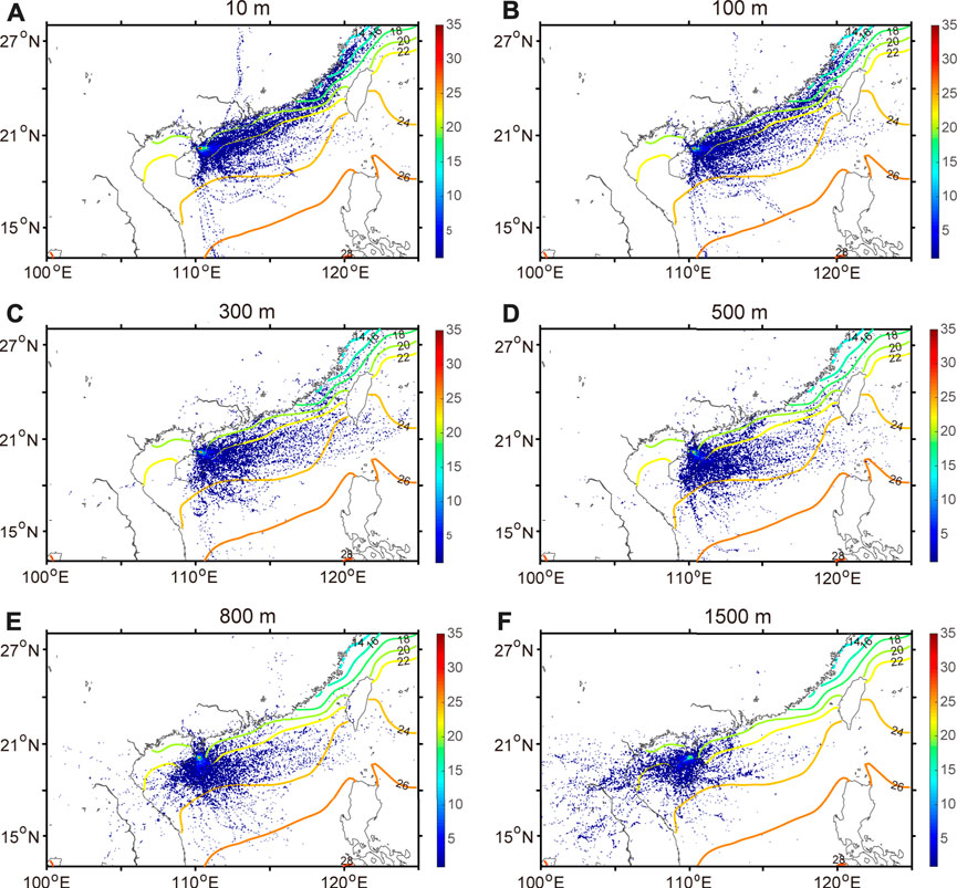
FIGURE 2. Number of 72 h backward trajectories for each level at Xuwen harbor during all sea fog events in 2013–2021. (A–F) represents 10, 100, 300, 500, 800, and 1500 m of the trajectory above sea level. Scale is number passing over a given gridpoint out of the 456 runs. Contours show the climatological mean of January–March SST for 1982–2021 (°C).

For all sea fog cases in 2013–2021, the 72-h backward trajectories from Xuwen at each level show different features. At the 10 m level (Figure 2A), the main direction of the backward trajectory is northeast along the coast. Along this direction, the gridpoint with the largest number has the value 48. East and south trajectories are also common. With the height rising from 100 to 500 m, the primary direction of the backward track flow changes from northeast to east (Figures 2B–D). At 800 m, although the easterly flow is still primary, the southerly and westerly flows become more common (Figure 2E). At 1,500 m, the main flow from the backward trajectory has turned to the west (Figure 2F). In general, with the height changing from low to high, the inflow direction changes clockwise from northeast to west.

The analogous backward trajectories from Zhanjiang harbor are similar to those from Xuwen (Figure 3). However, at the 10 and 100 m levels, the main backward trajectory flow direction is more northerly than that from Xuwen and closer to the coastline (Figures 3A,B). At the 10 m level, the maximum number is approximately 35, smaller than that of Xuwen, a relation that holds at all levels, suggesting that the source direction of sea fog is more complex and elusive (Figures 3C–F).

FIGURE 3

FIGURE 3. Same as Figure 2, but for Zhanjiang harbor.

To make a more detailed comparison between Xuwen and Zhanjiang harbor, we calculated the frequency difference between their backward trajectories. Results in Figure 4 show that at the 10 and 100 m levels, Zhanjiang harbor has more trajectories from the north (N), northeast (NE), and east–northeast (ENE). Conversely, Xuwen harbor has more incoming flow from the east (E), southeast (SE) and south (S). At the 300 and 500 m levels, both harbors show incoming flow from the SE and S. At 800 m, the flow is more southwest and west. Similarly, both harbors have more from the west at the 1,500 m level. The largest difference in the incoming flow is in the lower layer. The difference in the lower layer determines the difference in the underlying sea surface through which the air flows, which may affect the sea fog formation.

FIGURE 4

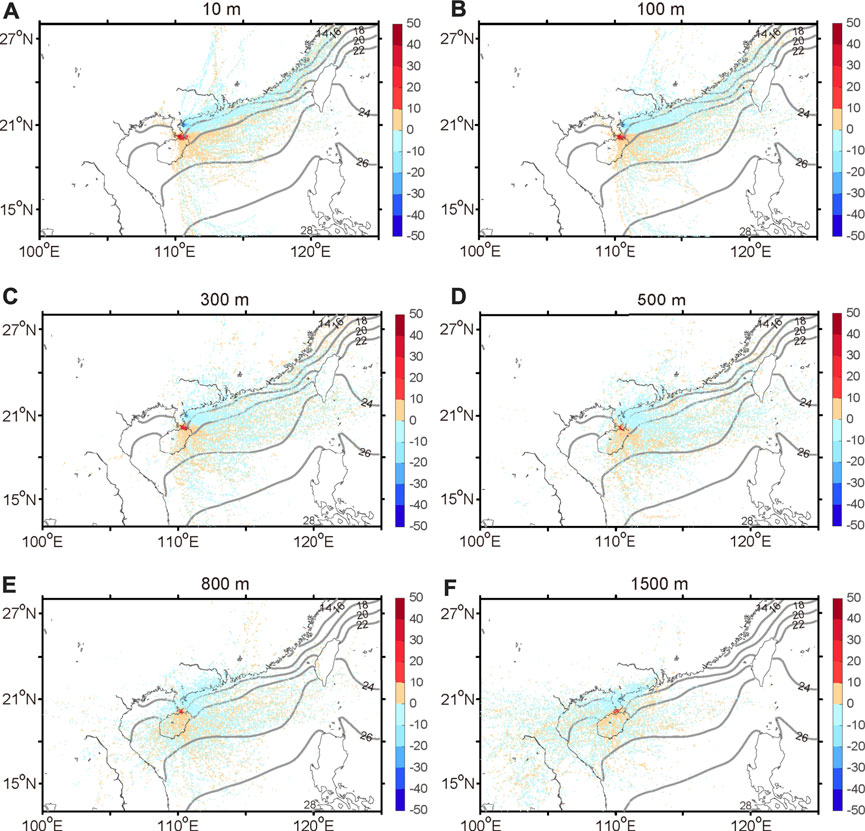
FIGURE 4. Difference in frequency of backward trajectories between Xuwen and Zhanjiang harbors. (A–F) represents 10, 100, 300, 500, 800 and 1500 m of the trajectory above sea level. Contours are the same as in Figure 2.

3.2 Proportion of advection fog types

In general, the cold advection fog type occurs when the low-level flow comes from a colder SST area (Huang et al., 2015). For these harbors, this direction is NE, ENE, and E. Conversely, the low-level flow for warm advection fog mainly comes from a warmer SST area. However, a change between the cold and the warm advection fog types can occur during a single sea fog event in the North SCS.

For such changes between the two fog types, we recognize that two main types can occur. One type is that which occurs in the same sea fog process. For example, when a warm type fog forms, but then the air cools due to fog-top longwave cooling from the fog top, producing a cold type fog (Findlater et al., 1989; Yang et al., 2018). However, we did not have sufficient data to check for this possibility and instead relied upon the second type of change below.

This second type involves a change of near surface incoming flow caused by a change in the synoptic situation. For example, it can be seen in Figure 1C that the occurrence of an abnormal northwest wind is the reason that the cold advection fog changed from a warm type during January 22–23. Furthermore, compared with the cold advection fog on January 24, the warm advection fog on January 25–26 has little difference in the wind near the ground (Figure 1C). Therefore, it is necessary to distinguish whether warm advection fog or cold advection fog should occur based on the near surface backward incoming flow.

Here, we use a method similar to that in Huang et al. (2015) to distinguish cold-from warm-advection fog over the sea. In this method, the direction of the lowest backward trajectory is critical: if the 10 m flow comes from a cold SST area on the coast (e.g., NE, ENE, or E directions), we assume it will form cold advection fog. Otherwise, if the 10 m flow comes from the warm SST area (e.g., E, SE, and S directions), we assume it will form warm advection fog. There remain some complex paths that are hard to categorize that we label as abnormal paths (Figure 5). In addition, we use the ERA5 heat flux data to help distinguish the cold from the warm advection fog according to the direction of heat flux (i.e., upward indicating the cold type). After using the two methods at both harbors, we found that about 70% of the sea fog cases have consistent evolution characteristics as described by the two methods. When there are inconsistencies, we take the 10 m flow method as the standard.

FIGURE 5

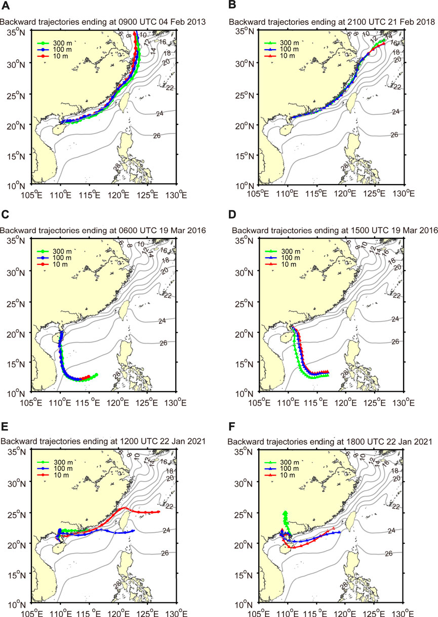
FIGURE 5. Trajectories for the fog types. Left side: Xuwen harbor. Right side: Zhanjiang harbor. Top row (A,B): Typical trajectory for cold advection fog. Middle row (C,D): warm advection fog. Bottom row (E,F): abnormal paths.

The case with easterly flow to Xuwen harbor sometimes is difficult to judge by the 10 m flow method. In this direction, although the nearby sea is relatively cool, distant sea has a warm SST (Figure 5). In this case, we argue that warm advection fog occurs when the easterly incoming flow exceeds 400 km (i.e., about 37 h for a 3 m s⁻¹ windspeed). In such a case, sufficient heat- and water-vapor exchange between the sea and the air has occurred. Otherwise, we consider that cold advection fog forms.

Applying the above methods to the 456 backward trajectory runs, we find for Xuwen 49.56% warm advection fog cases and 48.03% cold advection fog cases. For Zhanjiang, the results are 37.06% warm advection fog cases and 58.33% cold advection fog cases (Table 2). Hence, Xuwen harbor has 12.5% more warm advection fog cases and 10.3% fewer cold advection fog cases than that in Zhanjiang harbor. The result arises from the difference of backward trajectories for the two harbors; specifically, the Xuwen harbor has more southeast and southward incoming flows in the low level, resulting more warm advection fog cases (Figure 4A).

TABLE 2

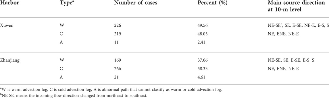
TABLE 2. Main characteristics of advection fog cases for 2013–2021.

In our analysis of the backward trajectories of these sea fog cases, we also find that the type of fog often changes during the fog event. That is, relatively few events include only one advection fog type, with most cases changing during the event (Table 3). The changes are assumed to arise from changes in the weather system and pressure field that leads to changes in near surface air flow. That is, the trajectories near the surface change frequently. Therefore, it is necessary to further analyze the incoming flow near the surface. We rely upon this analysis for the sea fog early warning.

TABLE 3

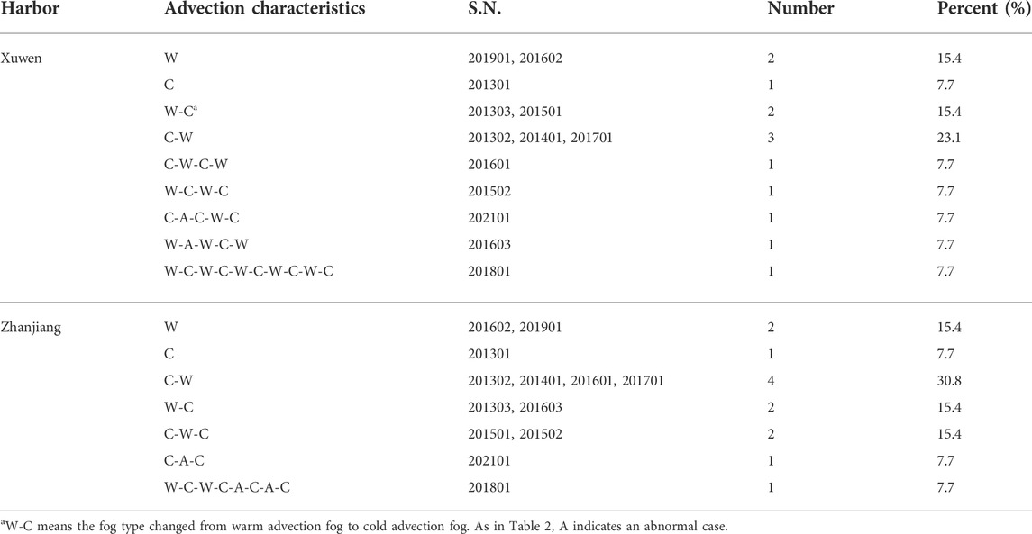
TABLE 3. Characteristics of advection fog process at both harbors for 2013–2021.

4 Feasibility of sea fog monitoring and early warning

4.1 Hourly backward trajectory distribution

Here, we use the incoming flow near the surface (10 m level) to calculate the hourly backward-trajectory frequency distribution. For both harbors, as time goes back, the high-frequency region moves from the port to the east (Figures 6–8). However, 3 h before the sea fog formed (t = −3), a clear and complete high-frequency center affects Xuwen port, but the high-frequency centers affecting Zhanjiang port are dispersed (Figure 6).

FIGURE 6

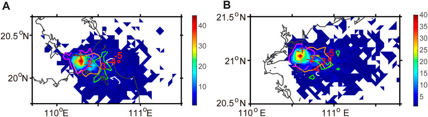
FIGURE 6. Superimposed hourly backward trajectory frequency distribution from 1 h before the onset of sea fog (t = −1) to 6 h before (t = −6). (A) Xuwen harbor. (B) Zhanjiang harbor. Shaded parts show the hourly frequency overlaid (but not accumulated) of each grid from t = −1 to t = −6. Contours are the isoline for frequency of at least five per hour at times t = −1 (pink), t = −2 (yellow), t = −3 (green), t = −4 (white), and t = −5 (red). For t = −6 the max frequency is less than 5. Numbers −1 to −5 are put at the geometric center of each isoline.

In general, as time goes back, the high-frequency region of the backward trajectory becomes more and more scattered. Graphically, within 4 h of the fog event, the high-frequency regional center of the two ports is still relatively obvious, and thus the single point monitoring method may be used for effective early warning of sea fog (Figures 7, 8). However, the results indicate more difficulty in reaching an advance of 5–6 h. In particular, for 6 h prior to the fog (t = −6), the central area of the high-frequency area is less than 5. Such a low value reflects a largely decentralized state, indicating that at this time, the backward trajectory incoming flow is very dispersed, making it difficult to use the single point monitoring method to for sea fog early warning (Figures 7, 8).

FIGURE 7

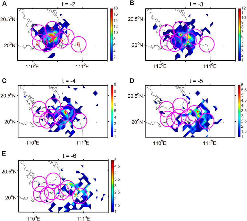
FIGURE 7. Proposed monitoring and early warning setup for Xuwen harbor. All eight visibility lidars, labeled and circled, are on the coast. Shading is the hourly backward-trajectory frequency distribution from (A) t = −2 h to (E) t = −6 h (indicate the advance time in hours) for Xuwen harbor. Pink circles are the effective radius of lidar (15 km). Positions 1–3 are built, positions 4-8 are proposed visibility lidars.

FIGURE 8

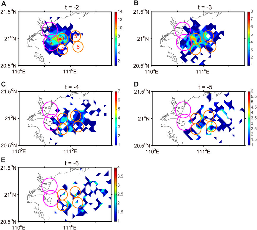
FIGURE 8. Same as Figure 7, but for Zhanjiang harbor. Numbers 1–6 are station locations: 1) and 2) are visibility lidars, 3) to 6) are buoys. Pink circles are the effective radius of the lidar (15 km), smaller brown circles are those for the buoys (10 km).

4.2 Early warning and monitoring scheme

Before the harbor authorities install a monitoring operation for early warning of impending sea fog, they should know which arrangement of instruments has the more likely chance of success. Here we use the calculated backward trajectory frequency, combined with knowledge of the local geography and monitoring range of the instruments, to propose monitoring and early warning schemes for the two harbors.

For Xuwen harbor, since the high-frequency area of sea fog is mainly in the south and the east side of Qiongzhou Strait, we suggest deploying more lidar along the south and east side of the strait. Here we assume that the effective range of the radar is 15 km. As there are presently three lidars (number 1–3) in this region, we propose adding five more (number 4–8) at the locations shown in Figure 7. Location selection is mainly based on backward trajectory, distance between locations and lidar coverage.

Because a 1 h warning may be too short, we mainly analyze the early warning ability of 2–6 h. According to this scheme, the early warning probabilities of sea fog in Xuwen harbor for 2, 3, and 4 h in advance are 87.50, 66.23, and 49.78% respectively. The probability then quickly drops to 36.40 and 25.22% for 5 and 6 h, respectively (Table 4). However, different locations have different sea fog warning probabilities. For example, for 2–3 h in advance, the probability at positions 4–6 (Figure 7) are the highest, whereas for 4 h in advance, the probability of positions 4, 6, and seven are the highest. As positions 1–3 are visibility lidars already built, it is necessary to build the position 4–8 visibility lidars for more effective early warning (Table 5).

TABLE 4

TABLE 4. Sea-fog detection percentage.

TABLE 5

TABLE 5. Sea fog detection percentage for Xuwen harbor.

For Zhanjiang harbor, because the main incoming flow comes from the sea on the east side, we suggest a monitoring and early warning scheme with visibility lidars in positions 1-2 and four buoys in positions 3–6 (Figure 8). We assume that the radius represented by each buoy’s observation is 10 km. To determine the lidar locations, we seek to have them spaced as far apart as possible, yet have each one in a region where the fog-producing trajectories pass. The selection of four buoy locations are a little more complicated. First, we select the initial locations by the same criteria as that for the lidar positions. This gives four initial locations. Second, a grid within a 20 km radius of each initial location is used for further statistical discrimination. Third, when several points have the same number of back trajectories, we choose the location with the highest probability at the first 4 hours.

With such an instrument setup, the early warning probabilities of sea fog in Zhanjiang harbor for 2, 3, and 4 h in advance are 83.77, 64.47, and 47.15% respectively. Similar to the Xuwen case, the probability quickly drops to 30.70 and 20.61% for 5 and 6 h, respectively (Table 4). As for the exact probability, for 2 h in advance, the probability of positions 1–3 are highest, whereas for 3–4 h in advance, positions 3–5 have the highest probability (Table 6).

TABLE 6

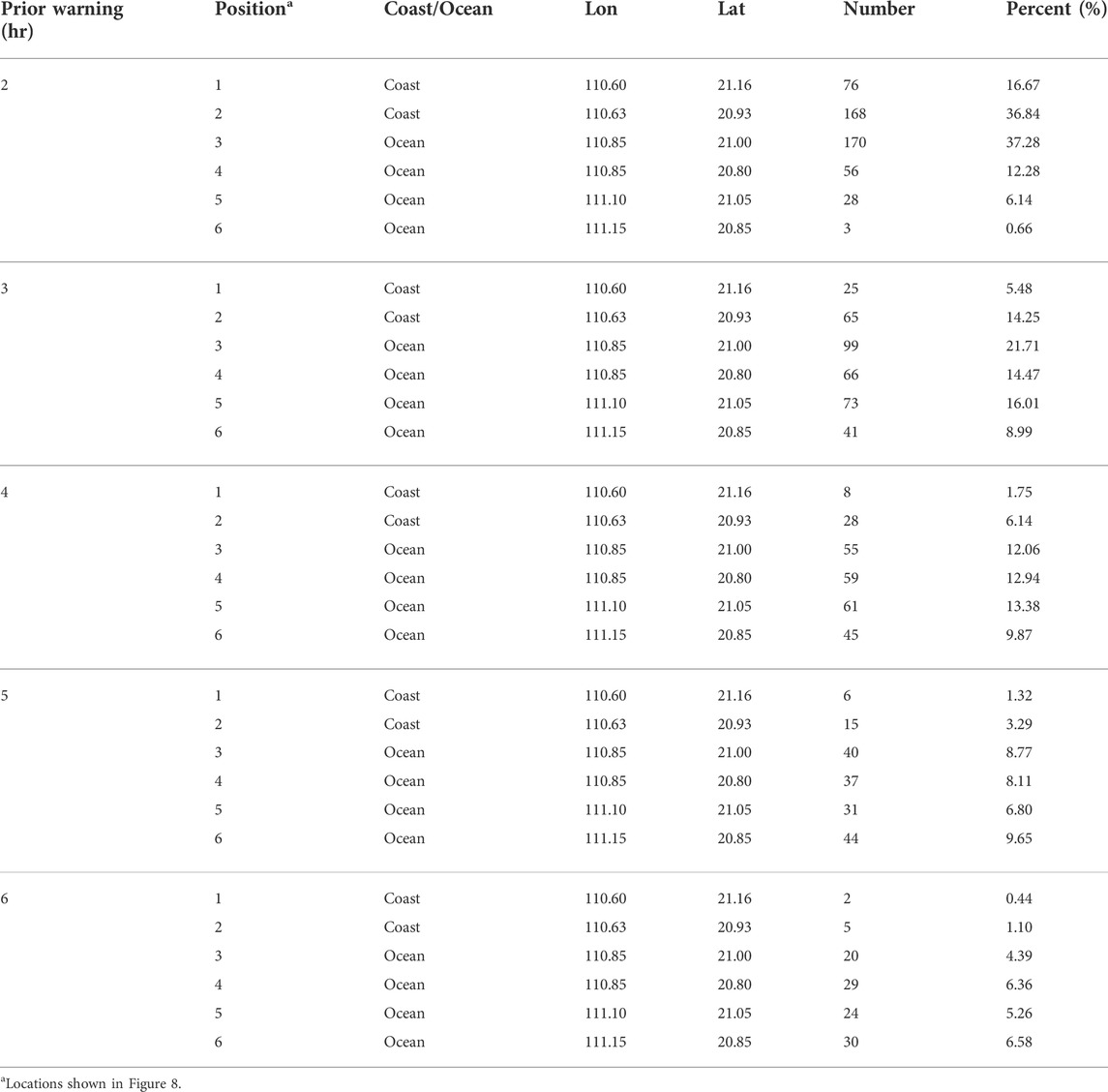
TABLE 6. Same as Table 5, but for Zhanjiang harbor.

Based on the above analysis and our review of previous daily sea fog early warning and prediction methods, we propose an operational sea fog early warning and monitoring scheme for the two harbors. We also argue that effective sea fog early warning and monitoring requires good cooperation between the Meteorological Bureau and the maritime safety administration (Figure 9).

FIGURE 9

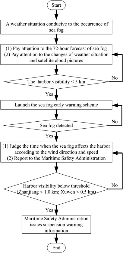
FIGURE 9. Flow chart of the early warning and monitoring scheme.

5 Conclusion and discussion

In this study, we focused on the feasibility of a system for sea fog monitoring and early warning at Xuwen and Zhanjiang harbors on the South China Sea. We selected 13 sea fog events that occurred at both harbors that lasted for at least 3 days in the period 2013–2021. First, we ran a multi-layer 72 h backward trajectory analysis. Second, we analyzed the proportion of events that were either cold or warm advection fog cases. Finally, based on our analysis of the 10 m incoming flow, we proposed a measurement system for each harbor that would provide a sea fog early warning as well as a monitor for the sea fog. The main conclusions are as follows:

(1) For both harbors, the direction of incoming flow changed clockwise from northeast to west as the height increased from low to high. The main difference in incoming flow between the harbors was in the lower layer. In this layer, the primary directions to Zhanjiang harbor were from north, northeast and east-northeast, whereas for Xuwen, the directions were from east, southeast, and south.

(2) Based on low-level incoming flow and the heat flux analysis, the fog at Xuwen harbor was 49.56% warm advection fog and 48.03% cold advection fog cases. For Zhanjiang harbor, the cases were 37.06% warm advection fog and 58.33% cold advection fog. Xuwen harbor has 12.5% more warm advection fog cases and 10.3% fewer cold advection fog cases than that in Zhanjiang harbor.

(3) We proposed monitoring and early warning setups for each harbor. For Xuwen, we suggested eight visibility lidars located on the north and south sides of Qiongzhou Strait. This setup gave early warning probabilities of sea fog for 2, 3, and 4 h in advance of 87.50, 66.23, and 49.78% respectively. For Zhanjiang harbor, we suggested two visibility lidars and four buoys at the east side of the harbor. This setup gave early warning probabilities of sea fog for 2, 3, and 4 h in advance of 83.77, 64.47, and 47.15%. For 5–6 h in advance, the early warning probabilities of both harbors drop quickly.

Although the distance between the two harbors is only about 100 km, each has different near surface flow that results in different types of advection fog. We believe that these differences may come from local geographical and climatic characteristics, submarine topography, SST distribution characteristics, and local air–sea and land–air interactions (Koračin et al., 2014; Koračin and Dorman, 2017).

Methods of monitoring and early warning of sea fog need further improvement. First, we should use the direct, observed SAT and SST data (not the present indirect methods via low-level incoming flow and heat flux analysis) to reduce uncertainty in the classification of the two types of advection fog. Second, the selection of monitoring points may be improved, especially the locations at sea. Third, the flow chart of sea fog early warning and monitoring still needs to be improved in practice.

How to further strengthen the monitoring and early warning of sea fog in the future? We believe that the first is to build a unified sea fog monitoring and early warning center in each harbor. The second is to strengthen the complementarity of coastal monitoring, marine monitoring, and satellite monitoring, which will help to improve the accuracy and timeliness of sea fog early warning. In the future, we will strengthen our work in this area.

Data availability statement

The original contributions presented in the study are included in the article/supplementary material, further inquiries can be directed to the corresponding author.

Author contributions

MZ: Formal analysis; Methodology and software; Writing–original draft. HH: Conceptualization; Supervision; Writing–review and editing. HL: Data Curation; Resources. JC: Data Curation; Resources. DW: Data Curation; Resources. XZ: Data Curation; Resources.

Funding

This study was supported jointly by the National Natural Science Foundation of China (Grant Nos. 42275083 and 41675021), the Key Meteorological Sciences Research Project (Grant No. GRMC 2020Z01), and the Innovation team of severe weather mechanism and forecasting technology in the South China Sea of the Guangdong Provincial Meteorological Bureau.

Acknowledgments

Special thanks to the crew of the Xuwen County Meteorological Bureau, for their help in collecting the data.

Conflict of interest

The authors declare that the research was conducted in the absence of any commercial or financial relationships that could be construed as a potential conflict of interest.

Publisher’s note

All claims expressed in this article are solely those of the authors and do not necessarily represent those of their affiliated organizations, or those of the publisher, the editors and the reviewers. Any product that may be evaluated in this article, or claim that may be made by its manufacturer, is not guaranteed or endorsed by the publisher.

References

Ballard, S. P., Golding, B. W., and Smith, R. N. B. (1991). Mesoscale model experimental forecasts of the haar of northeast Scotland. Mon. Wea. Rev. 119, 2107–2123. doi:10.1175/1520-0493(1991)119<2107:MMEFOT>2.0.CO;2

CrossRef Full Text | Google Scholar

Bendix, J. (1995). A case study on the determination of fog optical depth and liquid water path using AVHRR data and relations to fog liquid water content and horizontal visibility. Int. J. Remote Sens. 16, 515–530. doi:10.1080/01431169508954416

CrossRef Full Text | Google Scholar

Bendix, J., Thies, B., Nauss, T., and Cermak, J. (2006). A feasibility study of daytime fog and low stratus detection with TERRA/AQUA-MODIS over land. Meteorol. App. 13, 111–125. doi:10.1017/s1350482706002180

CrossRef Full Text | Google Scholar

Chen, C., Zhang, M., Perrie, W., Chang, R., Chen, X., Duplessis, P., et al. (2020a). Boundary layer parameterizations to simulate fog over Atlantic Canada waters. Earth Space Sci. 7, e2019EA000703. doi:10.1029/2019EA000703

CrossRef Full Text | Google Scholar

Chen, Y., Cai, Q. B., Xu, W. J., Xian, J. H., Li, X., Zhang, C. H., et al. (2020b). Application of visibility lidar in a heavy fog in Qiongzhou Strait. Adv. Meteorological Sci. Technol. 10 (4), 128–132. doi:10.3969/j.issn.2095-1973.2020.04.023

CrossRef Full Text | Google Scholar

Compilation group of Guangdong Meteorological Bureau (2006). Technical guidance on weather forecasting in Guangdong. Province, Beijing: China Meteorological Press, 526pp.

Google Scholar

Dorman, C. E., Mejia, J., Koračin, D., and McEvoy, D. (2019). World marine fog analysis based on 58-years of ship observations. Int. J. Climatol. 40, 145–168. doi:10.1002/joc.6200

CrossRef Full Text | Google Scholar

Draxler, R. R., and Hess, G. D. (1998). An overview of the HYSPLIT_4 modeling system for trajectories, dispersion, and deposition. Aust. Meteor. Mag. 47, 295–308.

Google Scholar

Findlater, J., Roach, W. T., and Mchugh, B. C. (1989). The haar of north-east Scotland. Q. J. R. Meteorol. Soc. 115, 581–608. doi:10.1002/qj.49711548709

CrossRef Full Text | Google Scholar

Fleming, Z. L., Monks, P. S., and Manning, A. J. (2012). Review: Untangling the influence of air-mass history in interpreting observed atmospheric composition. Atmos. Res. 104–105, 1–39. doi:10.1016/j.atmosres.2011.09.009

PubMed Abstract | CrossRef Full Text | Google Scholar

Fu, G., Guo, J., Xie, S., Duan, Y., Zhang, T., and Wang, J. (2006). Analysis and high-resolution modeling of a dense sea fog event over the Yellow Sea. Atmos. Res. 81, 293–303. doi:10.1016/j.atmosres.2006.01.005

CrossRef Full Text | Google Scholar

Gao, S. H., Lin, H., Shen, B., and Fu, G. (2007). A heavy sea fog event over the Yellow Sea in March 2005: Analysis and numerical modeling. Adv. Atmos. Sci. 24 (1), 65–81. doi:10.1007/s00376-007-0065-2

CrossRef Full Text | Google Scholar

Gultepe, I., Tardif, R., Michaelides, S. C., Cermak, J., Bott, A., Bendix, J., et al. (2007). Fog research: A review of past achievements and future perspectives. Pure Appl. Geophys. 164, 1121–1159. doi:10.1007/s00024-007-0211-x

CrossRef Full Text | Google Scholar

Han, L. G., Long, J. C., Xu, F., and Xu, J. J. (2022). Decadal shift in sea fog frequency over the northern South China Sea in spring: Interdecadal variation and impact of the Pacific Decadal Oscillation. Atmos. Res. 265, 105905. doi:10.1016/j.atmosres.2021.105905

CrossRef Full Text | Google Scholar

Heo, K. Y., and Ha, K. J. (2010). A coupled model study on the formation and dissipation of sea fogs. Mon. Weather Rev. 138 (4), 1186–1205. doi:10.1175/2009mwr3100.1

CrossRef Full Text | Google Scholar

Hersbach, H., Bell, B., Berrisford, P., Hirahara, S., Horanyi, A., Munoz‐Sabater, J., et al. (2020). The ERA5 global reanalysis. Q. J. R. Meteorol. Soc. 146, 1999–2049. doi:10.1002/qj.3803

CrossRef Full Text | Google Scholar

Huang, B., Liu, C., Banzon, V., Freeman, E., Graham, G., Hankins, B., et al. (2021). Improvements of the daily optimum interpolation sea surface temperature (DOISST) version 2.1. J. Clim. 34, 2923–2939. doi:10.1175/jcli-d-20-0166.1

CrossRef Full Text | Google Scholar

Huang, H. J., Huang, B., Yi, L., Liu, C. X., Tu, J., Wen, G. H., et al. (2019). Evaluation of the global and regional assimilation and prediction system for predicting sea fog over the South China Sea. Adv. Atmos. Sci. 36 (6), 623–642. doi:10.1007/s00376-019-8184-0

CrossRef Full Text | Google Scholar

Huang, H. J., Liu, H. N., Huang, J., Mao, W. K., and Bi, X. Y. (2015). Atmospheric boundary layer structure and turbulence during sea fog on the southern China coast. Mon. Weather Rev. 143 (5), 1907–1923. doi:10.1175/mwr-d-14-00207.1

CrossRef Full Text | Google Scholar

Huang, H. J., Liu, H. N., Jiang, W. M., Huang, J., and Mao, W. K. (2011). Characteristics of the boundary layer structure of sea fog on the coast of southern China. Adv. Atmos. Sci. 28 (6), 1377–1389. doi:10.1007/s00376-011-0191-8

CrossRef Full Text | Google Scholar

Huang, H. J., Zhan, G. W., Liu, C. X., Tu, J., and Mao, W. K. (2016). A case study of numerical simulation of sea fog on the southern China coast. J. Trop. Meteorology 22 (4), 497–507. doi:10.16555/j.1006-8775.2016.04.005

CrossRef Full Text | Google Scholar

Kamangir, H., Collins, W., Tissot, P., King, S. A., Dinh, H. T. H., Durham, N., et al. (2021). FogNet: A multiscale 3D CNN with double-branch dense block and attention mechanism for fog prediction. Mach. Learn. Appl. 5, 100038. doi:10.1016/j.mlwa.2021.100038

CrossRef Full Text | Google Scholar

Kim, C. K., and Yum, S. S. (2012). A numerical study of sea fog formation over cold sea surface using a one-dimensional turbulence model coupled with the weather research and forecasting model. Bound. Layer. Meteorol. 143 (3), 481–505. doi:10.1007/s10546-012-9706-9

CrossRef Full Text | Google Scholar

Koračin, D., Businger, J. A., Dorman, C. E., and Lewis, J. M. (2005). Formation, evolution, and dissipation of coastal sea fog. Bound. Layer. Meteorol. 117, 447–478. doi:10.1007/s10546-005-2772-5

CrossRef Full Text | Google Scholar

Koračin, D., Dorman, C. E., Lewis, J. M., Hudson, J. G., Wilcox, E. M., and Torregrosa, A. (2014). Marine fog: A review. Atmos. Res. 143, 142–175. doi:10.1016/j.atmosres.2013.12.012

CrossRef Full Text | Google Scholar

Koračin, D., and Dorman, C. (2017). “Marine fog: Challenges and advancements in observations, modeling, and forecasting,” in Springer atmospheric sciences (Switzerland: Springer International Publishing), 537.

Google Scholar

Koračin, D., Lewis, J., Thompson, W. T., Dorman, C. E., and Businger, J. A. (2001). Transition of stratus into fog along the California coast: Observations and modeling. J. Atmos. Sci. 58 (13), 1714–1731. doi:10.1175/1520-0469(2001)058<1714:tosifa>2.0.co;2

CrossRef Full Text | Google Scholar

Lee, T. F., Turk, F. J., and Richardson, K. (1997). Stratus and fog products UsingGOES-8–93.9-μm data. Wea. Forecast. 12, 664–677. doi:10.1175/1520-0434(1997)012<0664:safpug>2.0.co;2

CrossRef Full Text | Google Scholar

Leipper, D. F. (1994). Fog on the U. S. West coast: A review. Bull. Amer. Meteor. Soc. 75 (2), 229–240. doi:10.1175/1520-0477(1994)075<0229:fotuwc>2.0.co;2

CrossRef Full Text | Google Scholar

Lewis, J. M., Koračin, D., and Redmond, K. T. (2004). sea fog research in the United Kingdom and United States: A historical essay including outlook. Bull. Amer. Meteor. Soc. 85, 395–408. doi:10.1175/bams-85-3-395

CrossRef Full Text | Google Scholar

Maritime Safety Administration of the Ministry of transport of China (2019). Analysis of water traffic safety situation in 2018. China Marit. Saf. 5, 32–33. doi:10.16831/j.cnki.issn1673-2278.2019.05.015

CrossRef Full Text | Google Scholar

Petterssen, S. (1938). On the causes and the forecasting of the California fog. Bull. Am. Meteorol. Soc. 19, 49–55. doi:10.1175/1520-0477-19.2.49

CrossRef Full Text | Google Scholar

Pilié, R. J., Mack, E. J., Rogers, C. W., Katz, U., and Kocmond, W. C. (1979). The formation of marine fog and the development of fog-stratus systems along the California coast. J. Appl. Meteor. 18, 1275–1286. doi:10.1175/1520-0450(1979)018<1275:tfomfa>2.0.co;2

CrossRef Full Text | Google Scholar

Stein, A. F., Draxler, R. R., Rolph, G. D., Stunder, B. J. B., Cohen, M. D., and Ngan, F. (2015). NOAA’s HYSPLIT atmospheric transport and dispersion modeling system. Bull. Am. Meteorol. Soc. 96, 2059–2077. doi:10.1175/bams-d-14-00110.1

CrossRef Full Text | Google Scholar

Tachibana, Y., Iwamoto, K., Ogawa, H., Shiohara, M., Takeuchi, K., and Wakatsuchi, M. (2008). Observational study on atmospheric and oceanic boundary-layer structures accompanying the Okhotsk anticyclone under fog and non-fog conditions. J. Meteorological Soc. Jpn. 86, 753–771. doi:10.2151/jmsj.86.753

CrossRef Full Text | Google Scholar

Tanimoto, Y., Xie, S.-P., Kai, K., Okajima, H., Tokinaga, H., Murayama, T., et al. (2009). Observations of marine atmospheric boundary layer transitions across the summer Kuroshio Extension. J. Clim. 22, 1360–1374. doi:10.1175/2008jcli2420.1

CrossRef Full Text | Google Scholar

Tao, S. Y., and Chen, L. X. (1987). “A review of recent research on the east asian summer monsoon in China,” in Monsoon meteorology. Editors C. P. Chang, and T. N. Krishnamurti (Oxford: Oxford University Press), 60–92.

Google Scholar

Taylor, G. I. (1917). The formation of fog and mist. Q. J. R. Meteorol. Soc. 43, 241–268. doi:10.1002/qj.49704318302

CrossRef Full Text | Google Scholar

Tremant, M. (1987). “La prévision du brouillard en mer,” in Météorologie Maritime et Activities Océanographique Connexes (Geneva, Switzerland: World Meteorological Organization).

Google Scholar

Wang, B. H. (1985). sea fog. Beijing: China Ocean Press, 358pp.

Google Scholar

Wang, Y., Gao, S., Fu, G., Sun, J., and Zhang, S. (2014). Assimilating MTSAT‐derived humidity in nowcasting sea fog over the Yellow Sea. Weather Forecast. 29, 205–225. doi:10.1175/WAF‐D‐12‐00123.1

CrossRef Full Text | Google Scholar

Wilcox, E. M. (2017). “Multi-spectral remote sensing of sea fog with simultaneous passive infrared and microwave sensors,” in Marine fog: Challenges and advancements in observations, modeling, and forecasting. Editors D. Koračin, and C. Dorman (Switzerland: Springer International Publishing), 511–526.

CrossRef Full Text | Google Scholar

Xian, J. H., Sun, D. S., Amoruso, S., Xu, W. J., and Wang, X. (2020). Parameter optimization of a visibility LiDAR for sea-fog early warnings. Opt. Express 28, 23829–23845. doi:10.1364/oe.395179

PubMed Abstract | CrossRef Full Text | Google Scholar

Yang, D., Ritchie, H., Desjardins, S., Pearson, G., MacAfee, A., and Gultepe, I. (2010). High-resolution GEM-LAM application in marine fog prediction: Evaluation and diagnosis. Weather Forecast. 25, 727–748. doi:10.1175/2009waf2222337.1

CrossRef Full Text | Google Scholar

Yang, L., Liu, J. W., Ren, Z. P., Xie, S. P., Zhang, S. P., and Gao, S. H. (2018). Atmospheric conditions for advection-radiation fog over the Western Yellow Sea. J. Geophys. Res. Atmos. 123, 5455–5468. doi:10.1029/2017JD028088

CrossRef Full Text | Google Scholar

Yang, Y., Hu, X. M., Gao, S. H., and Wang, Y. M. (2019). Sensitivity of WRF simulations with the YSU PBL scheme to the lowest model level height for a sea fog event over the Yellow Sea. Atmos. Res. 215, 253–267. doi:10.1016/j.atmosres.2018.09.004

CrossRef Full Text | Google Scholar

Yuan, J. N., and Huang, J. (2011). An observational analysis and 3-dimensional numerical simulation of a sea fog event near the Pearl River Mouth in boreal spring. Acta Meteorol. Sin. 69 (5), 847–859. doi:10.11676/qxxb2011.074

CrossRef Full Text | Google Scholar

Zhang, S. P., and Lewis, J. M. (2017). in Chapter 6, synoptic processes, marine fog: Challenges and Advancements in observations, modeling, and forecasting. Editors D. Koračin, and C. E. Dorman (Cham: Springer International Publishing AG), 537pp. doi:10.1007/978-3-319-45229-6_6

CrossRef Full Text | Google Scholar

Zhang, S. P., Xie, S. P., Liu, Q. L., Yang, Y. Q., Wang, X. G., and Ren, Z. P. (2009). Seasonal variations of Yellow Sea fog: Observations and mechanisms. J. Clim. 22, 6758–6772. doi:10.1175/2009jcli2806.1

CrossRef Full Text | Google Scholar

Zhang, S. P., and Yi, L. (2013). A comprehensive dynamic threshold algorithm for daytime sea fog retrieval over the Chinese adjacent seas. Pure Appl. Geophys. 170, 1931–1944. doi:10.1007/s00024-013-0641-6

CrossRef Full Text | Google Scholar

Zhou, B. B., and Du, J. (2010). Fog prediction from a multimodel mesoscale ensemble prediction system. Weather Forecast. 25, 303–322. doi:10.1175/2009waf2222289.1

CrossRef Full Text | Google Scholar