A fast least-squares reverse time migration method using cycle-consistent generative adversarial network

With high imaging accuracy, high signal-to-noise ratio, and good amplitude balance, least-squares reverse time migration (LSRTM) is an imaging algorithm suitable for deep high-precision oil and gas exploration. However, the computational costs limit its large-scale industrial application. The difference between traditional reverse time migration (RTM) and LSRTM is whether to eliminate the effect of the Hessian operator or not while solving Hessian matrix explicitly or eliminating the effect of the Hessian matrix implicitly has a very high requirement on computation or storage capacity. We simulate the inverse Hessian by training a cycle-consistent generative adversarial network (cycleGAN) to construct a mapping relationship between the RTM results and the true reflectivity models. The trained network is directly applied to the RTM imaging results, which improves the imaging quality while significantly reducing the calculation time. We select three velocity models and two velocity models respectively to generate the training and validation data sets, where the validation data is not involved in the training process. The prediction results on the validation data sets show that the trained network significantly improves the imaging quality with almost no additional in computational effort. Finally, we apply the network trained with only synthetics to the field data. The predicted results confirm the effectiveness and good generalization of the proposed method.

Introduction

For the high-precision imaging problem of complex geological formations and deep reservoirs, the reverse time migration (RTM) based on the two-way wave-equation is considered to be a better imaging method (Baysal et al., 1983; Chang, 1987). Essentially, RTM is only the conjugate transpose of the forward operator, not its inverse (Lailly, 1983). Therefore, influenced by the limited acquisition aperture, complex subsurface structure, and limited seismic wave bandwidth, the RTM results suffer from migration noise, non-uniform illumination, and insufficient resolution (Cheng et al., 2021), which prevents it from imaging deep and unconventional oil and gas reservoirs finely. In addition, conventional RTM can only image the subsurface discontinuities while the accurate amplitude information of the real formation lithology changes can not be guaranteed (Chen and Zhang, 2012).

To eliminate the effect of the Hessian matrix, the imaging problem of RTM can be solved as a least-squares inverse problem to suppress the migration noise, increase the resolution, and improve the amplitude fidelity, which is the least-squares reverse time migration (Tarantola, 1987; Chavent and Plessix, 1999; Nemeth et al., 1999; Valenciano et al., 2006). The least-squares reverse time migration (LSRTM) can be solved in model space (Hu et al., 2001; Rickett, 2003; Guitton, 2004) or in data space (Tarantola, 1987; Schuster, 1993; Chavent and Plessix, 1999; Nemeth et al., 1999). The LSRTM in model space requires solving the Hessian matrix explicitly and using its inverse to deblurring the RTM imaging results. Directly solving the full Hessian matrix in practical applications is extremely demanding in terms of computation and storage (Tang, 2009). Therefore, some researchers have proposed that the Hessian matrix can be approximated as a diagonal matrix under the assumption of high-frequency asymptotics and infinite aperture (Beylkin, 1985; Chavent and Plessix, 1999; Plessix and Mulder, 2004; Symes, 2008). However, this approximation is not suitable for the limited frequency range and acquisition geometry, and the Hessian matrix in this case is no longer diagonally dominant (Pratt et al., 1998; Chavent and Plessix, 1999; Plessix and Mulder, 2004; Valenciano et al., 2006). In regions below the high-velocity body or salt dome where illumination is lacking, the energy on the diagonal of the Hessian matrix is scattered along the non-diagonal direction (Albertin et al., 2004; Valenciano, 2008). Therefore, the diagonal Hessian matrix is of limited use for deblurring the migration imaging results, especially in regions with severe energy attenuation of seismic waves. Some non-diagonal elements of the Hessian matrix can be properly computed to compensate for the illumination unevenness in regions with severe absorption attenuation and enhance the deblurring effect (Albertin et al., 2004; Valenciano, 2008). However, solving the non-diagonal elements of the matrix will significantly increase the computational effort.

The LSRTM in data space is used to find the reflectivity model that best matches the observed seismic data by iterative algorithms such as the steepest descent method and the conjugate gradient method (Nemeth et al., 1999). Instead of solving the huge Hessian matrix directly, this approach implicitly removes the effect of the Hessian matrix by iteratively updating the reflectivity model. However, iterative solving causes a large amount of computation, and the convergence rate depends on suitable preconditioning constraints (Tang, 2009; Wu et al., 2021; Wu et al., 2022; Yao et al., 2022). To improve the computational efficiency of LSRTM, one approach is to compress the massive shot data into several super gathers to reduce the computational effort, which is the multisource migration method (Romero et al., 2000). To suppress the multi-source crosstalks, some researchers proposed the shot encoding techniques, such as amplitude encoding (Hu et al., 2016), phase encoding (Schuster et al., 2011; Li et al., 2014; Li et al., 2017) and plane wave encoding (Zhang et al., 2005; Dai and Schuster, 2013; Li et al., 2018). These schemes reduce the correlation of crosstalk noise in the imaging results of different super gathers by constructing suitable encoding functions and finally stack the imaging results to suppress the noise (Etgen, 2005; Zhang et al., 2005). However, when the observation system is not fixed, the source wavefield of the multisource forward simulation and the super gather synthesized from the observation data cannot be matched, resulting in slow convergence (Li et al., 2018). Liu and Peter (2018) propose a one-step LSRTM method to design a deblurring preconditioner using the Wiener filter, reducing the computational effort to twice the RTM. In summary, LSRTM in model space requires certain calculations and significant storage costs to solve the Hessian matrix explicitly, while LSRTM in data space requires a large amount of computation to solve the reflectivity iteratively and does not require much storage.

In recent years, with the popularity of artificial intelligence, many researchers introduced deep learning techniques to solve geophysical problems such as fault segmentation (Wu et al., 2019), seismic data denoising (Yu et al., 2019; Saad and Chen, 2020), and first-arrival picking (Hu et al., 2019; Duan and Zhang, 2020). These solutions use techniques such as DNN, CNN, RNN, etc. These networks can be broadly classified into two categories based on the application scenarios: discriminative models that solve classification, identification, or localization problems, and generative models that solve the mapping relationship between data from two different domains. The generative adversarial network (GAN) combines the advantages of both types of networks by using a generative model to produce data from another domain and then using a discriminative model to evaluate the generated data (Goodfellow et al., 2014). Through adversarial training, GAN achieves state-of-the-art in solving the problem of style transfer between data from different domains. The cycleGAN (Zhu et al., 2017) consists of two GANs that ensure the structural consistency of the input and output data through cyclic consistency, taking full advantage of the mapping relationship between the source and target domain data. This network structure is well suitable for transferring the RTM data into a true reflectivity model and eliminating the blurring effect of Hessian matrix.

In this study, we propose to approximate the inverse Hessian by using cycleGAN for the deblurring purpose. The cycleGAN is trained by generating data sets of RTM imaging results with reflectivity models. The trained network is directly applied to the migration images to output high-quality imaging profiles. The training stage of the network consumes a certain computational effort and has an almost negligible computational cost. The proposed method is validated on both synthetic data and field data.

Methodology

Migration theory

For a given reflectivity model $m$ and a forward modeling operator $L$ , the observed data $d$ can be expressed as:

$d=Lm.(1)$

The goal of seismic imaging is to find the exact $m$ to fit the observed data $d$. Conventional reverse time migration can be expressed as:

$m_{mig}=L^{T}d,(2)$

where $m_{mig}$ is the matrix representation of the reverse time migration imaging result and $L^T$ is the matrix representation of the RTM operator. The $L^T$ is only the transpose of the forward operator, not its inverse, and cannot completely reverse the seismic wave propagation, so the migrated images of reverse time migration do not accurately represent the true reflectivity model.

The solution of the true reflectivity model $m$ can be solved in a least-squares framework. We define the misfit function $f\left(m\right)$ as follows:

$f\left(m\right)=\frac{1}{2}{\Vert Lm-d\Vert }^2.(3)$

Applying the transpose forward operator $L^T$ to both sides of Eq. 1, Eq. 4 is derived as follows:

$L^{T}d=L^{T}Lm.(4)$

Therefore, the precise least-squares solution of the reflectivity model $m$ can be obtained by:

$m={\left(L^{T}L\right)}^{-1}{L}^{T}d,(5)$

where ${\left(L^{T}L\right)}^{-1}$ is the inverse of the Hessian matrix, and $L^{T}d$ is the images of the reverse time migration. The relationship between the RTM imaging result and the true reflectivity model can be expressed as:

$m=H^{-1}{m}_{mig}.(6)$

Analysis of Hessian matrix

The expression of the conventional two-dimensional acoustic wave equation is:

$({\nabla }^2+{\omega }^2{\sigma }^2)u(x_s,x,\sigma ,\omega )=-f(x_s,\omega ),(7)$

where $\sigma \left(x\right)=1/v\left(x\right)$ is the slowness field of the medium, $v\left(x\right)$ is the corresponding velocity field, and $f(x_s,\omega )$ is the representation of the source wavelet in the frequency domain, indicating that the source point is at $x_s$ and the angular frequency is $\omega$. Based on the assumption that the inverse problem is approximately linear, the expression of the Hessian matrix for this two-dimensional acoustic wave equation can be written in the following form:

$\begin{array}{l}H(x,y)={\displaystyle \sum _{x_s,x_r}{\displaystyle \int \mathrm{Re}\{{\omega }^4{\left|f_s\left(\omega \right)\right|}^{2}G(x_s,x,\omega )\times G^T(x_s,y,\omega )}}\\ \times G(x,x_r,\omega )G^T(y,x_r,\omega )\}d\omega ,\end{array}(8)$

where $G(x_s,x,\omega )$ is the Green’s function at the source side, $G(x,x_r,\omega )$ is the Green’s function at the receiver side, and $f_s\left(\omega \right)$ is the source signature. The Green’s function term reflects the illumination of the seismic wave during migration, while the source wavelet term has an impact on the imaging resolution.

According to Eq. 6, it can be seen that the RTM results are missing the deblurring filtering of the inverse Hessian matrix with respect to the real reflectivity models. And according to Eq. 8, it can be concluded that the wavelet term and the Green’s function term in the expression of the Hessian matrix affect the imaging resolution and wavefield propagation, respectively. Therefore, the migrated images of RTM exhibit low imaging resolution, uneven illumination, and migration noise due to the lack of the inverse Hessian filtering. By solving the inverse Hessian matrix and applying it to the imaging results of the RTM, the true reflectivity model can be obtained, which is the least-squares reverse time migration in the model space. Theoretically, the LSRTM in model space only requires a certain computational cost to compute the inverse of the Hessian matrix in advance, and then the true reflectivity model can be acquired quickly. However, it is shown that solving the Hessian matrix requires storing the Green’s function, which is very large in practical applications, especially for 3D seismic data. Another approach is the LSRTM in the data space, which is an iterative solution to continuously update the reflectivity model so that the error between the simulated and observed data reaches the desired value. The LSRTM in the data domain does not take into account the storage cost, but it is computationally intensive, about 2N times more than the conventional migration (N denotes the number of iterations). Moreover, the convergence of the LSRTM in data space is very slow without proper gradient preconditioning.

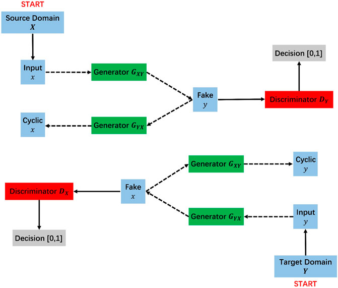
Our goal is to approximate the inverse of the Hessian matrix at a small cost. In the proposed method, we train cycleGAN to simulate the inverse Hessian and apply the trained network to process the RTM imaging data and play the role of the deblurring operator. First, we select some velocity models and generate the true reflectivity model $m$. Through finite-difference forward simulation, we can obtain the synthetic observation data $d=Lm$. Then, the RTM imaging of the observation data $d$ yields the migrated images $m_{mig}=L^{T}d$ after being filtered by the Hessian blurring operator. The source domain data $m_{mig}$ and the target domain data $m$ are fed into the network for training. According to Eq. 6, the trained network is the approximate inverse Hessian. After training, we apply the network to the new RTM imaging data to quickly obtain the least-squares solution in Eq. 5.

Network and loss function

The architecture of cycleGAN

GAN was proposed by Goodfellow et al. (2014), and it has good applicability to the problem of the source-to-target domain transformation. Conventional neural networks are used to find an optimal mapping relationship from input to output by backpropagation algorithms. The nature of the network can be viewed as a complex higher-order polynomial. GAN generally consists of two parts of the network, one as a generator and the other as a discriminator. During the training process of the network, the generator acts as a regular neural network, converting the input into data similar to the label, while the discriminator takes the output data of the generator as input and tries to distinguish the generated data from the real data in the training sets. Through this adversarial training, both the generator and the discriminator are continuously optimized, and eventually, we get the desired generator as a prediction network.

CycleGAN consists of 2 mirror-symmetric networks $GAN(G_{XY},G_{YX},D_Y)$ and $GAN(G_{YX},G_{XY},D_X)$, which together form a cycle network. As shown in Figure 1, cycleGAN has 2 discriminators $D_X$ and $D_Y$, and shares two generators $G_{XY}$ and $G_{YX}$. A sample $x$ from the data distribution $X$ in the source domain is input to the first network $GAN(G_{XY},G_{YX},D_Y)$, and fake $y$ and cyclic $x$ are produced by generators $G_{XY}$ and $G_{YX}$ in turn, then, fake $y$ enters the discriminator $D_Y$ to be identified as true or false. Similarly, for any sample $y$ in the data distribution $Y$ in the target domain, it can also be used as input to train the second network $GAN(G_{YX},G_{XY},D_X)$. The generator consists of an encoder, a converter, and a decoder. As shown in Figure 2, the encoder-decoder structure is similar to most convolutional neural networks, with convolutional and deconvolutional layers for feature extraction and reduction, and the converter structure is implemented by a multilayer Resnet. The discriminator is presented in Figure 3, which is implemented by a basic convolutional neural network, whose discriminating image requires extracting features from the input and finally adding a one-dimensional output convolutional layer to determine whether the extracted features belong to a specific class.

FIGURE 1

FIGURE 1. The architecture of cycleGAN.

FIGURE 2

FIGURE 2. The specific structure of the generator, consists of 2 convolutional layers forming the encoder, 7 Resnet blocks as the converter, and 2 deconvolutional layers as the decoder.

FIGURE 3

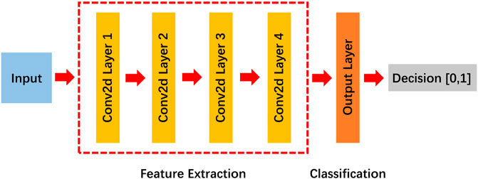
FIGURE 3. The detailed architecture of the discriminator, 4 convolutional layers are used to extract the features of the input data, and finally, a convolutional layer is added to output the discriminant score.

Loss function analysis

The loss function is a measure of how good the output of the network is, and it is also the basis for correcting the tensor gradient in the backpropagation process. For a given size training batch, assuming the data distribution of the source domain is $p_x$ and the data distribution of the target domain is $p_y$, the data distribution of each training data $x$ and $y$ can be denoted as $x\sim p_x$ and $y\sim p_y$. The mathematical expectation of the training data can be expressed as $E_{x\sim P_x}$ and $E_{y\sim P_y}$. Therefore, the objective function of a conventional GAN can be expressed as (Goodfellow et al., 2014; Benaim and Wolf, 2017; Zhu et al., 2017):

$\begin{array}{l}{L}_{GAN}(G_{XY},D_Y,X,Y)=E_{y\sim P_y}\left[\log D_Y\left(y\right)\right]\\ +E_{x\sim P_x}\left[\log (1-D_Y\left(G\left(x\right)\right))\right].\end{array}(9)$

During training, the generator $G_{XY}$ tries to generate $G_{XY}\left(x\right)$ that is more similar to the reflectivity model, while the discriminator $D_Y$ tries to distinguish the generated $G_{XY}\left(x\right)$ from the real reflectivity model $y$ in the target domain. Thus, the goal of the generator is to minimize the objective function, while the discriminator tries to maximize it. For the first GAN, the final goal is ${\min }_G{\max }_{D_Y}{L}_{GAN}(G_{XY},D_Y,X,Y)$, and similarly, for the other GAN, its target is ${\min }_G{\max }_{D_X}{L}_{GAN}(G_{YX},D_X,Y,X)$.

By the above constraint of the objective function, GAN can theoretically map any data from the source domain to the target domain. However, only this constraint may result in the generator just generating a result with reflectivity characteristics, while the structural content is not the same as the source domain data. That is, only style transfer is achieved by training, and there is no guarantee that the content does not change. For any source domain data $x$, we need to guarantee $x\to G_{XY}\left(x\right)\to G_{YX}\left(G_{XY}\left(x\right)\right)\approx x$, which is also called forward cycle consistency. Similarly, for any target domain data $y$, we need it to satisfy the backward cycle consistency: $y\to G_{YX}\left(y\right)\to G_{XY}\left(G_{YX}\left(y\right)\right)\approx y$. Therefore, cycleGAN introduces a cyclic consistency error function as follows (Zhu et al., 2017):

$\begin{array}{l}{L}_{cycle}(G_{XY},G_{YX})=E_{x\sim P_x}\left[{\Vert G_{YX}\left(G_{XY}\left(x\right)\right)-x\Vert }_1\right]\\ +E_{y\sim P_y}\left[{\Vert G_{XY}\left(G_{YX}\left(y\right)\right)-y\Vert }_1\right],\end{array}(10)$

With the above loss function constraint, any data in the source or target domain can be effectively restored to the original data features in the end after two generator cycles. However, when the network is trained for application, the situation that the style completes the migration but the content changes still occurs. The analysis shows that only one generator is used as the prediction network when applied, and the cyclic consistency error function does not impose constraints on the intermediate variables. Therefore, we introduce the identity loss function to constrain the intermediate variables, and its expression is (Taigman et al., 2016; Benaim and Wolf, 2017; Zhu et al., 2017):

$\begin{array}{l}{L}_{identity}(G_{XY},G_{YX})=E_{y\sim P_y}\left[{\Vert \left(G_{XY}\left(y\right)\right)-y\Vert }_1\right]\\ +E_{x\sim P_x}\left[{\Vert \left(G_{YX}\left(x\right)\right)-x\Vert }_1\right].\end{array}(11)$

Therefore, the full loss function when training the cycleGAN is shown as follows:

$\begin{array}{l}L(G_{XY},G_{XY},D_X,D_Y)=L_{GAN}(G_{XY},D_Y,X,Y)\\ +L_{GAN}(G_{YX},D_X,Y,X)\\ +L_{cycle}(G_{XY},G_{YX})\\ +L_{identity}(G_{XY},G_{YX}).\end{array}(12)$

Data sets preparation and training

Training data sets production

As shown in Figures 4A–C, the Sigsbee2A model, SEAM model, and Pluto model are selected as the base models to produce the training data sets. The migrated images corresponding to the three models are generated by 2-8 finite-difference forward simulation and reverse time migration as shown in Figures 4D–F. Meanwhile, we produce the reflectivity model based on the velocity model as shown in Figures 4H–J. Considering the large band range variability between the reflectivity model and the migration imaging results, we adopt the convolution approach and conduct it with the reflectivity and the Ricker wavelet as the target domain data. Finally, we apply data enhancement such as cropping and resampling to generate 300 pairs of training data. Some of the training data are shown in Figure 5. The first row shows the RTM imaging data in the source domain, and the second row shows the convolution results in the target domain.

FIGURE 4

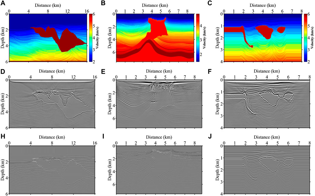
FIGURE 4. Three velocity models for producing training data sets in the source and target domains. (A) Sigsbee2A velocity model, (B) SEAM velocity model, and (C) Pluto velocity model. The corresponding RTM imaging results (D–F) and reflectivity models (H–J) for making the input and output samples respectively.

FIGURE 5

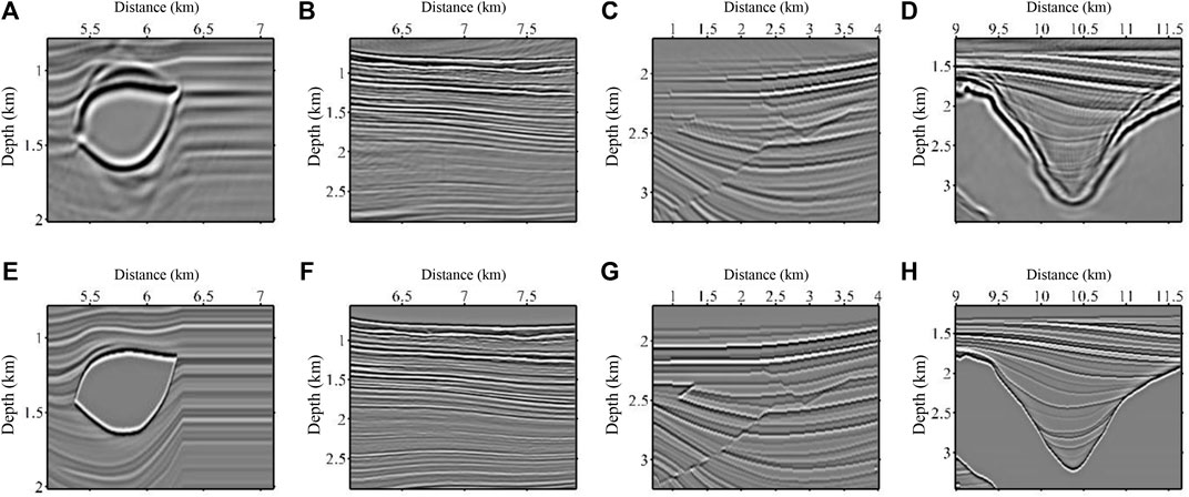
FIGURE 5. Four pairs of representative samples from the training data sets. The first row (A–D) are the migrated images in the source domain, and the second row (E–H) denotes the reflectivity in the target domain.

Training process

For $GAN(G_{XY},G_{YX},D_Y)$, the training first fixes the generator $G_{XY}$ and trains the discriminator $D_Y$ separately to improve the discriminator’s ability to identify the output results of the generator, and then fixes the discriminator $D_Y$ and trains the generator $G_{XY}$ individually to generate more realistic results and bypass the discriminator’s recognition. With this adversarial training approach, the ability of the generator $G_{XY}$ to map to the target domain can be greatly improved. Similarly, for the other $GAN(G_{YX},G_{XY},D_X)$, such adversarial training is also used. When the two GANs are trained for one epoch, the values of all loss functions are accumulated for backpropagation. Finally, the generator $G_{XY}$ is used as the expected prediction network for approximating the inverse Hessian matrix.

The number of epochs of the network training is set to 200 with a learning rate of 0.0002, which gradually decreased after the 100th epoch. The network is weighted with a cyclic consistency loss of 10 and the weight of the identity loss is set to 5. The training is based on the PyTorch platform, using a single NVIDIA RTX5000 GPU, and the total training time is 10 h.

Numerical tests on validation sets

BP 2.5D model

Figure 6A shows the BP2.5D velocity model with the reflectivity model shown in Figure 6B. We perform a finite-difference forward simulation of the velocity model in Figure 6A, then smooth the velocity model into migration velocity and perform reverse time migration to generate the imaging profile in Figure 6C. There are obvious low-frequency noise and acquisition footprints in the migrated image of the RTM, and the imaging energy is discontinuous in the region of violent tectonic undulations, meanwhile, the illumination is uneven on both sides of the model. We input the imaging result of Figure 6C into the trained network, and the obtained prediction result is shown in Figure 6D. The imaging quality in the predicted result is significantly improved, the surface acquisition footprints are eliminated very cleanly, and the low-frequency noise is well removed. The trained network compensates well for the uneven illumination in the migration result, and the overall imaging energy distribution is relatively uniform. It can be noted that the network is not completely accurate in predicting the result at the depth of 2 KM on the left side of the model since the imaging energy of the original RTM profile is very heterogeneous, resulting in the network not being able to predict it well. Figure 7 shows an enlarged view of the red dashed boxed area in Figure 6, with the first column showing the RTM imaging results, the second column denoting the network prediction results, and the third column representing the true reflectivity models. Comparing the first set of results (Figures 7A–C), it can be seen that the proposed method can better play the role of the deblurring operator and significantly improve the imaging quality. The second set of results (Figures 7D–F) shows that the trained network can not fully reduce the image of the RTM to the true reflectivity model, and it relies to some extent on the structure information of the original migration image, which differs from the real reflectivity model in some details, but generally maintains the consistency with the real reflectivity model.

FIGURE 6

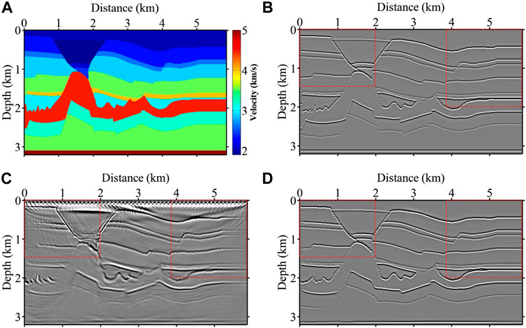
FIGURE 6. BP 2.5D velocity model (A) and the corresponding reflectivity model (B). Input the RTM imaging result (C) into the well-trained network, the prediction result is shown in (D).

FIGURE 7

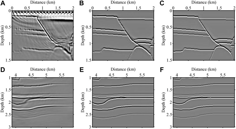
FIGURE 7. The zoom views of the red dashed boxed area in Figure 6. The first column represents the RTM results (A,D), the second column denotes the predictions (B,E) of the network and the third column is the true reflectivity model (C,F).

Marmousi model

Figure 8A shows the Marmousi velocity model, and Figure 8B shows its corresponding reflectivity model. The imaging result obtained after finite-difference simulation and reverse time migration of Figure 8A is shown in Figure 8C. The migrated image of RTM has more low-frequency noise in the shallow layer due to the blurring filtering of Hessian matrix. At the same time, the imaging resolution of the model bottom structure is low due to the influence of the deep high-speed layer shielding. Figure 8D shows the result of network prediction. Compared with Figure 8C, it can be concluded that the global resolution of the predicted imaging result is improved, and the reflection layer is finer. Most of the low-frequency noise in the shallow layer is removed, with a small amount of residual on both sides, and the trained network is also very clean for removing the acquisition footprints in the profile. The imaging quality of the deeper layers is also improved, however, some artifacts appear since some stray imaging energies in the result of the RTM are mistaken by the network as layers and recovered. Figure 9 shows an enlarged view of the red dashed boxed area in Figure 8. Figure 9A shows a shallow zoom of the RTM imaging result, where strong low-frequency noise and acquisition footprints exist within 0.5 KM of depth. These clutter energies are barely visible in the predicted result in Figure 9B, and the imaging energies at the interface are more converged. Comparing the second set of zooming results, it can be seen that the resolution of the result predicted by the network has improved significantly and the overall imaging energy is more balanced.

FIGURE 8

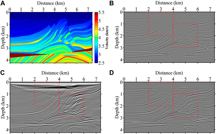
FIGURE 8. The Marmousi velocity model (A) and the corresponding reflectivity model (B). Input the RTM imaging result (C) into the well-trained network, the prediction result is shown in (D).

FIGURE 9

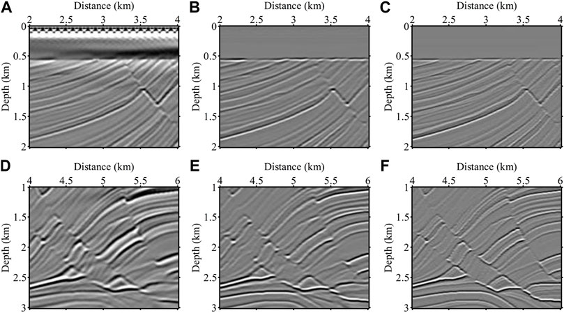
FIGURE 9. The zoom views of the red dashed boxed area in Figure 8. The first column represents the RTM results (A,D), the second column denotes the predictions (B,E) of the network and the third column is the true reflectivity model (C,F).

Field data test

We test the effectiveness of the proposed method with field data. We take the velocity model in Figure 10A as the migration velocity and perform the reverse time migration to obtain the imaging result shown in Figure 10B. We approximate the deblurring operator with the network previously trained on synthetic data, which acts directly on the migrated image of the field data. We input the migration result in Figure 10B into the network, and the prediction result output by the generator $G_{XY}$ is shown in Figure 10C. Compared with Figure 10B, there is a significant improvement in the resolution of the network prediction result, and a large amount of migration noise in the RTM image is well removed. Without damaging the effective signal, the surface acquisition footprints are eliminated very cleanly, and the shallow reflection layer is more obvious with more imaging details. However, the network does not handle the deep high steep structure very well. This is because the reflectivity model of our constructions is calculated along the depth direction. When the discretized model is small or not adequately sampled, its structure has poor continuity in the lateral direction. In contrast, the seismic wavefield propagates in all directions, and the imaging results have good continuity even on small models. Therefore, this results in an incompletely accurate mapping relationship between source-domain data and target-domain data, which affects the prediction results of the network.

FIGURE 10

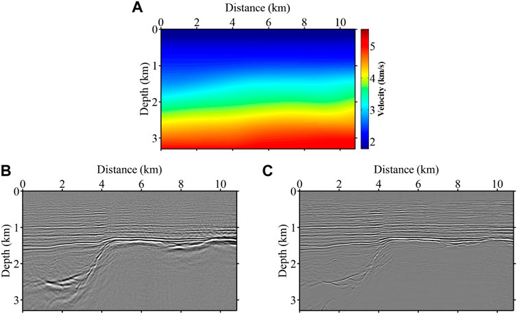
FIGURE 10. (A) migration velocity model, (B) RTM imaging result, and (C) the prediction result of the network trained only by synthetic data sets.

Conclusion

We propose a fast least-squares reverse time migration method based on cycleGAN. In the proposed method, cycleGAN is used to approximate the inverse Hessian matrix to play the role of a deblurring operator that acts directly on the RTM imaging results. By constructing a training data sets consisting of source domain data (migration imaging results) and target domain data (true reflectivity model), two GANs are trained separately from the two domains, and a generator mapping the source domain to the target domain is taken as the final prediction network after adversarial training. Synthetic data tests demonstrate the effectiveness of the proposed method in removing low-frequency noise, improving resolution, balancing illumination, and compensating for deep imaging energy. Applying the network trained only with synthetics directly to the field data, the prediction result shows that the proposed method has good generalization and good applicability to data sets with large variability. One point worth noting is that in the prediction result of the field data, the recovery of high steepness structures by the method is not very well. This problem can be solved by optimizing the label-making scheme and reducing the spatial sampling interval. Compared with the massive storage requirement of the Hessian matrix by the LSRTM in the model space, the storage demands of the proposed method are not high. Compared with the LSRTM in data space, the proposed method only consumes certain computational resources in the training stage and requires almost no computational costs in the prediction process.

Data availability statement

The raw data supporting the conclusions of this article will be made available by the authors, without undue reservation.

Author Contributions

YH and JH contributed to the idea and methodology, YH was responsible for the training data production, model and field data testing, and the writing of this manuscript, and YM checked and polished the manuscript. All authors have read the manuscript and agreed to publish it.

Funding

This research is supported by the National Key R&D Program of China (no. 2019YFC0605503), the National Outstanding Youth Science Foundation (no. 41922028), and the Major Scientific and Technological Projects of CNPC (no. ZD 2019-183-003).

Acknowledgments

The authors are grateful to the editors and reviewers for their review of this manuscript. Meanwhile, the authors would like to thank the PyTorch platform for providing excellent deep learning tools.

Conflict of interest

The authors declare that the research was conducted in the absence of any commercial or financial relationships that could be construed as a potential conflict of interest.

Publisher’s note

All claims expressed in this article are solely those of the authors and do not necessarily represent those of their affiliated organizations, or those of the publisher, the editors and the reviewers. Any product that may be evaluated in this article, or claim that may be made by its manufacturer, is not guaranteed or endorsed by the publisher.

References

Albertin, U., Yingst, D., Kitchenside, P., and Tcheverda, V. (2004). Expanded Abstracts: SEG, 949–952.True-amplitude beam migration: 74st annual international meeting

Google Scholar

Baysal, E., Kosloff, D. D., and Sherwood, J. W. C. (1983). Reverse time migration. Geophysics 48 (11), 1514–1524. doi:10.1190/1.1441434

CrossRef Full Text | Google Scholar

Benaim, S., and Wolf, L. (2017). One-sided unsupervised domain mapping. Adv. Neural Inf. Process. Syst., 752–762.

Google Scholar

Beylkin, G. (1985). Imaging of discontinuities in the inverse scattering problem by inversion of a causal generalized Radon transform. J. Math. Phys. 26 (1), 99–108. doi:10.1063/1.526755

CrossRef Full Text | Google Scholar

Chang, W. F., and McMechan, G. A. (1987). Elastic reverse‐time migration. Geophysics 52 (3), 1365–1375. doi:10.1190/1.1442249

CrossRef Full Text | Google Scholar

Chavent, G., and Plessix, R. E. (1999). An optimal true‐amplitude least‐squares prestack depth‐migration operator. Geophysics 64 (2), 508–515. doi:10.1190/1.1444557

CrossRef Full Text | Google Scholar

Chen, S. C., and Zhang, B. (2012). Steeply-dipping structures migration based on the wavefield vertical- and horizontal-extrapolation. Chinese J. Geophys. 55 (4), 1300–1306.

Google Scholar

Cheng, J. B., Wang, H. Z., and Ma, Z. T. (2021). Pre-stack depth migration with finite-difference method in frequency-space domain. Chinese J. Geophys. 44 (3), 389–395.

Google Scholar

Dai, W., and Schuster, G. T. (2013). Plane-wave least-squares reverse-time migration. Geophysics 78 (4), S165–S177. doi:10.1190/geo2012-0377.1

CrossRef Full Text | Google Scholar

Duan, X. D., and Zhang, J. (2020). Multitrace first-break picking using an integrated seismic and machine learning method. Geophysics 85 (4), WA269–WA277. doi:10.1190/geo2019-0422.1

CrossRef Full Text | Google Scholar

Etgen, J. T. (2005). Expanded Abstracts: SEG.How many angles do we really need for delayed-shot migration? 75st annual international meeting

Google Scholar

Gerhard Pratt, R. G., Shin, C., and Hicks, G. J. (1998). Gauss-Newton and full Newton methods in frequency-space seismic waveform inversion. Geophys. J. Int. 133 (2), 341–362. doi:10.1046/j.1365-246x.1998.00498.x

CrossRef Full Text | Google Scholar

Goodfellow, I., Pouget-Abadie, J., Mirza, M., Xu, B., Warde-Farley, D., Ozair, S., et al. (2014). Generative adversarial nets. Adv. Neural Inf. Process. Syst., 2672–2680.

Google Scholar

Guitton, A. (2004). Amplitude and kinematic corrections of migrated images for nonunitary imaging operators. Geophysics 69 (4), 1017–1024. doi:10.1190/1.1778244

CrossRef Full Text | Google Scholar

Hu, J. G., Wang, H. Z., Fang, Z. Y., Li, T. C., and Zhang, J. N. (2016). Efficient amplitude encoding least-squares reverse time migration using cosine basis. Geophys. Prospect. 64 (6), 1483–1497. doi:10.1111/1365-2478.12356

CrossRef Full Text | Google Scholar

Hu, J., Schuster, G. T., and Valasek, P. A. (2001). Poststack migration deconvolution. Geophysics 66 (3), 939–952. doi:10.1190/1.1444984

CrossRef Full Text | Google Scholar

Hu, L. L., Zheng, X. D., Duan, Y. T., Yan, X. F., Hu, Y., Zhang, X. L., et al. (2019). First-arrival picking with a U-net convolutional network. Geophysics 84 (6), U45–U57. doi:10.1190/geo2018-0688.1

CrossRef Full Text | Google Scholar

Lailly, P. (1983). The seismic inverse problem as a sequence of before stack migrations. Conf. Inverse Scatt. Theory Appl. 15 (2), 206–220.

Google Scholar

Li, C., Huang, J. P., Li, Z. C., and Wang, R. R. (2018). Plane-wave least-squares reverse time migration with a preconditioned stochastic conjugate gradient method. Geophysics 83 (1), S33–S46. doi:10.1190/geo2017-0339.1

CrossRef Full Text | Google Scholar

Li, C., Huang, J. P., Li, Z. C., and Wang, R. R. (2017). Preconditioned prestack plane-wave least squares reverse time migration with singular spectrum constraint. Appl. Geophys. 14 (1), 73–86. doi:10.1007/s11770-017-0599-8

CrossRef Full Text | Google Scholar

Li, C., Huang, J. P., Li, Z. C., Wang, R. R., and Sun, M. M. (2018). Least-squares reverse time migration with a hybrid stochastic conjugate gradient method. Oil Geophys. Prospect. 53 (6), 1188–1197.

Google Scholar

Li, Z. C., Guo, Z. B., and Tian, K. (2014). Least-squares reverse time migration in visco-scoustic media. Chin. J. Geophys. 57 (1), 214–228.

Google Scholar

Liu, Q. C., and Peter, D. (2018). One-step data-domain least-squares reverse time migration. Geophysics 83 (4), R361–R368. doi:10.1190/geo2017-0622.1

CrossRef Full Text | Google Scholar

Nemeth, T., Wu, C., and Schuster, G. T. (1999). Least‐squares migration of incomplete reflection data. Geophysics 64 (1), 208–221. doi:10.1190/1.1444517

CrossRef Full Text | Google Scholar

Plessix, R. E., and Mulder, W. A. (2004). Frequency-domain finite-difference amplitude-preserving migration. Geophys. J. Int. 157 (3), 975–987. doi:10.1111/j.1365-246x.2004.02282.x

CrossRef Full Text | Google Scholar

Rickett, J. E. (2003). Illumination‐based normalization for wave‐equation depth migration. Geophysics 68 (4), 1371–1379. doi:10.1190/1.1598130

CrossRef Full Text | Google Scholar

Romero, L. A., Ghiglia, D. C., Ober, C. C., and Morton, S. A. (2000). Phase encoding of shot records in prestack migration. Geophysics 65 (2), 426–436. doi:10.1190/1.1444737

CrossRef Full Text | Google Scholar

Saad, O. M., and Chen, Y. K. (2020). Deep denoising autoencoder for seismic random noise attenuation. Geophysics 85 (4), V367–V376. doi:10.1190/geo2019-0468.1

CrossRef Full Text | Google Scholar

Schuster, G. T. (1993). Expanded Abstracts: SEG, 110–113.Least-squares cross-well migration: 63st annual international meeting

Google Scholar

Schuster, G. T., Wang, X., Huang, Y., Dai, W., and Boonyasiriwat, C. (2011). Theory of multisource crosstalk reduction by phase-encoded statics. Geophys. J. Int. 184 (3), 1289–1303. doi:10.1111/j.1365-246x.2010.04906.x

CrossRef Full Text | Google Scholar

Symes, W. W. (2008). Approximate linearized inversion by optimal scaling of prestack depth migration. Geophysics 73 (2), R23–R35. doi:10.1190/1.2836323

CrossRef Full Text | Google Scholar

Taigman, Y., Polyak, A., and Wolf, L. (2016). Unsupervised cross-domain image generation: arXiv preprint arXiv:1611.02200.

Google Scholar

Tang, Y. (2009). Target-oriented wave-equation least-squares migration/inversion with phase-encoded Hessian. Geophysics 74 (6), WCA95–WCA107. doi:10.1190/1.3204768

CrossRef Full Text | Google Scholar

Tarantola, A. (1987). Inverse problem theory. Methods for data fitting and model parameter estimation. Elsevier.

Google Scholar

Valenciano, A. A., Biondi, B., and Guitton, A. (2006). Target-oriented wave-equation inversion. Geophysics 71 (4), A35–A38. doi:10.1190/1.2213359

CrossRef Full Text | Google Scholar

Valenciano, A. (2008). Imaging by wave-equation inversion: Ph.D. dissertation. Stanford University.

Google Scholar

Wu, B., Yao, G., Cao, J. J., Wu, D., Li, X., Liu, N. C., et al. (2022). Huber inversion-based reverse-time migration with de-primary imaging condition and curvelet-domain sparse constraint. Petroleum Sci. 18. doi:10.1016/j.petsci.2022.03.004

CrossRef Full Text | Google Scholar

Wu, D., Wang, Y. H., Cao, J. J., da Silva, N. V., and Yao, G. (2021). Least-squares reverse-time migration with sparsity constraints. J. Geophys. Eng. 18, 304–316. doi:10.1093/jge/gxab015

CrossRef Full Text | Google Scholar

Wu, X. M., Liang, L. M., Shi, Y. Z., and Fomel, S. (2019). FaultSeg3D: Using synthetic data sets to train an end-to-end convolutional neural network for 3D seismic fault segmentation. Geophysics 84 (3), IM35–IM45. doi:10.1190/geo2018-0646.1

CrossRef Full Text | Google Scholar

Yao, G., Wu, B., da Silva, N. V., Debens, H. A., Wu, D., Cao, J. J., et al. (2022). Least-squares reverse time migration with a multiplicative Cauchy constraint. Geophysics 87 (3), S151–S167. doi:10.1190/geo2021-0183.1

CrossRef Full Text | Google Scholar

Yu, S. W., Ma, J. W., and Wang, W. L. (2019). Deep learning for denoising. Geophysics 84 (6), V333–V350. doi:10.1190/geo2018-0668.1

CrossRef Full Text | Google Scholar

Zhang, Y., Sun, J., Notfors, C., Gray, S., Chernis, L., Young, J., et al. (2005). Delayed-shot 3D depth migration. Geophysics 70 (6), E21–E28. doi:10.1190/1.2057980

CrossRef Full Text | Google Scholar

Zhu, J. Y., Park, T., Isola, P., and Efros, A. A. (2017). Unpaired image-to-image translation using cycle-consistent adversarial networks, IEEE International Conference on Computer Vision (ICCV). IEEE, 2242–2251. doi:10.1109/iccv.2017.244

CrossRef Full Text | Google Scholar