Week-ahead shallow landslide displacement prediction using chaotic models and robust LSTM

Time-series monitoring of landslide displacement is crucial for controlling the geo-risk associated with sudden landslide occurrence and slope failure. Accurate prediction is valuable for geohazard mitigation in advance of short-term displacement. In this research, a novel chaotic modeling framework is proposed to predict landslide displacement using a robust long short-term memory (LSTM) network. To facilitate the prediction framework, daily instant displacement is measured in three dimensions at 19 monitoring locations. Then, the chaotic characteristics are computed for data reconstruction purposes, and the reconstructed data are selected as inputs in the prediction model. Next, LSTM is applied as the prediction algorithm and is trained using reconstructed field data. A generic LSTM is often trained to minimize the mean square error (MSE) loss, which can be oversensitive to a few outliers. In this research, the pseudo-Huber loss is adopted as the loss function and is integrated with LSTM as an improvement over the MSE loss. The effectiveness and efficiency of the proposed framework have been validated by the benchmark LSTM and other machine learning algorithms. The computational results show that the proposed approach performed better than conventional LSTM and other machine learning algorithms. This framework may be valuable for engineers for practical landslide hazard estimation or rapid preliminary screening of slope stability.

1 Introduction

Landslides, which are one of the most critical geohazards in mountainous regions, pose threats to the lives, properties, and infrastructure of local communities (Li et al., 2022). Monitoring landslide progress by collecting displacement time-series data has become an indispensable approach for geologists worldwide (Zhou et al., 2021; Fan et al., 2022). Daily or monthly displacement measurements enable experts to observe the progression of landslides and predict incoming geohazards in advance (Fan et al., 2019). Therefore, the accurate and effective prediction of future landslide displacement in the short term has an extraordinary effect in practice.

According to a literature review, traditional physics models have played a dominant role in predicting the displacement in the temporal dimension (Fan and Cai, 2021). Saito (1965) proposed an empirical formula to quantify the landslide deformation process. This research became the initial point of study for landslide displacement prediction. Then, Hungr (1995) developed a Lagrange method-based continuum model to compute the potential maximum slide distance. Miao et al. (2001) constructed a block motion model to predict the long-distance movement of shallow landslides. After a landslide occurrence, the whole moving process can be simulated and the maximum runout distance can be calculated using this approach. Herrera et al. (2009) introduced the Mohr–Coulomb criterion and incorporated it with the precipitation intensity to obtain the one-dimensional infinite model for slope failure evolution process prediction. All of the aforementioned physics-based models provide valuable insights into performing postoccurrence analysis of landslide displacement. However, due to the high complexity of landslide systems, it is arduous to derive an accurate physics model to depict the displacement evolution in advance.

Meanwhile, data-driven methods, including statistical models and machine learning models, are becoming mainstream in learning the nonlinear patterns within displacement time-series data. Pradhan and Lee (2010) first applied an artificial neural network (ANN) with backpropagation to forecast landslide displacement. Lian et al. (2013) used an extreme learning machine (ELM) with empirical mode decomposition (EMD) to develop prediction models in subtime series and then merged the results for the final prediction. Li et al. (2018) integrated the ELM with parametric copula models to study the tail correlation between displacements and other water-related triggering factors. Li et al. (2019) used a least square support vector machine (LS-SVM) to predict landslide displacement in the Three Gorges Reservoir.

In recent years, the advances of AI have demonstrated the superior performance of deep learning algorithms in terms of time-series landslide displacement prediction. For instance, Xie et al. (2019) introduced a long short-term memory network to forecast short-term landslide displacement considering multiple triggering factors. Aggarwal et al. (2020) employed a deep neural network (DNN) to forecast time-series displacement. Xing et al. (2020) proposed a hybrid model that extracts the trend component via double exponential smoothing and integrates the trend with machine learning algorithms to predict displacement. Li et al. (2020) integrated the deep belief network (DBN) and control charts to obtain the risk threshold to classify the seasonal fast displacement in water-induced landslides. All machine learning algorithms and deep learning algorithms sufficiently extracted valuable patterns within the dataset and built reliable prediction models.

According to Ouyang et al. (2020), the time-series modeling approach based on chaotic theory has offered a new solution to the landslide displacement prediction task (Li et al., 2021a; Li, 2022a). Here, we consider that the multiple monitored landslide displacement time series are all generated from a chaotic system. Then, the data reconstruction from the original series can contain both numerical characteristics and structural information. Intuitively, the reconstructed data that provide both temporal correlation and spatial factors can be utilized as input into the prediction algorithm and provide improved prediction performance.

This research contributes to the accurate prediction of landslide displacement by using a chaotic modeling approach to handle the time-series displacement dataset. The chaotic characteristics are computed to determine the optimal approach to reconstructing the original dataset and the size of the input. The LSTM is selected as the prediction algorithm to output the predicted displacement. Meanwhile, a robust loss function, namely, the pseudo-Huber loss, has been utilized as a replacement for the conventional mean square error (MSE) loss to train the LSTM model. Computational experiments have been conducted, and the results confirm the proposed approach outperforms the other models.

2 Methodology

2.1 Reconstruction of landslide displacement

The displacement time-series data contain dynamic information on the original landslide system. By embedding the time series into a higher-dimension space, the data structure of the original data can be easily reproduced. Thus, data reconstruction in the phase space can be a feasible solution for modeling chaotic time series. For instance, an original displacement time series ${\mathit{X}}_{\mathit{n}}$ can be expressed as 1) in the phase space:

${\mathit{X}}_{\mathit{n}}=\left(x_n,x_{n+1},x_{n+2},\dots ,x_{n+\left(m-1\right)\tau }\right)\in R^m,(1)$

where ${\mathit{X}}_{\mathit{n}}$ is the reconstructed data point in the high-dimensional space $R^m$; $n$ is a value from 1, 2, … , $N_0$; $N_0$ is equal to $N-\left(m-1\right)\tau$, which denotes the total number of reconstructed data; $N$ denotes the total number of original data; and $\tau$ $m$ represent the time delay and a number of embedded dimensions, respectively, and are two key parameters in the data reconstruction process.

Here, the time delay denotes the correlation between the current time series and the historical time series. During phase reconstruction, an appropriate time delay is crucial for the quality of data reconstruction. The time delay is determined based on the autocorrelation function (ACF) and partial autocorrelation function (PACF), which can be computed by (2,3):

${\mathit{r}}_{\mathit{k}}=corr\left({\mathit{Y}}_{\mathit{t}},{\mathit{Y}}_{\mathit{t}-\mathit{k}}\right)=\frac{{{\displaystyle \sum }}_{i=k+1}^{n-k}\left(y_i-\overline{y}\right)\left(y_{i-k}-\overline{y}\right)}{{{\displaystyle \sum }}_{i=1}^n{\left(y_i-\overline{y}\right)}^2},(2)$

${\varphi }_{\mathit{k}}=corr\left({\mathit{Y}}_{\mathit{t}},{\mathit{Y}}_{\mathit{t}-\mathit{k}}\text{|}{\mathit{Y}}_{\mathit{t}-1},{\mathit{Y}}_{\mathit{t}-2},\dots ,{\mathit{Y}}_{\mathit{t}-\mathit{k}+1}\right),(3)$

where ${\mathit{Y}}_{\mathit{t}}$ is the original time series, ${\mathit{Y}}_{\mathit{t}-\mathit{k}}$ is the kth lag, $y_i$ is the ith element in the series ${\mathit{Y}}_{\mathit{t}}$, and $corr\left(\right)$ denotes the function to compute Pearson’s correlation coefficient.

Another important factor that impacts the quality of data reconstruction is the embedded dimension. The number of dimensions determines the size of the reconstructed phase space, which is often used to reflect the number of independent factors in the underlying complex landslide system. The false nearest neighbor (FNN) method is effective for obtaining the optimal number of embedded dimensions.

The FNN approach detects the number of neighbor points when the embedding dimension is large. When we increase the number of embedded dimensions from m to m+1, we can determine that the reconstructed space is completely unfolded if we do not observe a large variance in the number of FNNs. To achieve the computation, the nearest point of a displacement ${\mathit{X}}_{\mathit{n}}$ can be regarded as ${\mathit{X}}_{\mathit{n}}^{\prime }$, and thus, the distance between these two points can be expressed in (4) as follows:

${\mathit{R}}_{\mathit{m}}=\Vert {\mathit{X}}_{\mathit{n}}-{\mathit{X}}_{\mathit{n}}^{\prime }\Vert ,(4)$

where ${\mathit{R}}_{\mathit{m}}$ represents the distance between the two points in the m-dimensional phase space. In practice, the Euclidean distance is utilized to compute the distance between the points. When we increase the embedded dimension from m to m+1, the new distance ${\mathit{R}}_{\mathit{m}+1}$ can be expressed, as shown in (5):

${\mathit{R}}_{\mathit{m}+1}=\sqrt{{\mathit{R}}_m^2+{\Vert {\mathit{X}}_{\mathit{n}+\mathit{m}\tau }-{\mathit{X}}_{\mathit{n}+\mathit{m}\tau }^{\prime }\Vert }^2}.(5)$

According to (5), if the term ${\Vert {\mathit{X}}_{\mathit{n}+\mathit{m}\tau }-{\mathit{X}}_{\mathit{n}+\mathit{m}\tau }^{\prime }\Vert }^2$ becomes large in the increased embedding dimension space, the two points can be determined as FNN since they are separated in a higher-dimension space. The FNN can be quantified by the criterion expressed in (6):

$\alpha \left(n,m\right)=\frac{\Vert {\mathit{X}}_{\mathit{n}+\mathit{m}\tau }-{\mathit{X}}_{\mathit{n}+\mathit{m}\tau }^{\prime }\Vert }{{\mathit{R}}_{\mathit{m}}} \ast 100\%,(6)$

where $\alpha \left(n,m\right)$ is the value of the judge function, which determines if two points are FNN. In practice, the common threshold is usually set between 0.1 and 0.3.

2.2 Lyapunov exponent

To confirm the chaotic characteristics, the Lyapunov exponent, which is a widely used metric, was computed in this study. The Lyapunov exponent examines whether a complex system is chaotic (Tang et al., 2022). Basically, the Lyapunov exponent measures the average exponential rates of divergence (expansion) or convergence (contraction) of the nearest points in the embedded phase space. Thus, a positive exponent indicates the chaotic nature of a complex system, and a negative value indicates the reverse scenario.

More specifically, the computation of the Lyapunov exponent can be obtained following the work of Wolf et al. (1985). With a start point ${\mathit{X}}_{\mathit{n}}$ and its nearest neighbor in the reconstructed phase space ${\mathit{X}}_{\mathit{n}}^{\prime }$, the distance between them is regarded as $L_i$. Then, with the evolution of a certain time T, two new points in the reconstructed phase space can be derived as nearest neighbors and their Euclidean distance in this space can be computed again. After repeating this process k times, the value of the Lyapunov exponent can be obtained by (7):

$\lambda =\frac{1}{\mathit{kT}}{\displaystyle \sum }_{i=1}^k\frac{L_i}{L_{i-1}},(7)$

where $T$ is the evolution time, $k$ is the number of total repetitions, and $L_i$ denotes the Euclidean distance in each repetition respectively.

2.3 Long short-term memory network

To predict the daily landslide displacement in the short term, the long short-term memory (LSTM) network is trained to discover the nonlinear mapping between the input data and output target (Li et al., 2021b). The LSTM has a recurrent neural network (RNN) architecture that enables it to learn temporal dependency in nonlinear sequence prediction tasks (Hochreiter and Schmidhuber, 1997). The LSTM consists of a memory cell and a recurring cell that interacts with the input gate, output gate, and forget gate. These 2 cells remember values at arbitrary time intervals in the long term and enable time-series prediction in the temporal domain (Fischer and Krauss, 2018).

The operation steps of an LSTM can be summarized as follows. First, the values of input $x_t$ and historic memory $h_{t-1}$ are acquired and input through a sigmoid function, as expressed in (8). A determination is made on whether to discard this information in the cell state.

$f_t=\sigma \left(W_t\cdot \left[h_{t-1},x_t\right]+b_f\right),(8)$

where $W_t$ denotes the weight matrix and $b_f$ denotes the bias. Then, a determination is made on which new information is stored in the cell state by a sigmoid layer, as shown in (9). Meanwhile, the new candidate cell state value ${\tilde{C}}_{st}$ is computed by a $tanh\left(\right)$ function with inputs including $x_t$ and $h_{t-1}$.

$i_t=\sigma \left(W_i\cdot \left[h_{t-1},x_t\right]+b_i\right),(9)$

${\tilde{C}}_{st}=tanh\left(W_c\cdot \left[h_{t-1},x_t\right]+b_C\right),(10)$

where $W_i$ and $W_c$ denote the weight matrixes in the computation process to derive cell state and corresponding weight for the cell state; and $b_i$ and $b_C$ denote the biases within the same computation process. In addition, the cell state value $C_{st}$ is updated from the previous cell state $C_{st-1}$ and the new cell state candidate value ${\tilde{C}}_{st}$ following (11). Additionally, the output is determined in (12), and the value stored in the cell state is computed in (13). The formula to compute the $tanh\left(\right)$ function is expressed in (14).

$C_{st}=f_t\times C_{st-1}+i_t\times {\tilde{C}}_{st},(11)$

$o_t=\sigma \left(W_o\cdot \left[h_{t-1},x_t\right]+b_o\right),(12)$

$h_t=o_t\ast tanh\left(f_t\times C_{st-1}+i_t\times {\tilde{C}}_{st}\right),(13)$

$tanh\left(x\right)=\frac{e^x-e^{-x}}{e^x+e^{-x}}.(14)$

2.4 Pseudo-Huber loss

In most regression tasks, the mean square error (MSE) loss is the state-of-the-art loss function, as it penalizes the prediction errors. However, in some scenarios, more weights are added to the outliers, which generates larger errors. In this research, the pseudo-Huber loss is proposed as a replacement for the MSE loss, as it is less sensitive to large errors and can enhance the robustness of the regression algorithm. The computation of the pseudo-Huber loss is expressed in (15) as follows:

$Loss={\theta }^2\left(\sqrt{1+{\left(\frac{y_i-{\widehat{y}}_i}{\theta }\right)}^2}-1\right),(15)$

where $\theta$ is the controlling parameter. It simultaneously combines the advantages of both squared error and absolute error and thus ensures the robustness of the prediction algorithm. Therefore, it is adopted to train the LSTM model in predicting landslide displacements in the temporal domain.

2.5 Training strategy

The training and validation strategies implemented in this research follow day forward-chaining, which is inspired by the way time-series data can be split. Here, the dataset is split into subsets with a rolling origin approach, and the temporal relationship between the data points is maintained. In the rolling-based evaluation, the predicted values provide the direction of revision for the prediction algorithm. Successive revisions to the prediction can arise from the addition of a new data point to fit the new time stamp or from a recalibration of the smoothing weights as the new data point is fed into the algorithm (Arize and Rios, 2019; Li, 2022b).

In summary, in this research, the time-series displacements are split into a fixed number of slices. In total, 70% of slices are used for training and validation purposes. The split between the training and validation in each slice follows the 70%–30% rule. The remaining 30% slices are reserved to test the prediction performance.

2.6 Other deep learning models

To demonstrate the validity of using the proposed approach, other deep learning algorithms, including deep neural networks (DNNs), deep belief networks (DBNs), and conventional LSTM networks using MSE loss, are selected for comparative analysis.

The DNN serves as the benchmark algorithm in the deep learning community. It is a type of ANN that usually contains more than three hidden layers and is capable of hierarchically extracting the features of the dataset and learning deep features that are invariant to most local changes in the input. According to a literature review, the DNN produces robust prediction performance in most supervised learning tasks, such as regression and classification.

The DBN is another popular type of deep learning algorithm. Instead of hidden layers, the DBN contains a hierarchically stacked single-layer restricted Boltzmann machine (RBM). Thus, a well-performing DBN also requires pretraining each RBM in a hierarchical manner. The DBN is capable of learning features quickly and reaching the optimal solution for the underlying problem.

The LSTM network trained in a conventional approach using MSE loss is also selected for comparison in this research. The details of implementing LSTM are described in Section 2.3.

2.7 Performance evaluation metrics

To evaluate the performance, two widely utilized metrics, namely, the mean absolute error (MAE) and root mean absolute error (RMSE), is selected in this study.

The MAE measures the absolute difference between the measured displacement and predicted displacement. It provides the arithmetic average of the absolute error by computing the total of absolute errors divided by the total of data points, which can be expressed as shown in (16):

$MAE=\frac{{{\displaystyle \sum }}_{i=1}^N\left|y_i-{\widehat{y}}_i\right|}{N},(16)$

where $y_i$ denotes the actual measured displacement, ${\widehat{y}}_i$ denotes the predicted displacement, and $N$ denotes the total number of test samples.

In comparison, the RMSE measures the root mean square of the errors. This means that we need to compute the MSE first and then compute its root. In comparison with the MAE, the RMSE penalizes large errors during MSE computation. The computation of the RMSE is expressed in (17):

$RMSE=\sqrt{\frac{{{\displaystyle \sum }}_{i=1}^N{\left(y_i-{\widehat{y}}_i\right)}^2}{N}},(17)$

where $y_i$ denotes the actual measured displacement, ${\widehat{y}}_i$ denotes the predicted displacement, and $N$ denotes the total number of test samples.

3 Data collection

3.1 Case study region

Our case study area is located in Tianchi Village, Jinyang County, Liangshan Yi Autonomous Prefecture in southwest Sichuan Province, China. The whole mountainous region covers the latitude between 26°03′N-29°27′N and the longitude between 100°15′E-103°53′E. The case study region is in the middle section of the Xikang-Yun’nan structural belt, which is aligned in an almost N-S direction.

As a transition zone between the first and the second ladder-type regions in China, the majority of this area is covered by sharply undulating terrain and mountain landforms. Almost 70% of the area is covered by mountains, and the elevation difference is between 305 and 5,633 m. This natural intrinsic characteristic provides sufficient conditions for the development of hazardous landslides.

The geological structure in this area is complicated and includes intense neotectonic movements as well as frequent seismic activity. This structure results in various loose deposits, fully exposed sedimentary rocks, and igneous rocks. Slope failures, landslides, and debris flows are developed in diverse phases and directions that confirm the complexity of the geological history and tectonic movements.

As illustrated in Figure 1, the landslide occurrence location is next to the Tianchi Village. The experts divided the slope failure region into six subareas. In each area, there is a shallow landslide occurrence triggered by precipitation or tectonic movement. The geomorphological conditions are unstable, and slope deformation is progressive. Multiple experts were invited for the on-site investigation to assess the potential geo-risk in both the short term and long term.

FIGURE 1

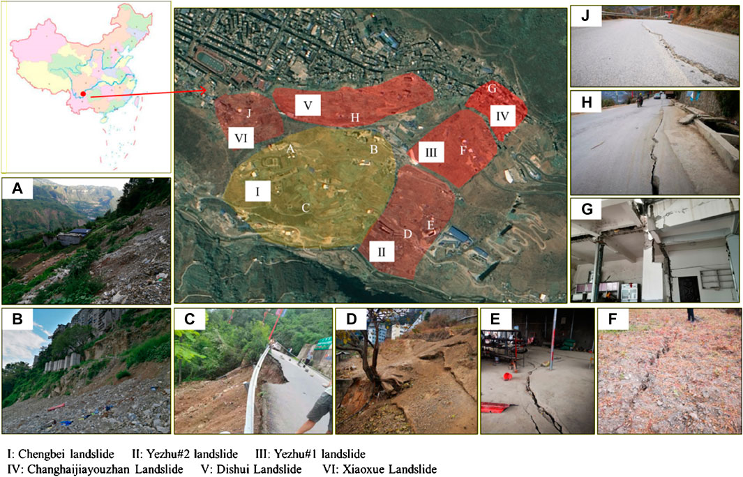
FIGURE 1. Case study region in the Tianchi village, Jinyang County, Liangshan Yi Autonomous Prefecture.

3.2 Dataset summary

According to Figure 1, a total of 19 web-based global positioning system (GPS) points are configured to monitor the slope deformation for all six landslides in real-time. The displacement time series depicting the slope deformation process are measured on a daily basis, and the measurement unit is millimeters. The data collection process was initiated on 11 Mar 2017, and we collected daily displacement data until 24 Nov 2019, for the analysis. The raw displacement data were measured in three separate directions, including the X, Y, and Z directions. In this study, the prediction models are separately developed in each direction to extract useful features in a certain direction.

4 Experimental results

To predict the future displacement following the proposed approach, autocorrelation analysis is first performed. The autocorrelation analysis computes the ACF and PACF (see Eqs 2, 3) and computes the correlation between the current displacement and the average historic displacements. As illustrated in Figure 2, the ACFs and PACFs for 15 lags are computed.

FIGURE 2

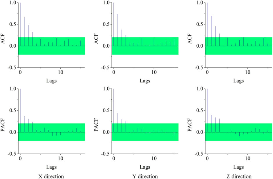
FIGURE 2. Autocorrelation analysis for the displacement series in each direction.

As shown in Figure 2, the ACFs and PACFs for GPS point #5 in three directions are visualized as an example. Here, all the lag-zero ACFs or PACFs that measure the autocorrelation between the displacements versus themselves are equal to 1, as they are completely identical. The green region denotes the threshold of significance if an ACF or PACF is significantly nonzero. The thresholds are computed based on the Ljung–Box statistics, and those outside of the threshold are considered statistically significant. In each direction, it is evident that the first three historic lags (i.e., t-1. t -2, and t -3) are significantly above zero and thus are considered as input for the prediction model.

Figure 3 shows the nonlinear relationship between the embedded dimension versus the percentage of FNN during data reconstruction. Here, we examined a total of 25 possible dimensions and correspondingly computed the percentage of FNN. The turning points (m points) denote the optimal choice for selecting the appropriate embedded dimensions. Thus, 18 embedded dimensions are suitable for displacements in the X direction, and 15 dimensions are suitable for displacements in the Y direction. In total, 20 dimensions are appropriate for the embedded dimensions in the Z direction. Integrated with the results of ACFs and PACFs, the summary of the data reconstruction parameters in each direction for GPS point #5 are summarized in Table 1. Then, the Lyapunov exponents for the reconstructed series are shown in Figure 4.

FIGURE 3

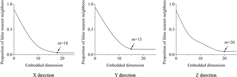
FIGURE 3. Size of the embedded dimension with respect to the percentage of FNN.

TABLE 1

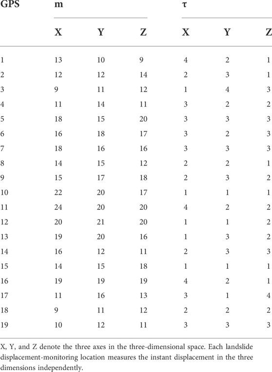
TABLE 1. Summary of the data reconstruction parameters.

FIGURE 4

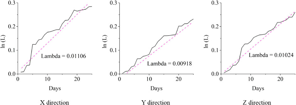
FIGURE 4. Lyapunov exponents in three directions.

Figure 4 illustrates the Lyapunov exponents for the embedded displacement time series for GPS #5 in all three directions. Here, Figure 4 shows the curve between the temporal domain (days) and ln(L), and the solution of the Lyapunov exponent is computed by the slope coefficient. Thus, the X, Y, and Z directions have Lyapunov exponents of 0.01106, 0.00918, and 0.01024, respectively. The values of the Lyapunov exponents (i.e., lambda) for GPS point #5 are all positive, which indicates that all the reconstructed displacement series are chaotic. For all 19 GPS points, the Lyapunov exponents are summarized in Table 2.

TABLE 2

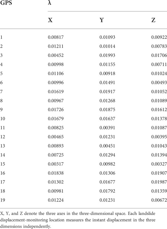
TABLE 2. Summary of the Lyapunov exponents for all GPS points.

After confirming the chaotic characteristics of the displacement series in all three directions, the LSTM networks are trained and tested for all GPS points. Following the training strategy described in Section 2.5, the prediction performance on the test dataset is obtained. Figure 5 displays the distribution of errors between the predicted displacement and measured displacement in all three directions. Additionally, the error between the merged measured displacement versus the merged predicted displacement is also computed. A summary of the MAE and RMSE (see Section 2.7) is also presented in Table 3.

FIGURE 5

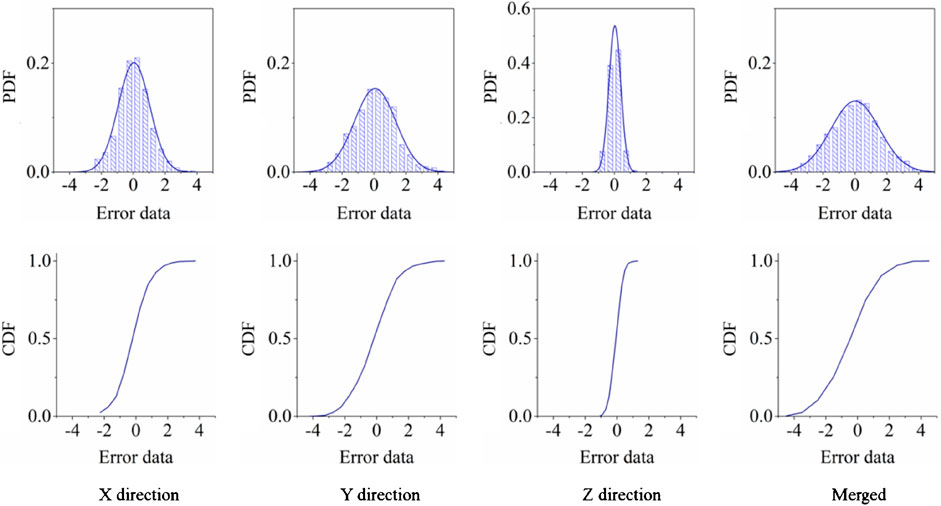
FIGURE 5. Error analysis in three directions and the merged outcome.

TABLE 3

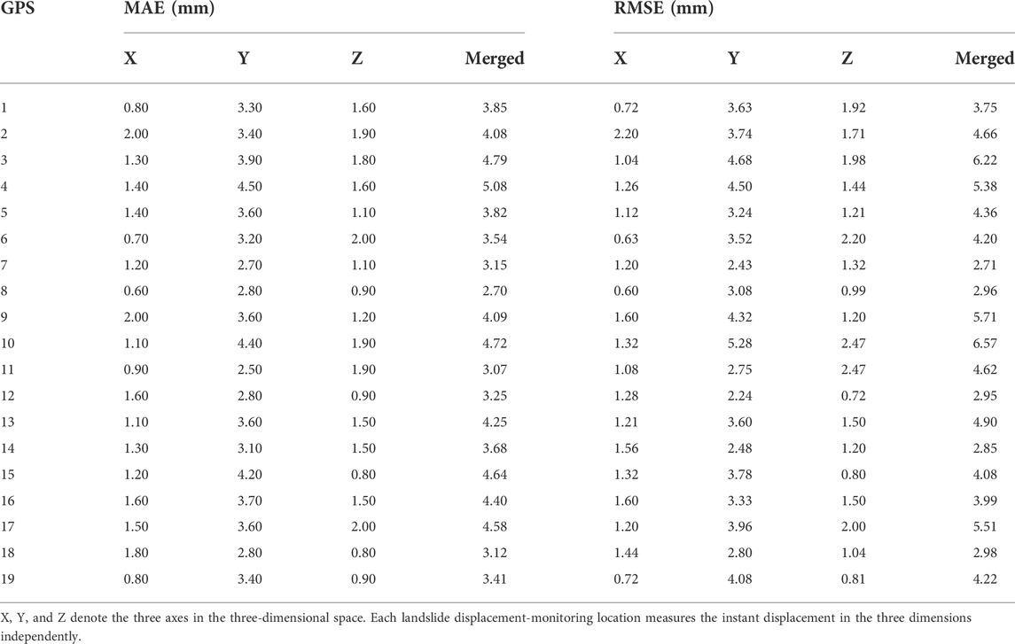
TABLE 3. Summary of the prediction performance by robust LSTM for all GPS points.

From Figure 5, it can be observed that the majority of the errors in GPS point #5 between the measured daily displacement and predicted daily displacement follow a Gaussian distribution with a mean close to zero and a certain level of variance depending on the displacement direction. The first row of pictures depicts the probability density distribution (PDF) for the error distribution. Meanwhile, the cumulative density functions (CDFs) of all errors are displayed in the second row. According to both rows of pictures, the region close to zero has high probability densities, while the distribution of prediction error is symmetric. A summary of the MAE and RMSE (see Section 2.7) is also presented in Table 3.

Table 3 presents the performance evaluation for all GPS points measured displacement. The DNN, DBN, and conventional LSTM are also tested for comparative performance analysis, and the results are presented in Table 4. The proposed robust LSTM trained with pseudo-Huber loss provides the best prediction performance among all algorithms tested with the smallest MAE and RMSE. Thus, the validity of using the proposed approach in the time-series displacement prediction is confirmed.

TABLE 4

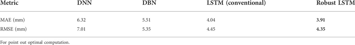
TABLE 4. Summary of the prediction performance for the algorithms tested.

5 Conclusion

In this research, the displacement prediction performance of a robust LSTM network and other machine learning algorithms is evaluated. The proposed framework contains a data reconstruction step for capturing the chaotic characteristics of the time-series displacements. Meanwhile, the LSTM network has been adopted as the prediction algorithm and is integrated with the pseudo-Huber loss to prevent impact from a few outliers.

The efficiency of the proposed framework has been validated by testing the field displacement dataset in our case study area. The computational results demonstrate that the proposed framework outperforms the conventional LSTM network as well as other machine learning algorithms in terms of all performance evaluation metrics. This study has also revealed that the pseudo-Huber loss is capable of providing improved performance in handling time-series displacement datasets.

The proposed approach can benefit on-site landslide hazard prevention in multiple ways. For instance, the pretrained algorithm can be installed in the chip of a GPS monitoring instrument for real-time prediction. Once the prediction errors surpass the statistical threshold, it triggers the alarm for faster displacement which usually caused casualties and property loss. In addition, it can be incorporated with other sources of information such as images or vibration to produce comprehensive landslide deformation monitoring, respectively.

Data availability statement

The original contributions presented in the study are included in the article/supplementary material; further inquiries can be directed to the corresponding author.

Author contributions

YX: conceptualized the study, contributed to the study methodology, and wrote the original draft. NJ: contributed to the study methodology, data curation, and investigation. CH: contributed to software and formal analysis. ZX: contributed to investigation. ZM: contributed to data analysis and investigation.

Funding

The study was financially supported by the State Key Laboratory of Geohazard Prevention and Geoenvironment Protection Independent Research Project (SKLGP2020Z006) and Sichuan Science and Technology Program (No. 2022YFG0183).

Conflict of interest

The authors declare that the research was conducted in the absence of any commercial or financial relationships that could be construed as a potential conflict of interest.

Publisher’s note

All claims expressed in this article are solely those of the authors and do not necessarily represent those of their affiliated organizations, or those of the publisher, the editors, and the reviewers. Any product that may be evaluated in this article, or claim that may be made by its manufacturer, is not guaranteed or endorsed by the publisher.

References

Aggarwal, A., Alshehri, M., Kumar, M., Alfarraj, O., Sharma, P., and Pardasani, K. R. (2020). Landslide data analysis using various time-series forecasting models. Comput. Electr. Eng. 88, 106858. doi:10.1016/j.compeleceng.2020.106858

CrossRef Full Text | Google Scholar

Arize, D., and Rios, T. N. (2019). “A comparison study on time series forecasting given smart grid load uncertainties,” in 2019 8th brazilian conference on intelligent systems (BRACIS), Salvador, Brazil, 15-18 October 2019(IEEE), 257–262.

CrossRef Full Text | Google Scholar

Fan, X., Scaringi, G., Korup, O., West, A. J., van Westen, C. J., Tanyas, H., et al. (2019). Earthquake-induced chains of geologic hazards: patterns, mechanisms, and impacts. Rev. Geophys. 57 (2), 421–503. doi:10.1029/2018rg000626

CrossRef Full Text | Google Scholar

Fan, Z., and Cai, J. (2021). Effects of unidirectional in situ stress on crack propagation of a jointed rock mass subjected to stress wave. Shock Vib. 2021, 5529540. doi:10.1155/2021/5529540

CrossRef Full Text | Google Scholar

Fan, Z., Zhang, J., Xu, H., and Wang, X. (2022). Transmission and application of a P-wave across joints based on a modified g-λ model. Int. J. Rock Mech. Min. Sci. 150, 104991. doi:10.1016/j.ijrmms.2021.104991

CrossRef Full Text | Google Scholar

Fischer, T., and Krauss, C. (2018). Deep learning with long short-term memory networks for financial market predictions. Eur. J. Operational Res. 270 (2), 654–669. doi:10.1016/j.ejor.2017.11.054

CrossRef Full Text | Google Scholar

Herrera, G., Fernández-Merodo, J. A., Mulas, J., Pastor, M., Luzi, G., and Monserrat, O. (2009). A landslide forecasting model using ground based SAR data: the Portalet case study. Eng. Geol. 105 (3-4), 220–230. doi:10.1016/j.enggeo.2009.02.009

CrossRef Full Text | Google Scholar

Hochreiter, S., and Schmidhuber, J. (1997). Long short-term memory. Neural Comput. 9 (8), 1735–1780. doi:10.1162/neco.1997.9.8.1735

PubMed Abstract | CrossRef Full Text | Google Scholar

Hungr, O. (1995). A model for the runout analysis of rapid flow slides, debris flows, and avalanches. Can. Geotech. J. 32 (4), 610–623. doi:10.1139/t95-063

CrossRef Full Text | Google Scholar

Li, D. Y., Sun, Y. Q., Yin, K. L., Miao, F. S., Glade, T., and Leo, C. (2019). Displacement characteristics and prediction of baishuihe landslide in the three Gorges reservoir. J. Mt. Sci. 16 (9), 2203–2214. doi:10.1007/s11629-019-5470-3

CrossRef Full Text | Google Scholar

Li, H., Deng, J., Feng, P., Pu, C., Arachchige, D., and Cheng, Q. (2021b). Short-term nacelle orientation forecasting using bilinear transformation and ICEEMDAN framework. Front. Energy Res. 9, 780928. doi:10.3389/fenrg.2021.780928

CrossRef Full Text | Google Scholar

Li, H., Deng, J., Yuan, S., Feng, P., and Arachchige, D. (2021a). Monitoring and identifying wind turbine generator bearing faults using deep belief network and EWMA control charts. Front. Energy Res. 9, 799039. doi:10.3389/fenrg.2021.799039

CrossRef Full Text | Google Scholar

Li, H., He, Y., Xu, Q., Deng, j., Li, W., and Wei, Y. (2022). Detection and segmentation of loess landslides via satellite images: a two-phase framework. Landslides 19, 673–686. doi:10.1007/s10346-021-01789-0

CrossRef Full Text | Google Scholar

Li, H. (2022a). SCADA data based wind power interval prediction using LUBE-based deep residual networks. Front. Energy Res. 10, 920837. doi:10.3389/fenrg.2022.920837

CrossRef Full Text | Google Scholar

Li, H. (2022b). Short-term wind power prediction via spatial temporal analysis and deep residual networks. Front. Energy Res. 10, 920407. doi:10.3389/fenrg.2022.920407

CrossRef Full Text | Google Scholar

Li, H., Xu, Q., He, Y., and Deng, J. (2018). Prediction of landslide displacement with an ensemble-based extreme learning machine and copula models. Landslides 15 (10), 2047–2059. doi:10.1007/s10346-018-1020-2

CrossRef Full Text | Google Scholar

Li, H., Xu, Q., He, Y., Fan, X., and Li, S. (2020). Modeling and predicting reservoir landslide displacement with deep belief network and EWMA control charts: a case study in three Gorges Reservoir. Landslides 17 (3), 693–707. doi:10.1007/s10346-019-01312-6

CrossRef Full Text | Google Scholar

Lian, C., Zeng, Z., Yao, W., and Tang, H. (2013). Displacement prediction model of landslide based on a modified ensemble empirical mode decomposition and extreme learning machine. Nat. Hazards (Dordr). 66 (2), 759–771. doi:10.1007/s11069-012-0517-6

CrossRef Full Text | Google Scholar

Miao, T., Liu, Z., Niu, Y., and Ma, C. (2001). A sliding block model for the runout prediction of high-speed landslides. Can. Geotech. J. 38 (2), 217–226. doi:10.1139/t00-092

CrossRef Full Text | Google Scholar

Ouyang, T., Huang, H., He, Y., and Tang, Z. (2020). Chaotic wind power time series prediction via switching data-driven modes. Renew. Energy 145, 270–281. doi:10.1016/j.renene.2019.06.047

CrossRef Full Text | Google Scholar

Pradhan, B., and Lee, S. (2010). Regional landslide susceptibility analysis using back-propagation neural network model at Cameron Highland, Malaysia. Landslides 7 (1), 13–30. doi:10.1007/s10346-009-0183-2

CrossRef Full Text | Google Scholar

Saito, M. (1965). “Forecasting the time of occurrence of a slope failure,” in Proceedings of the sixth international conference on soil mechanics and foundation engineering, Montreal, Canada, September 1965, 537–541.

Google Scholar

Tang, Y., Deng, J., Zang, C., and Wu, Q. (2022). Chaotic modeling of stream nitrate concentration and transportation via IFPA-ESN and turning point Analyses. Front. Environ. Sci. 10, 855694. doi:10.3389/fenvs.2022.855694

CrossRef Full Text | Google Scholar

Wolf, A., Swift, J. B., Swinney, H. L., and Vastano, J. A. (1985). Determining Lyapunov exponents from a time series. Phys. D. Nonlinear Phenom. 16 (3), 285–317. doi:10.1016/0167-2789(85)90011-9

CrossRef Full Text | Google Scholar

Xie, P., Zhou, A., and Chai, B. (2019). The application of long short-term memory (LSTM) method on displacement prediction of multifactor-induced landslides. IEEE Access 7, 54305–54311. doi:10.1109/access.2019.2912419

CrossRef Full Text | Google Scholar

Xing, Y., Yue, J., Chen, C., Qin, Y., and Hu, J. (2020). A hybrid prediction model of landslide displacement with risk-averse adaptation. Comput. Geosciences 141, 104527. doi:10.1016/j.cageo.2020.104527

CrossRef Full Text | Google Scholar

Zhou, J., Wei, J., Yang, T., Zhang, P., Liu, F., and Chen, J. (2021). Seepage channel development in the crown pillar: insights from induced microseismicity. Int. J. Rock Mech. Min. Sci. 145, 104851. doi:10.1016/j.ijrmms.2021.104851

CrossRef Full Text | Google Scholar