 Edmund K. M. Chang
 Yutong Pan2,3
94% of researchers rate our articles as excellent or good
Learn more about the work of our research integrity team to safeguard the quality of each article we publish.
Find out more
ORIGINAL RESEARCH article
Front. Earth Sci., 17 October 2022
Sec. Atmospheric Science
Volume 10 - 2022 | https://doi.org/10.3389/feart.2022.963779
Extratropical cyclones give rise to most of the high impact weather in the mid-to high-latitudes during the cool seasons, including heavy precipitation and strong winds. Thus it is important for stakeholders to be informed of approaching periods of increased or decreased cyclone activity. While individual cyclone tracks can be predicted out to about a week or so, from week 2 on, statistics summarizing cyclone activity, or storminess, are more useful. Storminess can be defined based on Lagrangian cyclone tracking or by Eulerian variance statistics. The outlook includes a combination of both methods. Lagrangian cyclone tracks provide information about where cyclones pass through and are more intuitive to users, while Eulerian variance statistics have been shown to be highly correlated with cyclone-related weather and are expected to be more predictable given that they are not as noisy. In this paper, we evaluate a storminess outlook tool developed based on dynamical model forecasts in the week-2 and weeks 3-4 time ranges. The outlook uses two 6-hourly subseasonal ensemble forecasts–the Global Ensemble Forecast System version 12 (GEFSv12), and the coupled Climate Forecast System version 2 (CFSv2). Hindcasts and operational forecasts from 1999–2016 are used to assess the prediction skill. Our results show that the GEFSv12 and CFSv2 combined ensemble has higher skill than either individual ensemble. The combined ensemble shows some skill in predicting cyclone amplitude and frequency out to weeks 3-4, with highest skill in winter, and lowest skill in summer. Models also show some skill in predicting the statistics of deep cyclones for week 2. The prediction skills for an Eulerian sea level pressure variance storminess metric is significantly higher than those for Lagrangian track statistics. Our results also show that GEFSv12 performs better than its predecessor GEFSv11. Correlations between the storminess indices and surface weather, including precipitation and high winds, are examined. A publicly accessible web page has been developed to display the subseasonal predictions in real time. The web page also contains information on climatology and forecast verification to enable users to make more informed use of the outlook.
Extratropical cyclones and their fronts are responsible for much of the high impact and extreme weather over the mid-latitudes. On the global scale, Pfahl and Wernli (2012) showed that over most extratropical regions, precipitation extremes frequently coincide with occurrences of cyclones. Over the U.S., almost 80% of the extreme precipitation events are caused by extratropical cyclones, not only during the cool season, but throughout the year (Kunkel et al., 2012).
Extratropical cyclones also generate high wind events which cause not only property damages but also fatalities (e.g., Ashley and Black, 2008). Sustained high winds associated with extratropical cyclones can also lead to storm surges that give rise to coastal flooding (e.g., Colle et al., 2008; Salmun et al., 2011). On top of these, during winter, extreme cold events are associated with passages of cyclones and anticyclones that develop and propagate along the storm track (e.g., Kocin et al., 1988), and lack of cyclone events in summer can lead to enhanced heat waves (Chang et al., 2016). All these adverse weather events have caused significant economic losses and fatalities in the past (e.g., Berko et al., 2014). Thus accurate predictions of the possible occurrences of these events are needed to enable policy makers and emergency management to have sufficient lead time to plan for mitigation and adaptation.
Two types of metrics have been used to quantify storminess: Lagrangian cyclone track statistics and Eulerian variance statistics. In the first type, cyclones can be tracked using automated cyclone tracking algorithms (for example Serreze, 1995; Hodges, 1994), by finding minima in gridded sea level pressure (SLP) data, and connecting together closest centers at consecutive time steps to form tracks. After the tracks have been obtained, summary statistics such as track frequency and average storm amplitude (e.g., in terms of the central SLP) can be generated. The advantage of this type of statistics is that it is intuitive to users–high impact weather events are frequently located at specific locations around cyclone centers (e.g. Lackmann, 2011), thus visualizing the predicted cyclone tracks provide users with information about which areas will be impacted by the expected weather associated with the cyclones.
The development and propagation of individual cyclones can generally be predicted out to about one week (e.g., Froude et al., 2007; Charles and Colle, 2009; Froude, 2010). However, to date it is not clear how well Lagrangian cyclone track statistics can be predicted in the subseasonal time scale. Lukens and Berbery (2019) assessed weeks 3-4 cyclone track predictions near North America by the coupled Climate Forecast System version 2 (CFSv2; Saha et al., 2014) in winter. They found that after bias correction, the model climatology can well depict observed features. However, the root-mean-squared (RMS) errors in both predicted cyclone frequency and amplitude are close to or exceed the standard deviation of variability over most regions, suggesting little or no skill. Additionally, Lukens and Berbery (2019) compared statistics derived from a single forecast, instead of an ensemble mean forecast, to observed statistics. As numerous studies have shown in the past (e.g., Atger, 1999; Zhu, 2005), in the extended time range, ensemble mean forecasts generally outperform single member deterministic forecasts due to the removal or reduction in the ensemble mean of the noise related to the chaotic behavior of the atmosphere. Thus one can hypothesize that ensemble mean track statistics forecasts may be skillful for a sufficiently large ensemble in the subseasonal time scale. Note that a recent study (Zhang et al., 2021) suggested that certain statistics of wave breaking related to Lagrangian cyclone tracks may be predictable in the seasonal time scale using large ensembles.
The second type of metrics to quantify storminess is Eulerian variance statistics. Given that cyclones are low pressure systems, passages of cyclones over any location give rise to rapid pressure changes. Thus 12- or 24-h pressure tendencies at a fixed location have been frequently used to quantify cyclone activity (e.g., Alexander et al., 2005; Feser et al., 2015). One simple Eulerian storminess metric is variance computed using the 24-h difference filter which highlights eddy activity with periods between 1.2 and 6 days (Wallace et al., 1988), as follows:
In (Eq. 1), ECApp denotes Extratropical Cyclone Activity (ECA) derived from 24-h filtered SLP variance. The overbar denotes averaging over a time period (e.g., one week, two weeks, or one month). This statistic can be computed at every grid point or location using the time series of station observations, analysis, or forecast SLP data. As shown in many previous studies (Wallace et al., 1988; Chang, 2013; see also discussion below), this metric highlights the Pacific and Atlantic storm tracks, along with the extension of the storm track from the Pacific towards the Atlantic across North America, and its climatological distribution clearly exhibits significant resemblance to the Lagrangian track statistics (see, e.g., Supplementary Figures S1, S24). In addition, previous studies have shown that the variability of this metric is highly correlated with variations in precipitation (Chang, 2013; Chang et al., 2015; Zheng et al., 2018; Yau and Chang, 2020) and frequency of extreme events including high winds, heavy precipitation, and extremely cold temperatures (Ma and Chang, 2017; Yau and Chang, 2020). Note that while Eulerian and Lagrangian storminess exhibit quite a bit of similarities, there are differences between them. For example, quasi-stationary cyclones contribute to Lagrangian track statistics and do not contribute much to Eulerian statistics. In addition, variations in Eulerian statistics generally reflect a combination of changes in cyclone frequency and amplitude and cannot be decomposed to quantify variations in frequency or amplitude, while Lagrangian statistics can provide additional information such as cyclone genesis and lysis locations and frequency.
Is this Eulerian storminess metric predictable by the current generation of climate prediction models? Previous studies (e.g. Grise et al., 2013; Guo et al., 2017) have shown that Eulerian storminess metrics are generally not as noisy as Lagrangian metrics, suggesting that they may be more predictable. Yang et al. (2015) showed that seasonal variations of this metric associated with the El Nino-Southern Oscillation (ENSO) can be predicted out to 9 months by the Geophysical Fluid Dynamics Laboratory (GFDL) climate prediction model. For the subseasonal timescale, Zheng et al. (2019) and Zheng et al. (2021) demonstrated that the Subseasonal-to-Seasonal (S2S; Vitart et al., 2017) and the Subseasonal Experiment (SubX; Pegion, 2019) ensembles, including CFSv2 and the Global Ensemble Forecast System version 11 (GEFSv11; Zhou et al., 2017), exhibit significant skills in predicting this metric out to week 4 in winter. Previous studies have shown that in the subseasonal to seasonal timescale, extratropical storminess is modulated by the large-scale, low frequency variability of the climate system including ENSO (Straus and Shukla, 1997; Eichler and Higgins, 2006); the Madden-Julian Oscillation (MJO; Deng and Jiang, 2011; Guo et al., 2017; Zheng et al., 2018); polar vortex variability (Baldwin and Dunkerton, 2001; Walter and Graf, 2005); and the Quasi-Biennial Oscillation (QBO; Wang et al., 2018). Zheng et al. (2019) and Zheng et al. (2021) showed that the weeks 3-4 prediction skill exhibited by the models is largely consistent with the ability of the models to predict the impacts of ENSO and polar vortex variability on mid-latitude storminess.
In this study, we will evaluate how well a combined ensemble made up of CFSv2 and a newer version of GEFS (v12; Guan et al., 2022) does in predicting the subseasonal variations of extratropical storminess, for both Eulerian and Lagrangian storminess metrics. We will address 3 main questions: 1) Whether model ensembles can predict Lagrangian storminess as well as Eulerian statistics; 2) How well models can predict storminess in seasons other than winter; and 3) Whether GEFSv12 predictions exhibit any improvement over those of GEFSv11.
An extratropical storminess outlook tool based on both types of metrics has been developed and will be described. We will also discuss the sensitivity of model performance to choices of parameters, including radius for accumulating cyclone track statistics, cyclone depth cutoff, and bias correction.
As discussed above, much of the interests in storminess prediction arise from the close relationship between the variations in storminess and those in weather, such as precipitation and strong winds. Yau and Chang (2020) developed an index (CORMAX, see discussions in CORMAX between Storm Track Metrics and Weather Section below) to quantify the strength of this relationship, and we will use this index to examine how well each of the different storminess metrics examined in this study relates to the variability of the weather elements.
The model data for the subseasonal prediction are taken from the 16-day and 35-day GEFSv12 and 45-day CFSv2 model outputs available at a 6-h interval. The data consist of both hindcasts and operational forecasts. The model data are on a 0.5° × 0.5° grid in GEFSv12 and a 1° × 1° grid in CFSv2. We have focused on these two model ensembles because they are the only models that provide 6-hourly data needed for cyclone tracking. The data are interpolated onto a 2.5° × 2.5° grid for computational efficiency, while allowing a reasonable representation of cyclone activity which has decorrelation length scales that are much larger than 250 km.
The GEFSv12 16-day hindcasts are initialized at 00Z daily with five members. The GEFSv12 35-day hindcasts are also initialized at 00Z but on every Wednesday with 11 members. Therefore, the 35-day hindcasts have more ensemble members than the 16-day hindcasts, but with less frequent initializations. The 45-day CFSv2 hindcasts are initialized 4 times daily at 00Z, 06Z, 12Z and 18Z with a total of four members every day. In this study, data from 1999–2016, the same period examined by Zheng et al. (2021), are used to assess the hindcasts. We have also examined daily-mean data from the GEFSv11 35-day hindcasts for the same period in comparison with GEFSv12 hindcasts.
For operational forecasts, both GEFSv12 and CFSv2 have many more ensemble members than their hindcasts. The GEFSv12 16-day forecasts are initialized at 00Z, 06Z, 12Z, and 18Z, each with 31 members and a daily total of 124 (31 × 4) members. The GEFSv12 35-day forecasts are only available with the 00Z initialization and thus have 31 members daily. Like the GEFSv12 16-day forecasts, the CFSv2 45-day forecasts are also initialized 4 times daily at 00Z, 06Z, 12Z, and 18Z. However, for each initialization time, there are four ensemble members and a daily total of 16 members. Operational forecast data are used to generate the near real time subseasonal outlook and posted online on the web page described in Real Time Outlook Tool Web Page Section.
To validate and assess the model forecasts, reanalysis data are used, which are taken from the Climate Forecast System Reanalysis (CFSR; Saha et al., 2010) with a 6-h interval and a half degree resolution. The variables used include SLP, precipitation, and 10-m wind. We have also used reanalysis data from ERA5 (Hersbach et al., 2020) to assess the model hindcasts. Assessment based on ERA5 data will be shown in this paper. Results based on CFSR are similar and will be displayed on the web page described below.
To relate the storminess indices to precipitation, monthly-mean precipitation data from the Global Precipitation Climatology Project (GPCP; Adler et al., 2018) from 1979 to 2018 on a 2.5° × 2.5° grid are used.
To relate the storminess indices to high wind conditions, following Yau and Chang (2020), we used a high wind index defined as the 95th-percentile 6-hrly 10-m wind speed for each month at each grid point derived from reanalysis data. This is similar to the high wind index used by Paciorek et al. (2002). As discussed in Paciorek et al. (2002), since reanalysis data are not real observations, this index is used not to represent the actual observed high winds, but as an indicator of when high wind conditions are expected. We have also examined an alternative high wind index defined by the frequency of 10-m wind speed exceeding gale force (>17.2 ms−1) in a month at each grid point.
In this study, we have examined both Lagrangian cyclone tracking statistics that are derived from identifying and tracking cyclones, as well as Eulerian variance statistics derived based on the SLP time series at each grid box.
Cyclones can be defined in many ways (see Neu et al., 2013), including minima in SLP, minima in SLP anomalies (deviations from a large-scale background field), surface vorticity maxima, 850 hPa vorticity maxima, and so on. In this study, cyclone centers are defined by the minima in the total SLP field, mainly because this is the definition that forecasters are most familiar with–see, for example, the surface analyses produced by the Weather Prediction Center.
Cyclone detection and tracking are based on the algorithm developed by Serreze (1995) with the following criteria using 6-h SLP data over the Northern Hemisphere on a 2.5° × 2.5° grid: 1) Storm center SLP ≤1000 hPa, 2) Storm center SLP at least 1 hPa lower than the neighboring grid points, and 3) Maximum distance a storm can travel is 800 km/6 h.
We have also tested the impact of removing condition 1 - that is, including all identified cyclone centers regardless of central pressure for deriving track statistics. The results of the sensitivity test will be discussed in Cyclone Minimum Pressure Cutoff Value Section.
After the cyclone centers and tracks have been identified, statistics such as track frequency (or density) and amplitude (or intensity) can be computed. Since the cyclone related significant weather, including precipitation and high winds, impact a region out to hundreds of kms away from the cyclone center (Chang and Song, 2006; Field and Wood, 2007; Bengtsson et al., 2009), many studies have accumulated cyclone statistics within a radius of ∼500 km of the center of each grid box (e.g. Sinclair, 1997; Grise et al., 2013; Guo et al., 2017; Yau and Chang, 2020). After testing accumulating statistics within radii of 250 and 500 km, we decided to use 500 km as the radius for accumulating cyclone statistics. The results of the sensitivity test will be discussed in Radius for Accumulating Track Statistics Section.
Following Yau and Chang (2020), cyclone track frequency (or density) is defined as the number of cyclone tracks that pass within 500 km of the center of each grid box within the forecast period. Each cyclone is only counted once regardless of how long it stays within 500 km of a grid box. Track amplitude (or intensity) is the average of the amplitude of all cyclones that pass within 500 km of the grid box during the forecast period. For a cyclone that stays within 500 km of the center of the grid box for multiple time steps, the amplitude that is accumulated is the maximum amplitude (lowest central SLP) the cyclone attains during these time steps. To account for fast moving cyclones that jump over multiple grid boxes within a single 6-h time period, the cyclone track is linearly interpolated into hourly time steps before the cyclone statistics are computed. Cyclone statistics are accumulated on a 2.5° × 2.5° grid. The seasonal climatology for track frequency and amplitude based on ERA5 data, as well as the model forecast biases, are displayed in the Supplementary Figures S1–S23.
The Eulerian storminess statistic examined is the 24-h difference filtered SLP variance statistic (ECApp) defined by Eq. 1 above. This metric highlights synoptic timescale (1.2–6 days) SLP variability. ECApp can be computed at each grid point using (Eq. 1) based on the reanalysis or model forecast/hindcast time series of SLP at that grid point. The statistic is averaged over 1 week for week 2 forecasts, and 2 weeks for weeks 3-4 forecasts. The seasonal climatology and model forecast biases for ECApp are displayed in the Supplementary Figures S24–S28.
Hindcasts are assessed using the Anomaly Correlation Coefficient (ACC) between storminess indices derived from model hindcasts and reanalysis data at each grid point. As discussed above, the 35-day GEFSv12 hindcasts are initialized every 7 days (weekly at 00Z on Wednesdays) and provide an 11-member ensemble for each hindcast. Hence we also only sample CFSv2 hindcasts for the same initialization dates. Since CFSv2 hindcasts are initialized every 6 h, but only provide one-member for each initialization, to form a CFSv2 ensemble, a lagged-ensemble strategy has to be employed. Zheng et al. (2021) showed that for SLP variance statistics, the weeks 3-4 hindcast ACC scores for CFSv2 increase with the number of lagged members up to over 10 members. Here, we use a 12-member lagged ensemble, hence including hindcasts that are initialized up to nearly 3 days prior to the initialization time (00Z every Wednesday). Hence the combined GEFSv12/CFSv2 ensemble has 23 members. Hindcast data from 1999 to 2016 have been assessed—a total of 18 years of hindcasts.
Anomalies are defined by subtracting the model ensemble-mean hindcast storminess climatology from each model ensemble-mean storminess hindcasts. Model climatology is defined daily. Since the initialization dates are all on Wednesday, with 18 years of data, each calendar day has only 2-3 initializations over the entire period. Hence the hindcast climatology is smoothed by including all hindcasts within 20 days prior to or following the initialization date, thus averaging over about 100 hindcast cases to produce the climatology for each day. Reanalysis climatology is defined the same way and thus represents a 41-day running mean, except that there is no ensemble-mean for reanalysis storminess.
Previous studies have only examined storminess forecasts for winter. In this study, the seasonal variation in the ability of models to predict storminess is assessed. For assessment purposes, model hindcasts are grouped into 2-month periods: Fall (October/November or ON); early winter (December/January or DJ); late winter (February/March or FM); spring (April/May or AM); early summer (June/July or JJ); and late summer (August/September or AS). The hindcast ACC for each period is computed using hindcasts that have at least half of their validation period falling within the 2-month period.
Given that model hindcasts have biases (Supplementary Figures S1–S28 in the Supplementary Material), defining hindcast anomalies by subtracting off model climatology corresponds to bias correction. In Bias Correction Section we will examine how this simple bias correction impacts model hindcast skill.
For each 2-month period, there are about 150 hindcasts over the 18 years. Since we only consider hindcasts that are initialized one week apart, all week 2 hindcasts are non-overlapping. Since week-to-week storm track variations at a grid box are not significantly correlated, these 150 hindcasts can be considered independent in time. For 150 independent data pairs, an ACC value above 0.16 is statistically significant at the 95% level. For weeks 3-4 hindcasts, consecutive hindcasts overlap for one week, and hence cannot be considered independent. For each 2-month period, there are about 75 non-overlapping hindcasts which can be considered independent. With 75 data pairs, an ACC value of 0.23 is statistically significant at the 95% level.
To assess forecast skill, one should compare it to a reference “no-skill” forecast. The most commonly used no-skill forecasts are random or climatological forecasts. For both cases, the expected ACC score is 0, hence model hindcasts that are positive and statistically significantly different from 0 (see previous paragraph) can be considered to be skillful compared to both random and climatological forecasts.
Due to statistical fluctuations, even a no-skill forecast can have some grid points that are statistically significant. Hence a few isolated significant points on an ACC map may not necessarily indicate that the model predictions are skillful, while if most of the ACC values are significantly positive, the model predictions are likely skillful. This can be assessed quantitatively using a field significance test (Livezey and Chen, 1983) based on the Monte Carlo technique. Details of the field significance test can be found in the Supplementary Material (Supplementary Text S2.1).
In this study, we have assessed model skill based on the ACC score. Previous studies have assessed model skill by computing the root-mean-squared-error (RMSE). We have conducted some assessments using MSE as the skill metric and these results are briefly discussed in the Supplementary Material (Supplementary Text S2.2).
As discussed in the Introduction, extratropical cyclones are responsible for much of the sensible weather in the mid-latitudes, including precipitation and high winds. Yau and Chang (2020) quantified the statistical relationship between different storminess metrics and surface weather using a metric that estimates the maximum one-point correlation between the precipitation (or the high wind index) at each grid box and the storminess metric, and referred to that as CORMAX. Note that CORMAX is computed based on monthly mean data, since observed GPCP precipitation is only available at monthly temporal resolution prior to October 1996. We expect that weekly or bi-weekly correlations between weather and storminess metrics to be slightly lower due to the data being more noisy when averaged over shorter periods of time, but the correlation patterns should be similar.
To calculate CORMAX for precipitation at a grid box, the monthly GPCP precipitation time series at that grid box is used as the reference time series. As will be shown below, models do best in predicting both Eulerian and Lagrangian storminess metrics during winter, hence we will focus on CORMAX for winter (DJFM) in this study. Monthly data from 1979–2018, a total of 160 months of data, are used. First, the reference time series is correlated with the storminess metric, for example the monthly SLP variance metric (ECApp), at all grid points. The resulting one-point correlation map for precipitation at 38.75 °N, 121.25 °W (over California), is shown in Figure 1A. As Chang et al. (2015) showed, precipitation over California in winter is highly correlated with ECApp over eastern Pacific just offshore of the west coast of North America, with the maximum correlation reaching a value of 0.76. This value is taken to be the value for CORMAX at this grid box (38.75 °N, 121.25 °W). Note that the maximum correlation in general does not occur at the reference grid box, since the weather associated with extratropical cyclones extends hundreds of kms away from the cyclone centers. Similar one-point correlation maps can be computed using the precipitation at every grid box as the reference time series, and the maximum correlation found on each one-point correlation map in the vicinity of the reference grid box can be plotted on each grid box to form the map displaying the value of CORMAX for all grid boxes. This summary map is shown in Figure 2A for the relationship between GPCP precipitation and ECApp.
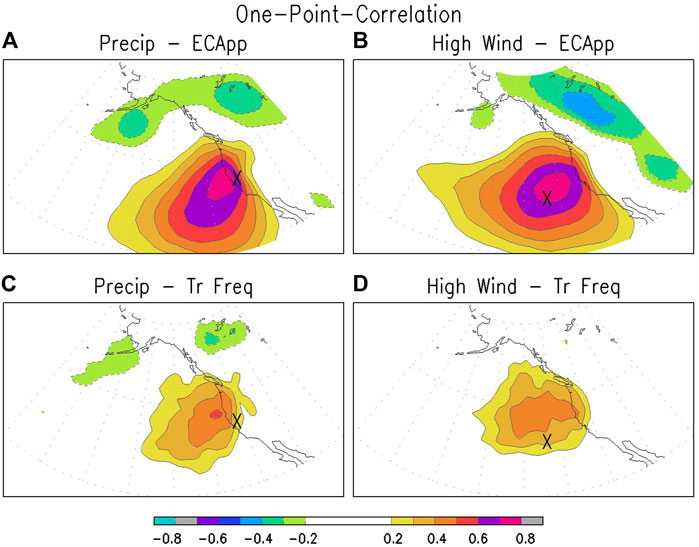
FIGURE 1. (A) One-point correlation between GPCP precipitation at 38.75 °N, 121.25 °W (marked by ‘X’) and ECApp at each grid point. (B) Similar to (A), but for the high wind index at 36.25 °N, 133.75 °W and ECApp at each grid point. (C,D) Similar to (A,B), but for cyclone track frequency instead of ECApp.
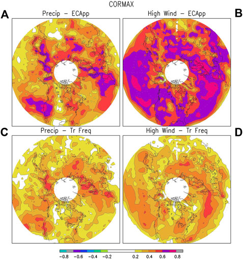
FIGURE 2. (A) CORMAX relating GPCP precipitation at each grid box to ECApp. (B) Similar to (A), but relating the high wind index at each grid box to ECApp. (C,D) Similar to (A) and (B), but for cyclone track frequency instead of ECApp.
Similar correlations can be computed based on the high wind index described in Reanalysis and Observational Data Section (the 95th percentile wind speed for each month based on ERA5 6-hrly 10-m wind data). Again, based on the monthly time series of this index at a grid-box, a one-point correlation map between this reference time series and ECApp can be computed. An example, based on the high wind index time series at 36.25 °N, 133.75 °W (over eastern Pacific), is shown in Figure 1B. The correlation between this time series and ECApp in its vicinity is quite high, with a broad area showing correlation over 0.7. The maximum value of about 0.76 is then taken to be the value for CORMAX at this grid box. Similar correlation maps can be computed for all other grid boxes, and the CORMAX value for each grid box can be found. The resultant summary map is shown in Figure 2B.
The same procedure can be repeated to relate ECApp to other weather elements, or to relate other storminess metrics (e.g. cyclone track frequency) to precipitation (Figures 1C, 2C) or other weather elements (e.g., the high wind index, Figures 1D, 2D). These will be discussed further in Correlation with Precipitation and Wind Section below.
In summary, CORMAX between a weather element (e.g., precipitation or high wind) and a storminess metric (e.g., ECApp or cyclone track frequency) summarizes how strong the correlation between the two are. The value of CORMAX at a grid point quantifies the maximum correlation between the variations in the weather element at that grid point and the variations in the storminess metric in the vicinity of that grid point. A high value of CORMAX indicates that there is high correlation between the variations of storminess and the weather element at that grid point, while a low value indicates that the correlation between the two is weak.
As discussed above, model performance in predicting storminess is assessed by computing the ACC score between model predicted and reanalysis storminess. We have examined the ACC score for the individual ensembles as well as the combined ensemble. An example is shown in Figure 3, for week 2 SLP variance in late winter (February/March). Overall, the models can predict this storminess metric with high accuracy (ACC >0.5) over extended regions over the Northern Hemisphere. Comparing the performance of the GEFSv12 and CFSv2 ensembles (Figures 3A,B), GEFSv12 performs better. The ACC for GEFSv12 is generally higher (see the number on the top right corner of each panel), except over northeastern Siberia near Alaska. We hypothesize that overall GEFSv12 performs better partly because the CFSv2 hindcast ensemble is a lagged ensemble using hindcasts initialized up to nearly 3 days old, while all GEFS ensemble members are initialized at day 0. Overall, the combined ensemble (Figure 3C) performs better than either individual ensemble, with the combined ensemble having the highest ACC scores over most regions, as well as when averaged over the northern hemisphere. This is true for all cases that we tested. From now on we will only discuss results for the combined GEFSv12/CFSv2 hindcast ensemble with 23 members.
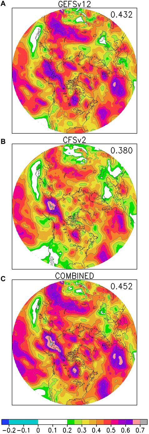
FIGURE 3 . (A) ACC scores for week 2 hindcasts of late winter (February/March) SLP variance (ECApp) by GEFSv12 ensemble; (B) Same as (A) but for CFSv2 ensemble; (C) Same as (A) but for the combined GEFSv12/CFSv2 ensemble. As discussed in the text, for week 2 hindcasts, an ACC value of 0.16 is statistically significant at the 95% level, hence all shaded areas, apart from the light blue shade for small negative correlations, are statistically significant. For this and subsequent figures, the number on the top right corner of each panel corresponds to the ACC score averaged over the western hemisphere (180 °W—0 °E; 25–70 °N).
Zheng et al. (2021) only examined model hindcasts for winter (December-January-February). Figure 4 shows how the hindcast ACC score varies as a function of the year. The highest scores are for winter–December/January and February/March (Figures 4B,C), when the ACC scores are above 0.5 over extended regions across the Northern Hemisphere, including much of the North Pacific, North Atlantic, the northern part of North America, as well as the eastern part of Asia. Model prediction skill is overall not as good as winter during the transition seasons (Figures 4A,D), with high ACC scores over more or less similar regions as in winter, but overall scores being lower by between 0.05 and 0.1. The ACC scores were lowest in summer (Figures 4E,F), with only isolated regions showing high ACC, for example over the Pacific extending into the western part of North America as well as over the northeastern part of Asia in both June/July and August/September. In summary, for week 2 hindcasts, model predictions are best in winter and worst in summer.
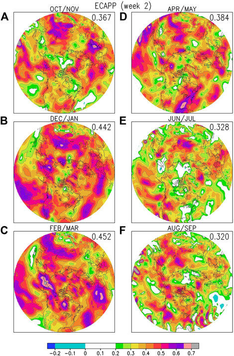
FIGURE 4. ACC scores for week 2 hindcasts of SLP variance by the combined ensemble, for (A) fall (October/November); (B) early winter (December/January); (C) late winter (February/March); (D) spring (April/May); (E) early summer (June/July); (F) late winter (August/September). An ACC value of 0.16 is statistically significant at the 95% level.
Results for weeks 3-4 hindcasts are shown in Figure 5. Model prediction skill is best in late winter (February/March, Figure 5C), when the ACC scores are relatively high over parts of the North Pacific extending towards Alaska, parts of northeastern North America, parts of the Atlantic extending towards the British Isles and Scandinavia, and part of East Asia. During early winter (December/January, Figure 5B), high scores occur over more limited regions–over the eastern Pacific extending towards North America, and over the Atlantic extending towards Europe. These results are consistent with those of Zheng et al. (2019, 2021), who showed that S2S and SubX model ensembles exhibit similar abilities to predict SLP variance during winter for weeks 3-4.
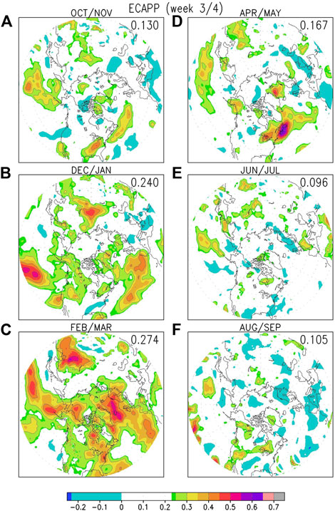
FIGURE 5. Same as Figure 4, but for weeks 3-4 hindcasts of SLP variance. For weeks 3-4 hindcasts, an ACC value of 0.23 is statistically significant at the 95% level, hence all shaded areas, apart from the light blue shade for small negative correlations, are statistically significant.
For spring (Figure 5D), models are able to predict storminess with moderate ACC scores over northeastern North America extending into the North Atlantic, western and central Pacific, and parts of east Asia. The ACC scores for fall (Figure 5A) are highest over the similar regions as for spring but are generally slightly lower. During summer (Figures 5E,F), model predictions only show isolated regions of moderate ACC scores for weeks 3–4. Overall, similar to week 2, models predict storminess best during winter and worst over summer. Not surprisingly, the ACC scores for weeks 3-4 are much lower than those for week 2. We have also examined the ACC scores for week 3 predictions alone (not shown), and the results showed that the ACC scores for weeks 3-4 combined are generally slightly higher than those for week 3 alone, probably because averaging over weeks 3 and 4 reduces noise. Hence we will combine weeks 3-4 together for the subseasonal outlook instead of splitting the two-week period into week 3 and week 4 separately.
The ACC scores for week 2 hindcast of track frequency for all cyclones are shown in Figure 6. It is clear that the ACC scores for track frequency are much lower than those for SLP variance (Figure 4), with only limited regions displaying ACC scores of >0.5. Models again show highest ACC scores for winter (Figures 6B,C), with moderate scores over much of the Pacific, parts of the continental U.S., much of the Atlantic, extending into Europe and the northern part of Eurasia. Slightly lower scores are found over the similar regions for fall (Figure 6A) and spring (Figure 6D), with more regions showing very low ACC scores (<0.2 or even negative) during summer (Figures 6E,F), suggesting that the models have limited ability to predict cyclone track frequency during summer. Over the U.S., especially over the Ohio Valley and Great Lakes region, the model hindcasts show moderate ACC scores for most of the year except during early summer (Figure 6E).
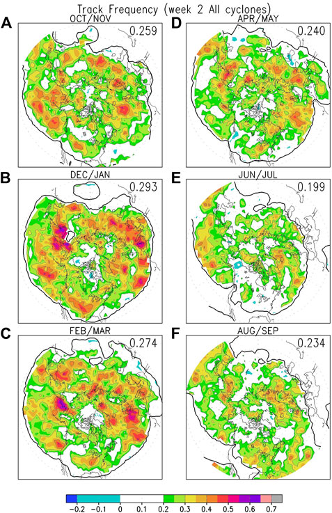
FIGURE 6. Same as Figure 4, but for week 2 hindcasts of cyclone track frequency of all cyclones. The thick solid contour corresponds to a cyclone track frequency of 0.1/week.
In Figure 7, similar scores for the model hindcasts of track amplitude (or cyclone intensity) for all cyclones are shown. The highest scores are again for winter (Figures 7B,C) over the main Pacific and Atlantic storm track regions. The ACC scores are again lower for fall and spring (Figures 7A,D), and lowest for summer (Figures 7E,F). The ability of models to predict track amplitude over North America seems to vary across the seasons, with moderate ACC scores over much of the eastern part of the U.S. in early winter (Figure 7B) and spring (Figure 7D), but rather low scores over this region during the other months.

FIGURE 7. Same as Figure 6, but for week 2 hindcasts of cyclone amplitude of all cyclones.
As discussed above, previous studies have shown that cyclone tracks may not be robust for weak cyclones (Hodges et al., 2011; Neu et al., 2013), with agreement across different tracking algorithms and data sets being more robust for moderate and strong cyclones. Hence, we also examined how well models predict cyclones with minimum SLP <1000 hPa, by removing all instances when the SLP at the cyclone center is above 1000 hPa. The results for track density are shown in Figure 8. Compared to the same statistic for all cyclones (Figure 6), when we only sample cyclones when their minimum SLP is lower than 1000 hPa, the ACC scores are slightly higher for all seasons, while the patterns are very similar.
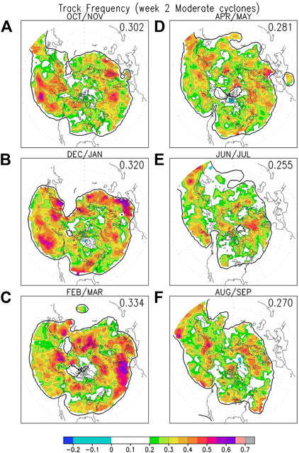
FIGURE 8. Same as Figure 6, but for week 2 hindcasts of cyclone track frequency of moderate cyclones with central SLP <1000 hPa.
However, the ACC scores for track amplitude for cyclones deeper than 1000 hPa are lower than those for all cyclones (compare Figure 9 to Figure 7). Moderate scores are found over the eastern Pacific and the Atlantic for the winter months (Figures 9B,C), and over similar regions in Fall but with lower scores (Figure 9A). During spring and summer (Figures 9D–F), models do not show appreciable skill in predicting this metric. This may be partly due to the fact that when only cyclones deeper than 1000 hPa are retained, the range of variation in cyclone intensity becomes rather narrow over most regions, except for the vicinity of the Aleutian and Icelandic low regions where cyclones can be very deep and even cyclones deeper than 1000 hPa can have amplitude spanning a large range.
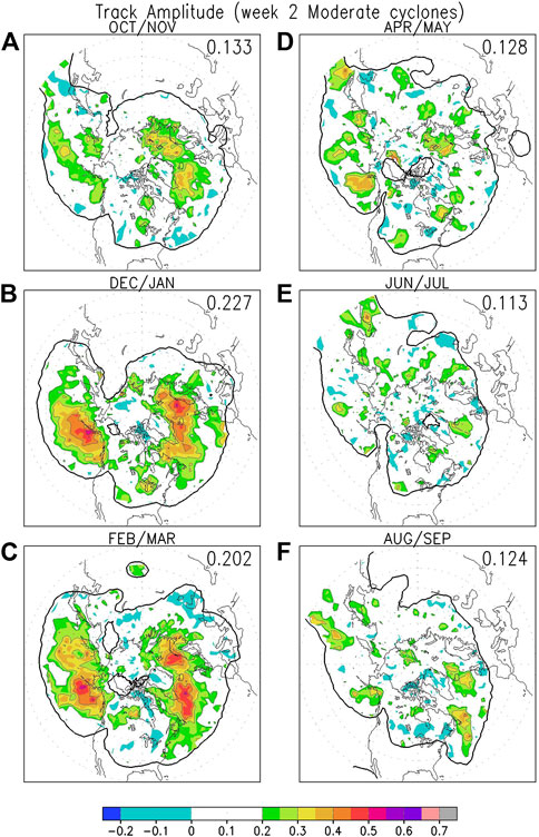
FIGURE 9. Same as Figure 8, but for week 2 hindcasts of cyclone amplitude of moderate cyclones.
We have also examined whether models can predict the statistics of deep cyclones–those with central pressure below 970 hPa. These cyclones are most frequent in winter, and are rare in the other seasons except for fall (see Supplementary Figure S21), hence we will only show evaluations for fall and winter (Figures 10A–C). Over the main regions where these cyclones frequent, the models show some ability to predict the frequency of deep cyclones, with highest ACC scores close to Alaska in the northeastern Pacific, and close to Iceland in the Atlantic. Overall, models predict these cyclones slightly better during late winter than early winter or fall.
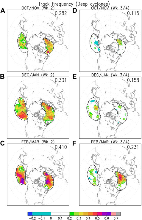
FIGURE 10. (A–C): Same as Figure 6, but for week 2 hindcasts of cyclone track frequency of deep cyclones (central SLP <970 hPa). (D–F): Same as (A–C), but for weeks 3-4 hindcasts of cyclone track frequency of deep cyclones.
Figure 11 shows how well the 23-member combined GEFSv12/CFSv2 ensemble predicts cyclone track frequency for moderate cyclones (those with central pressure below 1000 hPa) for weeks 3–4. Overall, the ability to predict track statistics for this period is quite low. Models do best for winter (Figures 11B,C), with statistically significant ACC scores over parts of eastern Pacific, and parts of the Atlantic extending from the east coast of North America towards Europe. The models seem to do slightly better during late winter than in early winter. Outside of these regions, the ACC scores are not statistically significant, and are even negative (but not significant) over some regions. The ACC scores for the other seasons are generally very low and are only statistically significant over very isolated regions. Hence our results suggest that dynamical models display limited ability to predict cyclone track statistics in the subseasonal time scale, apart from over parts of the Pacific and Atlantic in winter. From now on we will focus on winter.
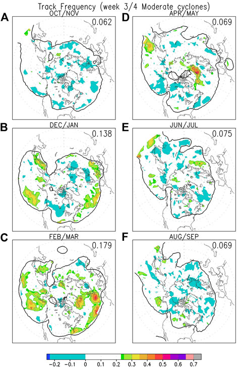
FIGURE 11. Same as Figure 8, but for weeks 3-4 hindcasts of cyclone track frequency of moderate cyclones.
The results for track amplitude for moderate cyclones for winter are shown in Figures 12A,B. Statistically significant ACC scores are only found near Iceland. The ACC scores for model predictions of all cyclones are shown in the remaining panels of Figure 12. Similar to the results for week 2, the ACC scores for predicting the track frequency for all cyclones (Figures 12C,D) are generally lower than those for the track frequency of moderate cyclones (Figures 11B,C), while those for predicting the track amplitude of all cyclones (Figures 12E,F) are higher than those for the track amplitude of moderate cyclones (Figures 12A,B).
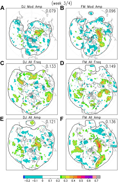
FIGURE 12. (A) ACC scores for weeks 3-4 hindcasts of cyclone amplitude of moderate cyclones for early winter (December/January); (B) Same as (A) but for late winter (February/March); (C,D): Same as (A, B) but for weeks 3-4 hindcasts of cyclone track frequency of al cyclones; (E,F): Same as (A,B) but for weeks 3-4 hindcasts of cyclone amplitude of all cyclones.
How about deep cyclones (those with central pressure below 970 hPa)? Results for the track density of deep cyclones are shown in Figures 10D–F. Out in the subseasonal timescale, models show some ability to predict the frequency of deep cyclones near Iceland during late winter (Figure 10F), likely leveraging model ability to predict both the frequency and amplitude of cyclones over that region (Figures 11C, 12B,F).
Overall, models show little ability to predict cyclone track statistics for weeks 3-4, and the ACC scores for track statistics are much lower than those for variance statistics shown in Figure 5.
As discussed in CORMAX Between Storm Track Metrics and Weather Section, CORMAX (Figure 2) between a weather element (e.g. precipitation) and a storminess metric (e.g. ECApp) quantifies how strongly the variations in that weather element at that grid point correlate with the storminess metric in the vicinity of that grid point. CORMAX between precipitation and ECApp is shown in Figure 2A. The correlation between precipitation and ECApp is high over the western part of the U.S. extending into the eastern Pacific. It is also high over much of western Europe extending into eastern Atlantic, as well as parts of Siberia and the coastal regions of northeastern Asia. Over these regions, the correlation generally exceeds 0.6, and exceeds 0.7 over parts of the region. Correlation between GPCP precipitation and ECApp is generally low over the western parts of the ocean basins. We have also computed CORMAX using ERA5 monthly precipitation (see Supplementary Figure S29A). The pattern is quite similar, except that the correlation between ERA5 precipitation and ECApp is generally higher, especially over the oceans.
CORMAX between the high wind index (the 95th-percentile wind in each month; see Reanalysis and Observational Data Section) and ECApp is shown in Figure 2B. The correlation between this high wind index and ECApp is generally high over much of the main storm track regions. We have also examined CORMAX based on the monthly frequency of occurrence of gale force wind (wind speed >17.2 m/s), and the correlation between this high wind index and ECApp is also generally high over the main oceanic storm track (see Supplementary Figure S29B). Note that the 95th percentile high wind index is relevant over both land and ocean, while over land, 10-m wind speed rarely exceeds gale force and hence the gale force wind index is only relevant over oceanic regions.
Previous studies (e.g. Osburn et al., 2018; Yau and Chang 2020) have shown that cyclone track statistics are also well correlated with precipitation and high wind. The one-point correlation between the GPCP precipitation at the California reference point and cyclone track frequency for moderate cyclones (minimum SLP <1000 hPa) is shown in Figure 1C. It can be seen that precipitation over California is moderately correlated with cyclone track frequency just offshore of the U.S. west coast. The correlation is lower than that between precipitation and ECApp (Figure 1A), consistent with the results of Yau and Chang (2020). Yau and Chang (2020) also showed that the correlation between precipitation and track frequency is higher if cyclones are defined by 850 hPa vorticity anomalies instead of by SLP, likely reflecting the dynamic impact of differential vorticity advection in forcing rising motion.
CORMAX for all grid boxes relating precipitation at that grid box to cyclone track frequency is shown in Figure 2C. Compared to that between precipitation and ECApp (Figure 2A), the pattern is similar, but the overall correlation is lower. Again, moderate correlations can be found near the U.S. west coast, the western and northern parts of Europe, central Siberia, and the northeastern part of Asia.
CORMAX relating the high wind index at all grid boxes to cyclone track frequency is shown in Figure 2D, showing generally lower correlations between high winds and track frequency than those between high winds and ECApp (Figure 2B). This is also the case if the frequency of gale force wind is used as the high wind index (Supplementary Figure S29). This is not surprising, since the occurrence of high winds not only depends on the proximity of a cyclone center, but is also related to cyclone intensity. Cyclone track frequency does not take into account cyclone intensity, but ECApp is an integrated measure of storminess that contains the information of both cyclone frequency and amplitude, hence it is not surprising that ECApp is better correlated to weather elements such as precipitation and high wind compared to cyclone frequency. We will discuss this further in Combining Cyclone Frequency and Intensity Information Section.
One important parameter for accumulating cyclone track statistics is the radius used to accumulate cyclone statistics around the center of each grid box. Extratropical cyclones generally cover a broad region, and previous studies found that the maximum wind and heavy precipitation generally extends out to about 500 km or more away from the cyclone center (e.g. Chang and Song 2006; Field and Wood 2007; Bengtsson et al., 2009). Thus, it is not surprising that many previous studies used 500 km radius or 5-degree polar cap (∼555 km radius) to accumulate cyclone statistics (e.g. Sinclair, 1997; Grise et al., 2013; Guo et al., 2017; Yau and Chang, 2020). Nevertheless, some studies used a larger radius–for example, Pinto et al. (2005) used a radius of 7.5° (∼832 km). There are also some studies that used a smaller area–for example, Serreze and Barrett (2008) used 250 km grid boxes, although the statistics are smoothed with adjacent grid boxes, thus effectively using larger grid boxes.
We tested the sensitivity of our results to accumulating statistics using a radius of 500 km versus a radius of 250 km. We examined how well models can predict the track statistics, as well as how well correlated the track statistics are with precipitation and high winds. The results are summarized in Table 1, which shows ACC and CORMAX values averaged over the region 180–0 °W, 25–70 °N. Comparing the second and third rows, we can see that cyclone track frequency accumulated using a radius of 500 km is better predicted than that accumulated using a radius of 250 km, which is likely because statistics accumulated using a radius of 250 km is much noisier. The correlation between weather and track statistics is also slightly better for track statistics accumulated using a radius of 500 km, which is not surprising given that weather associated with cyclones usually extends out to 500 km away from the cyclone center. Given these results, we have decided to use a radius of 500 km to accumulate cyclone statistics. Note that, as discussed in the Supplementary Text S2.1, while many of the average ACC values for weeks 3-4 listed in column 3 of Table 1 are less than the significant ACC value for individual grid points (0.23), because these values are averages of ACC values over a large number of grid points, all these values are statistically significant at the 95% level based on a Monte Carlo field significance test.
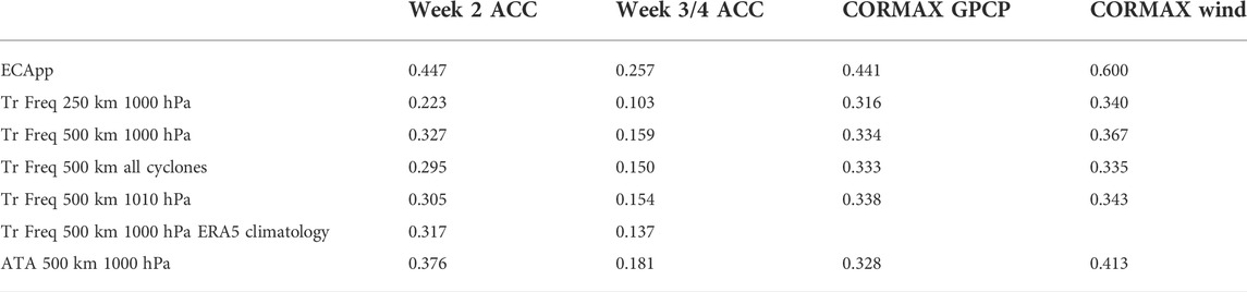
TABLE 1. Summary statistics for different storminess indices averaged over 180–0 °W, 25–70 °N for DJFM.
In Results Section, we showed that the models predict cyclone track frequency better for moderate cyclones than for all cyclones. This is confirmed by the statistics shown in Table 1 (compare rows 3 and 4). The average CORMAX values for GPCP precipitation for both types of track statistics are similar, but The CORMAX for high wind events is slightly higher for the frequency of moderate cyclones than for all cyclones, which is not surprising since the highest winds experienced at each grid box are likely related to the stronger cyclones rather than weak cyclones. We have also computed the statistics for keeping cyclones with SLP <1010 hPa instead of 1000 hPa. The summary statistics are shown in row 5 of Table 1. Compared to row 3, the results are rather similar, but the statistics for keeping cyclones with SLP <1000 hPa are slightly better. After consultation with forecasters, we decided to generate cyclone statistics for moderate cyclones (SLP <1000 hPa) for our outlook tool.
When we computed the ACC scores between predicted and reanalysis storminess metrics, bias correction was applied by computing model predicted anomalies using the models’ own climatologies. The biases in model climatologies are shown in Supplemental Figures S3–S10, S13–S20, S22–S23, S25–28.
We have tested how much improvement this simple bias correction provides, by computing model anomalies not by subtracting off the model’s own climatology, but by subtracting off ERA5 climatology–i.e. no bias correction is performed. The results are shown in row 6 of Table 1. We can see that as expected, the ACC scores are lower compared to those shown in row 3 when bias correction is made, but only slightly lower. This demonstrates that while bias correction does improve the quality of the model forecasts, it is not essential for the model to show positive skill.
In Results Section, we saw that the ACC scores for ECApp (SLP variance statistics) are much higher than those for track frequency or amplitude/intensity. We hypothesize that one contributing factor might be related to the fact that ECApp combines information from cyclone frequency and amplitude, and since models show some ability to predict both frequency and amplitude, the combination of the two might be more predictable.
One way of combining cyclone frequency and amplitude is the Accumulated Track Activity (ATA) introduced by Yau and Chang (2020). In short, ATA at any grid box is computed by summing the maximum amplitude reached by all cyclones within 500 km of the center of the grid box over the time period, with each cyclone only counted once at its peak amplitude within the 500 km radius. Following Hoskins and Hodges (2002), in Yau and Chang (2020), cyclones are defined by removing the large-scale background, using spherical spectral decomposition of either SLP or 850 hPa relative vorticity and retaining only the spectral components ≥ T5 (triangular truncation retaining total wavenumber 5 or above). Given this definition, cyclone amplitude is easy to define as the minimum SLP or maximum relative vorticity of the retained anomaly field.
In this work, we use a more traditional way of defining cyclones, by tracking the minima in the total SLP field. Thus it is not entirely clear how to define an amplitude to be accumulated for ATA. Since we are removing the portion of all cyclone tracks with SLP >1000 hPa, one way to define the cyclone amplitude is 1000-SLPmin, where SLPmin is the minimum SLP (in hPa) found at the center of the cyclone. Using this definition, ATA can be readily computed.
The statistics for this metric are summarized by row 7 of Table 1. Compared to the statistics for track frequency (row 3), models predict ATA with higher ACC for both week 2 and weeks 3-4, but the ACC scores are still lower than those for ECApp (row 1). Average CORMAX between GPCP precipitation and ATA is similar to that between GPCP precipitation and track frequency, but the CORMAX between the high wind index and ATA is higher than that between the high wind index and track frequency. This is not surprising since ATA contains information of cyclone intensity which should make it better correlated with high winds than track frequency alone. Nevertheless, the average CORMAX scores for ATA are still substantially lower than those for ECApp (row 1). This is likely in part due to the suboptimal definition of cyclone amplitude, since with this definition, a cyclone with SLPmin equals to 1000 hPa does not contribute to ATA.
Here we have demonstrated that combining cyclone track frequency and amplitude information can result in improved forecasts as well as higher correlations with weather, especially high winds. However, one of the main advantages of considering cyclone track statistics over variance statistics is the additional information provided by these statistics by separating out the information on cyclone frequency and intensity, and combining the information together to form ATA removes these additional information. Hence we have not attempted to fine tune the definition of ATA, and instead encourage users to consider the variance statistics ECApp instead of ATA if only information on the total cyclone activity is needed.
GEFSv12 is an updated version of its predecessor GEFSv11, hence it is of interest to compare their performance in predicting storminess. GEFSv11 data are retrieved from the SubX database, which only provides daily mean data. Since cyclone tracking requires 6-hrly data, we can only compute variance statistics using GEFSv11 data. To directly compare GEFSv12 predictions with those of GEFSv11, the 6-hrly GEFSv12 data are averaged into daily mean data, before ECApp is computed based on Eq. 1.
Since we have shown above that models predict ECApp best in winter, here we compare GEFSv11 and GEFSv12 hindcasts for December to March for weeks 3–4. The ACC values for GEFSv12 hindcasts are shown in Figure 13A, while those for GEFSv11 are shown in Figure 13B. Moderate ACC scores are found in the same regions as those discussed above (Figures 5B,C), and overall GEFSv12 exhibits slightly higher skill than GEFSv11.
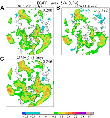
FIGURE 13. (A) ACC scores for weeks 3-4 hindcasts of winter (December-March) SLP variance (ECApp) by GEFSv12 ensemble using daily mean data; (B) Same as (A) but for GEFSv11 ensemble; (C) Same as (A) but for GEFSv12 ensemble using 6-hrly data.
It is also of interest to compare the sensitivity of the model skill to the data frequency, i.e., whether daily mean or 6-hrly data are used to compute ECApp. The ACC for using 6-hrly data for GEFSv12 is shown in Figure 13C. It is clear that the model can predict ECApp computed using 6-hrly data (Figure 13C) better than that computed based on daily mean data (Figure 13A), likely because ECApp is more noisy when computed using daily mean data because of averaging over much fewer time steps.
The week-2 and weeks 3-4 storminess outlook products and CFSR verification are available at the real-time forecast website (https://ftp.cpc.ncep.noaa.gov/hwang/YP/week2/), with a daily update.
The outlook products include the following variables: 1) Storm tracks and track density, storm intensity and duration, 2) Total precipitation, mean SLP, 10-m wind and wind speed, and 3) Day-to-day SLP variance. The website provides GEFSv12, CFSv2, and GEFSv12+CFSv2 combined storminess outlooks. The website also includes regional maps over Alaska/Arctic, North Pacific, North America and North Atlantic.
The outlooks consist of both deterministic forecast (ensemble mean forecast) and probabilistic forecast. The latter is based on the distribution of individual member forecasts. Both the week-2 and weeks 3-4 probabilistic forecasts for precipitation and 10-m wind speed exceeding 75th and 90th percentiles, and storm intensity lower than 990, 980, 970, and 960 hPa are provided.
Verification of the real-time forecasts against the CFSR is provided when the CFSR data are available for the forecast target weeks. Therefore, there is a 16-day delay for the real-time week-2 forecast and 29-day delay for the real-time weeks 3-4 forecast.
In this study, we have evaluated the ability of GEFSv12 and CFSv2 in predicting Northern Hemisphere extratropical storminess for week 2 and weeks 3-4 using 18 years of hindcast data. Both Lagrangian cyclone track statistics, as well as Eulerian SLP variance statistics, have been examined. Our results showed that GEFSv12 generally performs better than CFSv2—one contributing factor is that CFSv2 is a lagged ensemble, including members that are nearly 3 days old, while all GEFSv12 members are initialized at day 0. Overall, we found that the combined GEFSv12/CFSv2 multi-model ensemble consistently outperforms either individual ensemble, thus we focused on evaluating the performance of the combined ensemble.
For week 2, as indicated by the ACC scores, SLP variance is quite well predicted in winter (December to March) over much of the Pacific, parts of North America, much of the Atlantic extending towards Europe, and parts of East Asia. Model predictions are slightly less skillful for spring and fall, and the ACC scores are lowest for summer. For weeks 3-4, the ACC scores are much lower, and rarely exceed 0.5. For winter, moderate scores are found over the areas mentioned above. For spring and fall, models show some ability to predict SLP variance over parts of the central Pacific and parts of eastern North America extending into western Atlantic. Model prediction skill for SLP variance is generally low in summer for weeks 3–4. Our results also show that GEFSv12 exhibits higher skill than its predecessor GEFSv11. To put these results into perspective, the average model ACC scores for predicting SLP variance in weeks 3-4 in winter are slightly lower than those for predicting 2 m temperature over land (∼0.3), and higher than those for predicting precipitation (∼0.1; e.g., Richter et al., 2022). Zheng et al. (2019, 2021) showed that model skill in predicting storminess is mainly associated with the modulations of storminess by ENSO and polar vortex variations. Since both ENSO teleconnections and polar vortex variability are strongest in winter, it is not surprising that models predict storminess best in winter. While this result is not unexpected, our analyses explicitly quantified how much better model predictions are in winter compared to the other seasons.
For track statistics, models show the ability to predict both track frequency and intensity with moderate ACC scores over much of the main storm track regions in week 2. Again, the ACC scores are highest for winter, and lowest for summer. Models predict the frequency of moderate cyclones (those with minimum SLP <1000 hPa) better than the frequency of all cyclones, and show some ability to predict the frequency of deep cyclones (near the Aleutian and Icelandic lows) during fall and winter. For weeks 3-4, models only have some ability to predict the frequency of moderate cyclones over parts of the Pacific and the Atlantic in winter, and some ability to predict deep cyclones near Iceland in late winter, and little ability to predict track statistics for the other seasons. Overall, models predict SLP variance much better than Lagrangian track statistics both for week 2 and weeks 3-4.
In this study, we have assessed model performance based on the ACC score. Some previous studies have assessed model performance based on the RMSE (e.g., Lukens and Berbery, 2019). We have also conducted some assessments based on the MSE. Our results indicate that the 23-member ensemble considered in this study exhibits skill (relative to the no-skill climatological forecasts) based on both the ACC and MSE scores. However, a 1-member CFSv2 hindcast, similar to that analyzed by Lukens and Berbery (2019), exhibits some skill according to the ACC score, but no skill according to the MSE score, consistent with the results of Lukens and Berbery (2019). These results highlight that the ensemble mean forecast performs much better than the forecast by a single member regardless of the assessment metric. These results are discussed in the Supplementary Material (Supplementary Text S2.2).
Our interest in predicting storminess is due to the link between storminess and weather, including precipitation and high winds, especially during the cool season. We have examined the correlation between the storminess metrics and weather indicators in winter. The weather indicators include GPCP precipitation and a high-wind index derived from reanalysis data. Our results indicate that SLP variance is highly correlated with precipitation over the eastern Pacific extending into western North America, eastern Atlantic extending towards western Europe, and the coastal regions of northeastern Asia. SLP variance is also highly correlated with the high wind index over much of the main storm track regions. Correlations of cyclone track frequency and precipitation with the high wind index are also highest over those regions, but are much lower than those for SLP variance.
Generation of cyclone track statistics requires some subjective choices, including the radius for accumulation of cyclone track statistics, and whether to include all cyclones or only include cyclones that are deeper than a certain cutoff limit. Our results indicate that cyclone statistics that are accumulated with a radius of 500 km are better predicted and correlate better with weather indices than those accumulated with a radius of 250 km. We also found that cyclone track frequency for moderate cyclones (those with SLP <1000 hPa) is slightly better predicted and also correlates slightly better with weather indices than cyclone track frequency for all cyclones. Thus, for our outlook tool, we use 500 km to accumulate cyclone statistics, and focus on the statistics of moderate cyclones. The real time outlook webpage is described in Real Time Outlook Tool Web Page Section, and includes forecast information for both SLP variance and track statistics. Given that the operational ensembles have many more members than those used for the hindcast evaluations, we expect that we may find higher skills in operational forecasts. We will monitor the products and update the evaluations using the larger operational ensembles after we have accumulated several seasons of forecast data.
Apart from the ACC scores, we have also generated the seasonal climatology for both SLP variance and cyclone track statistics, and computed the systematic model biases for GEFSv12 and CFSv2 in predicting these storminess metrics. The results, based on ERA5 reanalysis data, are displayed in the Supplementary Material. Results based on CFSR reanalysis data will be posted on the outlook webpage.
Our results show that SLP variance statistics are generally better predicted than cyclone track statistics, and also correlate better with precipitation and high winds. This is probably partly due to the fact that SLP variance combines information from both cyclone track frequency and intensity into one metric. We tested a metric, the Accumulated Track Activity (ATA), that attempts to combine information from both cyclone track frequency and intensity into a single metric, and found that indeed models predict this metric better, and this metric also correlates better with weather (especially high winds) than cyclone track frequency. Nevertheless, the ACC scores as well as the correlation with weather for ATA are still much lower than those for the SLP variance. Given these results, we encourage forecasters and users of our outlook tool to consider the use of SLP variance as an indicator of storminess activity in the subseasonal time scale, unless the application requires specific knowledge about cyclone frequency and/or intensity, which cannot be separately provided by SLP variance statistics.
In this study, we have focused on storminess metrics derived from SLP data, largely because users, including forecasters, are more familiar with cyclones defined by minima in SLP (see, e.g., the surface analysis generated by the Weather Prediction Center). Yau and Chang (2020) examined the correlation between multiple storminess metrics with precipitation and high winds, and found that among Eulerian variance metrics, eddy kinetic energy (EKE) at 850 hPa level correlates slightly better with precipitation than SLP variance, and that cyclone track statistics derived from tracking 850 hPa relative vorticity maxima also correlate better with weather than those derived from SLP data. Results presented in Stan et al. (2022) showed that current S2S models have some ability to predict the MJO modulation of 850 hPa EKE over the Pacific and the Atlantic. Currently we are investigating how well cyclone statistics derived from tracking 850 hPa relative vorticity maxima are predicted by models, as well as whether 850 hPa EKE can serve as a proxy for predicting severe weather such as heavy precipitation and high winds over the subseasonal timescale. Finally, Zheng et al. (2019) showed that for SLP variance, in the subseasonal timescale, the prediction skill is mainly due to models’ ability to predict the storm track response to the modulations of ENSO and polar vortex variability. It would be of interest to see whether this is also the case for the other storminess metrics.
The original contributions presented in the study are included in the article/Supplementary Material, further inquiries can be directed to the corresponding author.
EC and WW conceived the ideas and led the project. EC, YP, and CZ conducted the analyses. EC and YP drafted the paper. All authors provided comments and edits to the final manuscript.
This study is supported by NOAA grant NA20OAR4590315.
The authors would like to thank Di Chen for assisting with the analyses of the variance statistics, and Rui Zhang for helping to access and process ERA5 data. The authors would also like to thank the reviewers for providing comments and suggestions.
YP was employed by the company Earth Resources Technology (ERT), Inc.
The remaining authors declare that the research was conducted in the absence of any commercial or financial relationships that could be construed as a potential conflict of interest.
All claims expressed in this article are solely those of the authors and do not necessarily represent those of their affiliated organizations, or those of the publisher, the editors and the reviewers. Any product that may be evaluated in this article, or claim that may be made by its manufacturer, is not guaranteed or endorsed by the publisher.
The Supplementary Material for this article can be found online at: https://www.frontiersin.org/articles/10.3389/feart.2022.963779/full#supplementary-material
Adler, R. R., Sapiano, M., Huffman, G., Wang, J. J., Gu, G., Bolvin, D., et al. (2018). The global precipitation climatology project (GPCP) monthly analysis (new version 2.3) and a review of 2017 global precipitation. Atmosphere 9, 138. doi:10.3390/atmos9040138
Alexander, L. V., Tett, S. F. B., and Jonsson, T. (2005). Recent observed changes in severe storms over the United Kingdom and Iceland. Geophys. Res. Lett. 32, L13704. doi:10.1029/2005gl022371
Ashley, W. S., and Black, A. W. (2008). Fatalities associated with nonconvective high wind events in the United States. J. Appl. Meteorol. Climatol. 47, 717–725. doi:10.1175/2007jamc1689.1
Atger, F. (1999). The skill of ensemble prediction systems. Mon. Wea. Rev. 127, 1941–1953. doi:10.1175/1520-0493(1999)127<1941:tsoeps>2.0.co;2
Baldwin, M. P., and Dunkerton, T. J. (2001). Stratospheric harbingers of anomalous weather regimes. Science 294, 581–584. doi:10.1126/science.1063315
Bengtsson, L., Hodges, K. I., and Keenlyside, N. (2009). Will extratropical storms intensify in a warmer climate? J. Clim. 22, 2276–2301. doi:10.1175/2008jcli2678.1
Berko, J., Ingram, D. D., Saha, S., and Parker, J. D. (2014). Deaths attributed to heat, cold, and other weather events in the United States, 2006-2010. National health statistics reports No. 76. Hyattsville, MD: National Center for Health Statistics.
Chang, E. K. M. (2013). CMIP5 projection of significant reduction in extratropical cyclone activity over North America. J. Clim. 26, 9903–9922. doi:10.1175/jcli-d-13-00209.1
Chang, E. K. M., and Song, S. (2006). The seasonal cycles in the distribution of precipitation around cyclones in the Western North Pacific and Atlantic. J. Atmos. Sci. 63, 815–839. doi:10.1175/jas3661.1
Chang, E. K. M., Zheng, C., Lanigan, P., Yau, A. M. W., and Neelin, J. D. (2015). Significant modulation of variability and projected change in California winter precipitation by extratropical cyclone activity. Geophys. Res. Lett. 42, 5983–5991. doi:10.1002/2015gl064424
Chang, E. K. M., Ma, C.-G., Zheng, C., and Yau, A. M. W. (2016). Observed and projected decrease in Northern Hemisphere extratropical cyclone activity in summer and its impacts on maximum temperature. Geophys. Res. Lett. 43, 2200–2208. doi:10.1002/2016gl068172
Charles, M. E., and Colle, B. A. (2009). Verification of extratropical cyclones within the NCEP operational models. Part I: Analysis errors and short-term NAM and GFS forecasts. Weather Forecast. 24, 1173–1190. doi:10.1175/2009waf2222169.1
Colle, B. A., Buonaiuto, F., Bowman, M. J., Wilson, R. E., Flood, R., Hunter, R., et al. (2008). New York City’s vulnerability to coastal flooding. Bull. Amer. Meteor. Soc. 89, 829–842. doi:10.1175/2007bams2401.1
Deng, Y., and Jiang, T. (2011). Intraseasonal modulation of the North Pacific storm track by tropical convection in boreal winter. J. Clim. 24, 1122–1137. doi:10.1175/2010jcli3676.1
Eichler, T., and Higgins, W. (2006). Climatology and ENSO-related variability of north American extratropical cyclone activity. J. Clim. 19, 2076–2093. doi:10.1175/jcli3725.1
Feser, F., Barcikowska, M., Krueger, O., Schenk, F., Weisse, R., and Xia, L. (2015). Storminess over the north atlantic and North-Western Europe – a review. Q. J. R. Meteorol. Soc. 141, 350–382. doi:10.1002/qj.2364
Field, P. R., and Wood, R. (2007). Precipitation and cloud structure in midlatitude cyclones. J. Clim. 20, 233–254. doi:10.1175/jcli3998.1
Froude, L. S., Bengtsson, L., and Hodges, K. I. (2007). The prediction of extratropical storm tracks by the ECMWF and NCEP ensemble prediction systems. Mon. Weather Rev. 135, 2545–2567. doi:10.1175/mwr3422.1
Froude, L. S. (2010). Tigge: Comparison of the prediction of northern hemisphere extratropical cyclones by different ensemble prediction systems. Weather Forecast. 25, 819–836. doi:10.1175/2010waf2222326.1
Grise, K. M., Son, S., and Gyakum, J. R. (2013). Intraseasonal and interannual variability in North American storm tracks and its relationship to equatorial Pacific variability. Mon. Weather Rev. 141, 3610–3625. doi:10.1175/mwr-d-12-00322.1
Guan, H., Zhu, Y., Sinsky, E., Fu, B., Li, W., Zhou, X., et al. (2022). GEFSv12 reforecast dataset for supporting subseasonal and hydrometeorological applications. Mon. Weather Rev. 150, 647–665. doi:10.1175/mwr-d-21-0245.1
Guo, Y., Shinoda, T., Lin, J., and Chang, E. K. M. (2017). Variations of Northern Hemisphere storm track and extratropical cyclone activity associated with the Madden-Julian Oscillation. J. Clim. 30, 4799–4818. doi:10.1175/jcli-d-16-0513.1
Hersbach, H., Bell, B., Berrisford, P., Hirahara, S., Nicolas, J., Peubey, C., et al. (2020). The ERA5 global reanalysis. Quart. J. R. Meteoro. Soc. 146, 1999–2049. doi:10.1002/qj.3803
Hodges, K. I. (1994). A general method for tracking analysis and its application to meteorological data. Mon. Wea. Rev. 122, 2573–2586. doi:10.1175/1520-0493(1994)122<2573:agmfta>2.0.co;2
Hodges, K. I., Lee, R. W., and Bengtsson, L. (2011). A comparison of extratropical cyclones in recent reanalyses ERA-interim, NASA MERRA, NCEP CFSR, and JRA-25. J. Clim. 24, 4888–4906. doi:10.1175/2011jcli4097.1
Hoskins, B. J., and Hodges, K. I. (2002). New perspectives on the Northern Hemisphere winter storm tracks. J. Atmos. Sci. 59, 1041–1061. doi:10.1175/1520-0469(2002)059<1041:npotnh>2.0.co;2
Kocin, P. J., Weiss, A. D., and Wagner, J. J. (1988). The great Arctic outbreak and East Coast blizzard of February 1899. Weather Forecast. 3, 305–318. doi:10.1175/1520-0434(1988)003<0305:tgaoae>2.0.co;2
Kunkel, K. E., Easterling, D. R., Kristovich, D. A. R., Gleason, B., Stoecker, L., and Smith, R. (2012). Meteorological causes of the secular variations in observed extreme precipitation events for the conterminous United States. J. Hydrometeorol. 13, 1131–1141. doi:10.1175/jhm-d-11-0108.1
Lackmann, G. (2011). Midlatitude synoptic meteorology: Dynamics, analysis, and forecasting. American Meteorological Society, 345.
Livezey, R. E., and Chen, W. Y. (1983). Statistical field significance and its determination by Monte Carlo techniques. Mon. Weather Rev. 111, 46–59. doi:10.1175/1520-0493(1983)111<0046:sfsaid>2.0.co;2
Lukens, K. E., and Berbery, E. H. (2019). Winter storm tracks and related weather in the NCEP Climate Forecast System weeks 3-4 reforecasts for North America. Weather Forecast. 34, 751–772. doi:10.1175/waf-d-18-0113.1
Ma, C.-G., and Chang, E. K. M. (2017). Impacts of storm-track variations on wintertime extreme weather events over the continental United States. J. Clim. 30, 4601–4624. doi:10.1175/jcli-d-16-0560.1
Neu, U., Akperov, M. G., Bellenbaum, N., Benestad, R., Blender, R., Caballero, R., et al. (2013). Imilast: A community effort to intercompare extratropical cyclone detection and tracking algorithms. Bull. Am. Meteorol. Soc. 94, 529–547. doi:10.1175/bams-d-11-00154.1
Osburn, L., Keay, K., and Catto, J. L. (2018). Projected change in wintertime precipitation in California using projected changes in extratropical cyclone activity. J. Clim. 31, 3451–3466. doi:10.1175/jcli-d-17-0556.1
Paciorek, C. J., Risbey, J. S., Ventura, V., and Rosen, R. D. (2002). Multiple indices of Northern Hemisphere cyclone activity, winters 1949–99. J. Clim. 15, 1573–1590. doi:10.1175/1520-0442(2002)015<1573:mionhc>2.0.co;2
Pegion, K., Kirtman, B. P., Becker, E., Collins, D. C., LaJoie, E., Burgman, R., et al. (2019). The subseasonal experiment (SubX): A multi-model subseasonal prediction experiment. Bull. Am. Meteorol. Soc. 100, 2043–2060. doi:10.1175/bams-d-18-0270.1
Pfahl, S., and Wernli, H. (2012). Quantifying the relevance of cyclones for precipitation extremes. J. Clim. 25, 6770–6780. doi:10.1175/jcli-d-11-00705.1
Pinto, J. G., Spangehl, T., Ulbrich, U., and Speth, P. (2005). Sensitivities of a cyclone detection and tracking algorithm: Individual tracks and climatology. Meteorol. Z. 14, 823–838. doi:10.1127/0941-2948/2005/0068
Richter, J. H., Glanville, A. A., Edwards, J., Kauffman, B., Davis, N. A., Jaye, A., et al. (2022). Subseasonal Earth system prediction with CESM2. Weather Forecast. 37, 797–815. doi:10.1175/waf-d-21-0163.1
Saha, S., Moorthi, S., Pan, H. L., Wu, X., Wang, J., Nadiga, S., et al. (2010). The NCEP climate forecast system reanalysis. Bull. Amer. Meteor. Soc. 91, 1015–1058. doi:10.1175/2010BAMS3001.1
Saha, S., Moorthi, S., Wu, X., Wang, J., Nadiga, S., Tripp, P., et al. (2014). The NCEP climate forecast system version 2. J. Clim. 27, 2185–2208. doi:10.1175/JCLI-D-12-00823.1
Salmun, H., Molod, A., Wisniewska, K., and Buonaiuto, F. S. (2011). Statistical prediction of the storm surge associated with cool-weather storms at the battery, New York. J. Appl. Meteorol. Climatol. 50, 273–282. doi:10.1175/2010jamc2459.1
Serreze, M. C., and Barrett, A. P. (2008). The summer cyclone maximum over the central arctic ocean. J. Clim. 21, 1048–1065. doi:10.1175/2007jcli1810.1
Serreze, M. C. (1995). Climatological aspects of cyclone development and decay in the Arctic. Atmosphere-Ocean 33, 1–23. doi:10.1080/07055900.1995.9649522
Sinclair, M. R. (1997). North Atlantic storm track variability and its association to the North Atlantic Oscillation and climate variability of northern Europe. J. Clim. 10, 1635–1647. doi:10.1175/1520-0442(1997)010<1635:nastva>2.0.co;2
Stan, C., Zheng, C., Chang, E. K-M., Domeisen, D. I. V., Garfinkel, C. I., Jenney, A. M., et al. (2022). Advances in the prediction of MJO Teleconnections in the S2S forecast systems. Bull. Amer. Meteoro. Soc. 103, E1426–E1447. doi:10.1175/BAMS-D-21-0130.1
Straus, D. M., and Shukla, J. (1997). Variations of midlatitude transient dynamics associated with ENSO. J. Atmos. Sci. 54, 777–790. doi:10.1175/1520-0469(1997)054<0777:vomtda>2.0.co;2
Vitart, F., Ardilouze, C., Bonet, A., Brookshaw, A., Chen, M., Codorean, C., et al. (2017). The subseasonal to seasonal (S2S) prediction project database. Bull. Am. Meteorol. Soc. 98, 163–173. doi:10.1175/bams-d-16-0017.1
Wallace, J. M., Lim, G.-H., and Blackmon, M. L. (1988). Relationship between cyclone tracks, anticyclone tracks and baroclinic waveguides. J. Atmos. Sci. 45, 439–462. doi:10.1175/1520-0469(1988)045<0439:rbctat>2.0.co;2
Walter, K., and Graf, H.-F. (2005). The North Atlantic variability structure, storm tracks, and precipitation depending on the polar vortex strength. Atmos. Chem. Phys. 5, 239–248. doi:10.5194/acp-5-239-2005
Wang, J., Kim, H.-M., and Chang, E. K. M. (2018). Interannual modulation of Northern Hemisphere winter storm tracks by the QBO. Geophys. Res. Lett. 45, 2786–2794. doi:10.1002/2017gl076929
Yang, X., Vecchi, G. A., Gudgel, R. G., Delworth, T. L., Zhang, S., Rosati, A., et al. (2015). Seasonal predictability of extratropical storm tracks in GFDL’s high-resolution climate prediction model. J. Clim. 28, 3592–3611. doi:10.1175/jcli-d-14-00517.1
Yau, A. M. W., and Chang, E. K. M. (2020). Finding storm track activity metrics that are highly correlated with weather impacts. Part I: Frameworks for evaluation and accumulated track activity. J. Clim. 33, 10169–10186. doi:10.1175/jcli-d-20-0393.1
Zhang, G., Murakami, H., Cooke, W. F., Wang, Z., Jia, L., Lu, F., et al. (2021). Seasonal predictability of baroclinic wave activity. npj Clim. Atmos. Sci. 4, 50. doi:10.1038/s41612-021-00209-3
Zheng, C., Chang, E. K. M., Kim, H.-M., Zhang, M., and Wang, W. (2018). Impacts of the Madden-Julian Oscillation on storm track activity, surface air temperature, and precipitation over North America. J. Clim. 31, 6113–6134. doi:10.1175/jcli-d-17-0534.1
Zheng, C., Chang, E. K. M., Kim, H., Zhang, M., and Wang, W. (2019). Subseasonal to seasonal prediction of wintertime Northern Hemisphere extratropical cyclone activity by S2S and NMME models. J. Geophys. Res. Atmos. 124, 12057–12077. doi:10.1029/2019jd031252
Zheng, C., Chang, E. K. M., Kim, H., Zhang, M., and Wang, W. (2021). Subseasonal prediction of wintertime Northern Hemisphere extratropical cyclone activity by SubX and S2S models. Weather Forecast. 36, 75–89. doi:10.1175/waf-d-20-0157.1
Zhou, X., Zhu, Y., Hou, D., Luo, Y., Peng, J., and Wobus, D. (2017). The NCEP global ensemble forecast system with the EnKF initialization. Wea. Forecast. 32, 1989–2004.
Keywords: extratropical storminess, subseasonal prediction, forecast verification, ensemble prediction, cyclones, storm tracks
Citation: Chang EKM, Pan Y, Wang W and Zheng C (2022) Developing and evaluating week 2 and weeks 3-4 outlook tools for extratropical storminess. Front. Earth Sci. 10:963779. doi: 10.3389/feart.2022.963779
Received: 07 June 2022; Accepted: 03 October 2022;
Published: 17 October 2022.
Edited by:
Zhuo Wang, University of Illinois at Urbana-Champaign, United StatesReviewed by:
Gan Zhang, Citadel LLC, United StatesCopyright © 2022 Chang, Pan, Wang and Zheng. This is an open-access article distributed under the terms of the Creative Commons Attribution License (CC BY). The use, distribution or reproduction in other forums is permitted, provided the original author(s) and the copyright owner(s) are credited and that the original publication in this journal is cited, in accordance with accepted academic practice. No use, distribution or reproduction is permitted which does not comply with these terms.
*Correspondence: Edmund K. M. Chang, a2FyLmNoYW5nQHN0b255YnJvb2suZWR1
Disclaimer: All claims expressed in this article are solely those of the authors and do not necessarily represent those of their affiliated organizations, or those of the publisher, the editors and the reviewers. Any product that may be evaluated in this article or claim that may be made by its manufacturer is not guaranteed or endorsed by the publisher.
Research integrity at Frontiers
Learn more about the work of our research integrity team to safeguard the quality of each article we publish.