A multi-model fitting algorithm for extracting a fracture network from microseismic data

Fractures are increasingly employed in tectonic movement and earthquake risk analyses. Because fracture connectivity influences fluid flow pathways and flow rates, fractures are studied to evaluate sites for CO₂ sequestration, radioactive waste storage and disposal, petroleum production, and geothermal energy applications. Discrete fracture networks are an effective method for imaging fractures in three-dimensional geometric models and for analyzing the fluid behavior that cause movements in fracture zones. Microseismic event monitoring data can be used to analyze the event source mechanisms and the geometry, distribution, and orientation of the fractures generated during the event. This study proposes a method for simultaneously imaging multi-fracture networks using microseismic monitoring data. The random sample consensus and propose, expand, and re-estimate labels algorithms commonly used in multi-model fitting were integrated to produce an upgraded method that accommodates geophysical data for faster and more accurate simultaneous multi-fracture model imaging within a point cloud. The accuracy of the method was improved using circular calculation and density-based spatial clustering of applications with noise, such that the estimated fracture orientations correspond well to those at the actual locations. The proposed algorithm was applied to synthetic data to assess the impact of considering orientation and outlier data on the model results. The errors in the results when considering orientation were 1.32% and 0.83% for the strike and dip angles, respectively, and those without considering were 20.23% and 24.63% respectively. In addition, the errors in the results obtained from data containing many outliers were 1.89% and 1.64% for the strike and dip angles, respectively. Field microseismic data were also used to depict fractures representing the dominant orientation, and the errors of the strike and dip angle estimates were 2.89% and 2.83%, respectively. These results demonstrate the suitability of the algorithm for fast and accurate field data modeling.

1 Introduction

Fractures form when the stress exceeds the rock strength, causing the rock to split into separate pieces. A fracture can be classified as a fault if the relative rock displacement is parallel to the fracture direction or as a joint if there is no relative displacement (Mitcham, 1963; Gudmundsson, 2011). Fault planes represent structurally vulnerable subsurface areas that require earthquake risk analysis and the determination of large-scale structure safety. Joints are useful for tectonic movement analysis because they can be used to estimate changes caused by stress after rock formation. Therefore, fracture analysis studies have been widely conducted in many disciplines to identify subsurface structures.

Understanding subsurface fracture connectivity is vital for analyzing fluid flow pathways. Numerous studies have conducted core analysis and numerical modeling of groundwater flow through natural fractures (Raven and Gale, 1985; Kwicklis and Healy, 1993; Mayer and Sharp, 1998). In the petroleum industry, hydraulic fracturing is used to improve oil and gas recovery and geothermal energy production, as well as to create artificial fractures for improving subsurface connectivity (Valko and Economides, 2001; Montgomery and Smith, 2010; Zhang et al., 2010).

Microseismic events are very weak earthquakes with a negative moment magnitude that occur on very small spatial scales, and are generated by anthropogenic changes to the natural stress-strain state of formations, such as by hydraulic fracturing, or by natural forces, such as tectonic motions. Microseismic events associated with hydraulic fracturing generally occur in three areas: parent hydraulic fracture side-wall because of the leakage of the pressurized fluid, critically stressed natural fracture, and close to the hydraulic fracturing tip (Busetti et al., 2014). Microseismic monitoring is an important tool for identifying, positioning, and characterizing these events, which can provide information on the growth patterns of fractures induced by high-pressure fluid injection and overall dimensions (Economides and Nolte, 2000; Warpinski et al., 2013). Thus, uncertainties can be analyzed for individual events and leakage events that are not associated with major fracture networks by estimating the extent of microseismic event clouds.

Discrete fracture networks (DFNs) are widely used to analyze fracture connectivity. DFNs can be used to image and model individual three-dimensional (3D) fractures to evaluate the changes in their geometry and behaviors of associated fluids (Dershowitz and Fidelibus, 1999; Li and Lee, 2008; Hyman et al., 2015). They can be constructed in many ways, such as by linking fracture imaging to seismic activity based on microseismic monitoring data (Fadakar Alghalandis et al., 2013) or the source mechanism (Yu et al., 2016; Yu et al., 2020). They are useful because they can identify and display fracture locations solely based on microseismic data. However, fracture orientations determined solely from microseismic event locations often exhibit poor accuracy. Therefore, it is necessary to enhance the reliability of fracture orientation data by incorporating the strike and dip angles at the event location. However, no method for extracting multiple fracture network models has been developed so far.

A method for extracting points associated with each fracture is required to image a DFN in a 3D point cloud, such as the location of a microseismic event. Complementary computer vision techniques have been developed for this purpose, including the widely used Random Sample Consensus (RANSAC) (Fischler and Bolles, 1981) and Hough transform (Duda and Hart, 1972) algorithms. Although these techniques are appropriate for locating a point within the cloud that easily meets specific threshold conditions, the input variables, computation time, and sequential model estimation remain problematic. Isack and Boykov developed the Propose, Expand, and Re-estimate Labels (PEARL) energy-based multi-model optimization algorithm to resolve these issues (Isack and Boykov, 2011). This algorithm iteratively estimates inliers and model parameters based on a global regularization function. As PEARL lowers the variable dependency, it effectively reduces the computation time, and allows simultaneous multi-fracture imaging; however, as only the distance energy between feature points in the image is utilized, it is difficult to consider the direction in three dimensions.

This study proposes a method for imaging fractures using microseismic data based on the multi-fitting algorithm, and represents an improvement over the existing PEARL algorithm for geophysical data systems. This approach integrates microseismic event locations and fracture orientations to enhance the reliability and accuracy of fracture imaging. To confirm the effectiveness of proposed method, a synthetic model simulating microseismic event locations was created and the resulting fracture images were compared, taking into account the influence of orientation and outlier data. The applicability of the proposed method was also tested using field data provided by a geothermal data repository (http://gdr.openei.org/submitssi-ons/1091) operated by the Department of Energy (DOE) Geothermal Technology Office (Gritto et al., 2018).

2 Methodology

2.1 RANSAC algorithm

The RANSAC algorithm (Fischler and Bolles, 1981) was developed to detect simple shapes such as lines, circles, and planes within a point cloud through the iterative estimation of model parameters by randomly sampling data points for consensus. A simple RANSAC algorithm for a microseismic event involves the following steps.

1) A plane model is generated by randomly selecting three points from the event location data.

2) The distances between the generated fracture planes and all other points are calculated.

3) Inlier points are selected from among the threshold distance ($t_d$) parameter values.

4) If the number of inlier points is greater than the number of threshold points ($t_p$), or the minimum number of points required extracting the plane model, then only these points are used to refit the generated plane.

5) The objective function is updated,

$O={\displaystyle \sum }_{p=\mathit{1}}^{n_p}\left(distance\right)/n_p(1)$

where $n_p$ is the number of inliers, and the record is the most effective if $O_k<O_{k-\mathit{1}}$, where $k$ is the iteration counter.

6) The process is then restarted from Step 2) until the desired iteration is attained.

The number of iterations ($n_k$) for optimal results in RANSAC must be chosen sufficiently to ensure the probability that at least one of the point datasets contains only inliers, and is generally determined as follows

$n_k=\frac{\log \left(1-a\right)}{\log \left(1-{\left(1-b\right)}^r\right)}(2)$

where, $b$ is the probability of success, $a$ represents the probability that any selected data point is an outlier, and $r$ is the number of points used to generate the model (2 and 3 for a line and plane, respectively).

Although RANSAC has mainly been applied in image processing and computer vision, its capability to extract a model from a point cloud can be exploited to image fractures based on seismic event location data. Thus, RANSAC can robustly estimate the model parameters with good accuracy, even if there are many outliers. However, the algorithm involves a high computational load because it utilizes random models, which can require a large number of iterations, and the values of several input parameters are set by the user, which significantly influences the results. RANSAC selects only one optimal model from the iterative random sampling models in a sequential estimation process. Therefore, the dataset used to estimate a model is disregarded before a new model is obtained in the next iteration. Therefore, simultaneous estimation of multiple models using RANSAC remains challenging.

2.2 PEARL and energy minimization

PEARL (Isack and Boykov, 2011) involves an iterative method similar to RANSAC to extract models from a point cloud. However, unlike the RANSAC model extraction, which of the PEARL algorithm does not rely solely on the threshold distance or number of points within the point cloud. PEARL method aims to minimize the function of energy and is generally possible through fewer iterations. PEARL is suitable for obtaining multiple models without disregarding the previously used data in subsequent iterations.

Geometric multi-model fitting using PEARL can be formalized through an optimal labeling problem, where each data point $p$ belongs to a separate label, $L_p$. The PEARL algorithm was designed for multi-model extraction that minimizes the energy function $E\left(\mathcal{L}\right)$ by labeling $\mathcal{L}$ as $\left\{L_p|p\in P\right\}$, as follows (Isack and Boykov, 2011; Delong et al., 2012).

$E\left(\mathcal{L}\right)={{\displaystyle \sum }}_p\Vert p-L_p\Vert +\lambda \cdot {{\displaystyle \sum }}_{\left(p,q\right)\in \mathcal{N}}{\omega }_{pq}\cdot \delta \left(L_p{\ne L}_q\right)(3)$

The first term on the right side of Eq. 3 represents a geometric measurement of the data, which is calculated using the distance errors between points assigned to the label and the associated model; $p$ is a point belonging to dataset $P$, $L_p$ is the label associated with point $p$, including the model parameter, and $\Vert p-L_p\Vert$ represents the Euclidean distance between a point and its associated label. As this distance decreases, the probability of extracting the model by using $L_p$ to which point $p$is assigned, increases. By contrast, as the distance increases, the probability decreases, and the label associated with point $p$ may also change.

The second term of Eq. 3 is used for smoothing, where $\mathcal{N}$ represents a set of neighboring points, $\left(p,q\right)\in \mathcal{N}$ indicates that points $p$ and $q$are neighboring points, and $L_p$ and $L_q$are the labels associated with $p$ and $q$, respectively. The value of $\delta \left(L_p{\ne L}_q\right)$ is 0 when $L_p$ and $L_q$are assigned to the same label, and 1 when they are assigned to different labels. Thus, a discontinuity penalty is applied when neighboring points are assigned to different labels, and assigning neighboring points to the same label is encouraged.

The weight of the discontinuity penalty, ${\omega }_{pq}$is expressed as follows.

${\omega }_{pq}=\mathit{exp}-\frac{{\Vert p-q\Vert }^2}{{\xi }^2}(4)$

where $\xi$ and $\lambda$ are empirical constants and $\Vert p-q\Vert$represents the Euclidean distance between points $p$ and $q.$

The original PEARL algorithm comprises three steps: propose, expand, and re-estimate. A simplified flowchart of the algorithm is shown in Figure 1. The operations in each step can be summarized as follows.

FIGURE 1

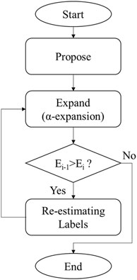
FIGURE 1. Schematic diagram of the original Propose, Expand, and Re-estimate Labels (PEARL) algorithm.

1) In the propose step, the data are randomly sampled as in RANSAC to generate the initial label set ($L_o$) for a predefined number of models.

2) In the expand step, $\alpha$-expansion (Boykov et al., 2001) is performed using an arbitrary label, $\alpha$, assigned to a generated $L_i$ for energy minimization using Eq. 3. In this step, the spatially consistent label containing the largest number of inliers is obtained through expansion between labels.

3) During the operation of the iterative algorithm, if energy minimization is not achieved during the expand step, then the output of the final label is required, followed by the termination of the algorithm.

4) In contrast, if energy minimization is achieved, the points assigned to each label are used for re-estimation. The existing label set and model parameters are then replaced by a new label set that satisfied the following equation.

${\widehat{L}}_i=\underset{l}{\mathrm{a}\mathrm{r}\mathrm{g}\mathrm{m}\mathrm{i}\mathrm{n}}{{\displaystyle \sum }}_{p\in P\left(L_i\right)}\Vert p-l\Vert (5)$

where $P\left(L_i\right)=\left\{p|L\left(p\right)=L_i\right\}$represents the set of points $p$assigned to label $L_i,$followed by a return to the expand step using the re-estimated labels in the next iterative step: $i=\left(i+\mathit{1}\right)$.

Although the conventional PEARL algorithm is suitable for extracting multi-models from a point cloud, extraction in a full 3D domain using image processing has received limited attention to date. Considering that event location data acquired from the surface include complex and sporadically generated point clouds with many outliers, optimal model extraction is challenging, particularly in terms of increased computation time.

2.3 GARNET algorithm

In this study, the efficiency and accuracy of the original PEARL algorithm were improved for fracture imaging using only the seismic event location and fracture orientation data. The developed algorithm is named as geometric model-fitting algorithm for fracture network (GARNET). In contrast to the original PEARL estimation model, which relies solely on the distances between points and labels, the fracture estimation approach is expected to enhance the model accuracy and reduce the computation time by incorporating fracture orientation data, which can be obtained by analyzing the moment tensor of seismic data recorded by a receiver. This tensor is a mathematical expression of the seismic source, where the displacement at an arbitrary point $\mathbf{x}$ at time $t$, $u_j\left(\mathbf{x},t\right)$ is represented as the convolution of the second-order moment tensor $M_{nk}$ and the Green’s function $G_{jn,k}$(Aki and Richards, 2009), which is expressed as follows.

$u_j\left(\mathbf{x},t\right)=M_{nk}{*G}_{jn,k}(6)$

The moment tensor is symmetrical and comprises six elements characteristic of its source. It is a valuable tool for monitoring earthquakes and microseismic activity because the source mechanism and fault orientations (strike, dip, and rake) can be obtained through its inversion.

Fracture models are created using orientation data acquired from the moment tensor as additional input, employing an algorithm capable of processing such data. Therefore, the orientations associated with a microseismic event and those estimated using the fracture model can be compared to evaluate the accuracy and reliability of the orientation data. The use of orientations that are representative of the event associated with the fracture model represents a faster and more reliable method for comparing the orientations estimated using a model and those of a seismic event. Therefore, methods for calculating the statistical parameters (e.g., mean and variance) of the orientations of multiple events are required. However, circular measurements, such as strike and dip, exhibit fundamentally different characteristics from those of linear measurements. The angles of 0° and 360° represent the same strike orientation, although at opposite locations on a linear scale; therefore, circular measurements require specific analytical methods. In this study, statistical methods (Fisher, 2005; Mardia and Jupp, 2009) were applied to calculate orientations using the following equations.

$C={\displaystyle \sum }_{p=1}^m\cos {\theta }_p,S={\displaystyle \sum }_{p=1}^m\sin {\theta }_p,R^2=C^2+S^2\left(R\ge \mathit{0}\right)(7)$

where $m$ is the number of orientations in a group and $\theta$ is the strike/dip angle associated with the event. The mean orientation $\overline{\theta }$ is the average of all orientations, and is calculated as follows.

$\cos \overline{\theta }=\frac{C}{R},\sin \overline{\theta }=\frac{S}{R}(8)$

$\overline{\theta }=\{\begin{array}{c}{\tan }^{-1}\left(\frac{S}{C}\right)S>0,C>0\\ {\tan }^{-1}\left(\frac{S}{C}\right)+\pi C>0\\ {\tan }^{-1}\left(\frac{S}{C}\right)+\mathit{2}\pi S<0,C<0\end{array}(9)$

The quantity $R$ is the length of the resultant vector, and the mean resultant length associated with the mean direction is expressed as follows.

$\overline{R}=\frac{R}{m}(10)$

These equations can be used to compare the strike/dip angles of multiple events with the estimated fracture orientations.

2.3.1 Initial model and label

In RANSAC, a model satisfying the given constraints is ultimately selected from among randomly extracted models, whereas in GARNET, all randomly generated fracture models are utilized as initial model and associated points are assigned as initial labels. Generally, a higher number of initial random models produce better results. However, rather than increasing the number of models infinitely, predetermining which models involve similar fracture orientations can enhance the accuracy of the results and reduce computation time. Accordingly, the initial label sets were randomly generated within the point cloud by applying a loose distance threshold to the original RANSAC method. The angular difference between the normal vector of the generated plane and mean angle of the events belonging to the plane is calculated as follows.

${\theta }_t={\cos }^{-1}\left(\frac{{\mathbf{v}}_m\cdot {\mathbf{v}}_f}{\Vert {\mathbf{v}}_m\Vert \Vert {\mathbf{v}}_f\Vert }\right)(11)$

where ${\mathbf{v}}_f$ is the normal vector of the plane, ${\mathbf{v}}_m$ is the normal vector of the points in the plane, and ${\theta }_t$ is the angle between the normal vectors.

The minimum angle between the normal vectors was calculated as follows.

${\theta }_m=\min \left\{{\theta }_t,\pi -{\theta }_t\right\}(12)$

Planes exceeding the threshold were eliminated before reconstructing an initial label set with enhanced reliability to determine fracture orientations.

2.3.2 Moment tensor clustering and model elimination

Using the original PEARL algorithm, the energy calculated using Eq. 3 following $\alpha$-expansion was based on the distance between each label and the microseismic event locations assigned to each label; thus, the fracture orientations at event locations were neglected. Many event points were associated with a label based on distance, but exhibited significantly different strike or dip angles relative to the other points. To resolve this issue, a clustering method is applied to the point orientations assigned to each label.

Clustering is a widely used unsupervised learning method that produces data clusters by considering the characteristics of the data, yielding specific points or variables that are representative of the data. Thus, a cluster contains data with similar characteristics, whereas data with different characteristics are classified as different clusters or noise. In this study, the density-based spatial clustering of applications with noise (DBSCAN) method (Ester et al., 1996) was applied to orientation clustering. Unlike other clustering methods that rely on the K-means or similar distance algorithms, DBSCAN is advantageous because it does not require the user to designate the number of clusters. Because of these advantages, it is a clustering algorithm used in various fields such as radar data (Guo et al., 2020), fault diagnosis (Liu et al., 2020), and visual analysis (Chebi et al., 2016).

The DBSCAN algorithm expands the cluster by finding close data that meet the conditions in the initial data, where the input parameters are the number of neighbors needed to define the dense region (MinPts) and the distance representing the neighborhood ($\epsilon$). Using these parameters, the data were classified into three types: if the number of points within a neighborhood with distance $\epsilon$exceeded the minimum, then such a point was designated as a core point. After a core point was located, data within its neighborhood were defined as connected points or other core points. If a data point was not connected to a neighbor, it was designated as a border point. Finally, the data in clusters that were neither core nor border points were designated as noise.

The DBSCAN method was applied to the strike and dip angles of points assigned to labels before the re-estimation step. While extracting the cluster with the most points, the consistency of the direction was improved by excluding other clusters or outliers that deviated from trends, such as noise. However, clustering cannot determine whether the orientation value at a location is consistent with that estimated using the model. Therefore, the method of selecting the initial model by comparing the orientation of the points belonging to labels and those of the plane models described above was applied to exclude models with large orientation errors. This process significantly improves the accuracy of the orientations of the fracture model.

Labels with a number of location points higher than the threshold number were retained, and those with lower points were excluded. Although such a constraint is not mandatory, it lowers the computation time during the iterative algorithm operation, thereby promoting faster energy convergence.

2.3.3 Model merging

After the re-estimation step, the usability of the algorithm was enhanced via appropriate post-treatment. If two plane models are separated from other labels owing to the inadequate spatial distribution of location points despite high connectivity, these planes cannot be merged using Eq. 3. Therefore, a process for connecting models with similar parameters is required. The algorithm was set to merge planes if the distance between the two plane models and the differences between the normal vector angles of each plane satisfied these conditions. Thus, fracture plane models with enhanced connectivity between the points were extracted.

2.3.4 Outlier labels

It is generally difficult to utilize all the data from seismic monitoring during fracture model generation. The acquired data can contain insignificant signals such as noise caused by mechanical problems and uncertainties during data processing. In addition, not all accurately recorded seismic activities are associated with fractures. These points were defined as outliers during the fracture imaging process and were assigned to a specific label, $\varphi$. Accordingly, the energy function $E\left(\mathcal{L}\right)$ in equation (3) is redefined as follows

$E\left(\mathcal{L}\right)={{\displaystyle \sum }}_p\Vert p-L_p\Vert +\lambda \cdot {{\displaystyle \sum }}_{\left(p,q\right)\in \mathcal{N}}{\omega }_{pq}\cdot \delta \left(L_p{\ne L}_q\right)+\phi \Vert p_{\varphi }-L_{\varphi }\Vert (13)$

where $\phi$ is an empirical constant reflecting the weight of the outlier energy, whereas for $\Vert p_{\varphi }-L_{\varphi }\Vert$, all outliers are associated with the constant, unlike the geometric terms. Thus, the outlier term is a uniform label.

The outlier label also included points assigned to label that were excluded because they failed to satisfy the criteria of the initial model selection process and those that were removed from the labels because they were outside the selected cluster during orientation clustering. However, these points may include significant data that can demonstrate fracture connectivity, but are excluded because they were not assigned to a suitable label during the algorithm operation. Therefore, new fracture models were searched for outlier label after the re-estimation step to allow reassignment of some outlying points to labels rather than outliers.

2.3.5 Flowchart of algorithm

A flowchart of the developed algorithm, GARNET, is shown in Figure 2. The main steps are summarized as follows.

FIGURE 2

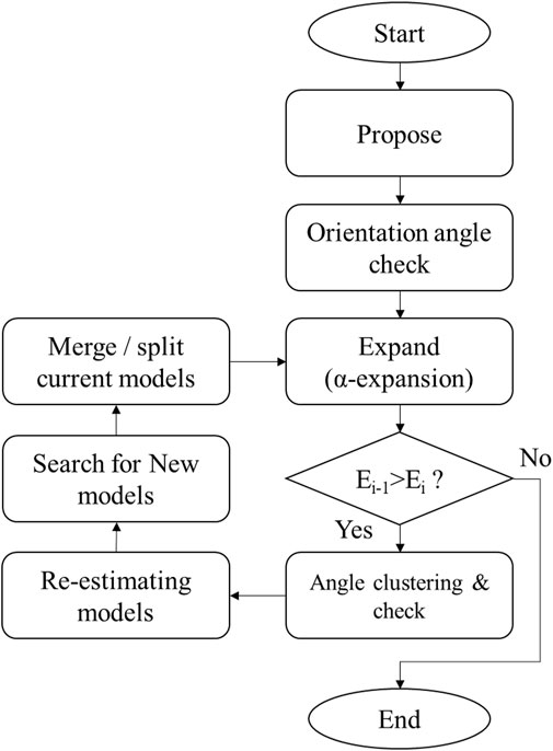
FIGURE 2. Schematic diagram of the GARNET algorithm.

1) Initial label sets ($L_{\mathit{0}}$) are generated from the given data by random sampling, using the maximum number of predefined models possible. The initial model generation should incorporate the maximum number of possible points. In this study, the RANSAC algorithm was used to rapidly generate the initial models and assign points to initial labels.

2) The orientations of the generated fracture model from label and those of the points assigned to the label are compared to eliminate insignificant data showing large angle-value differences. In this study, the angle was calculated using the difference between the normal vectors.

3) For energy minimization, $\alpha$-expansion is performed using Eq. 3. In this step, the spatially consistent label that includes the highest number of inliers is obtained through expansion between labels.

4) If energy minimization is not achieved in step 3), the final labels are output and calculate the errors between their normal vector angles of plane and point. Conversely, the iterative algorithm operation was continued.

5) When the energy decreases, DBSCAN is used to cluster the orientations of the points assigned to each label for classification. The cluster with the maximum number of points is extracted and then compared the orientations from the fracture model and the location points used in step 2) to eliminate data with large angle differences from the label.

6) The remaining labels are re-estimated and the existing label set is replaced with a new set satisfying Eq. 5.

7) New points associated with the fracture models are extracted from the points assigned to the outlier label.

8) If planes with similar model parameters are present, the difference between their normal vector angles and distances are calculated, and the fracture planes satisfying the conditions are merged. Then we return to Step 3) to restart from the $\alpha$-expansion for energy minimization.

3 Numerical experiments

A synthetic seismic dataset was applied to the fracture network imaging using the GARNET algorithm.

3.1 Orientation angle usability

The principal difference between the GARNET algorithm and the original PEARL algorithm is the incorporation of orientation data for accurate model imaging. Therefore, the effect of orientation on fracture imaging was examined using an identical point cloud. The synthetic data model was constructed to include six fracture planes in 80 m × 80 m × 150 m cubes and approximately 200 randomly distributed locations per plane, as shown in Figure 3. To reproduce the measurements and errors during data processing, a standard deviation (SD) of 2 was applied to the actual points to randomly alter their locations.

FIGURE 3

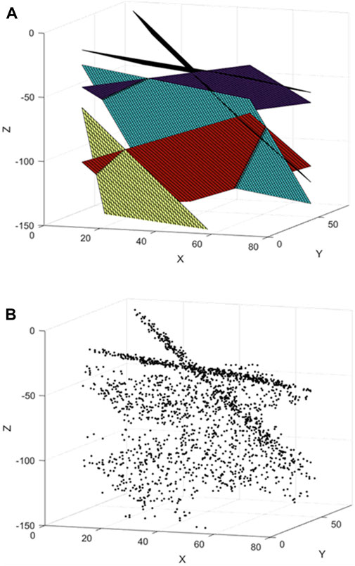
FIGURE 3. Synthetic experiments to verify the effect of orientation on fracture plane extraction. (A) True model consisting of six fracture planes and (B) 200 randomly distributed points from each fracture plane with low ratios of location errors.

First, the fractures were estimated using only points without orientations as the synthetic data. The initial model created using these points, with approximately 100 randomly generated planes, is shown in Figure 4A. Instead of using three points to generate numerous initial models, the RANSAC algorithm was used to promote the rapid assignment of points to labels. The value of threshold distance was 2 and each plane was generated using at least four points.

FIGURE 4

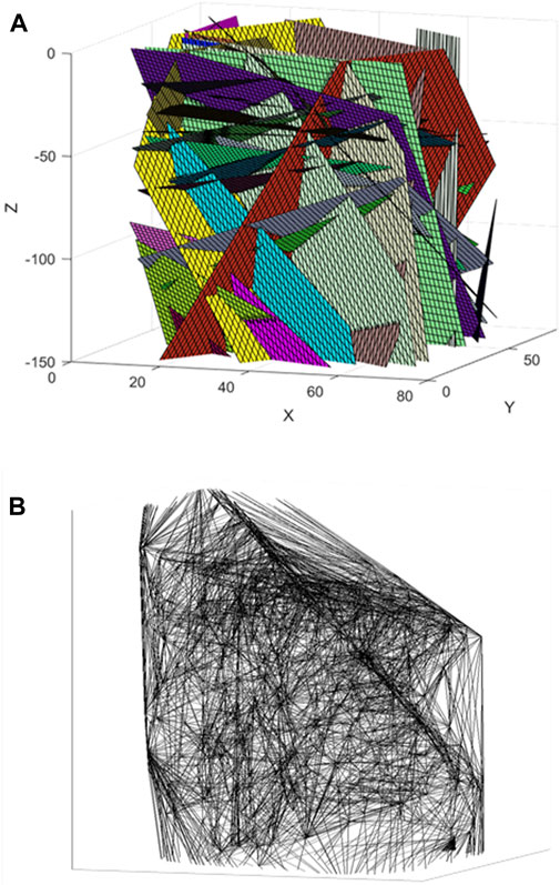
FIGURE 4. (A) Initial model created using the Random Sample Consensus (RANSAC) method with 100 randomly generated planes. (B) Results of Delaunay triangulation application to the synthetic data shown in Figure 3B.

To calculate the energy, the smoothing term in Eq. 1 requires clear information about the neighborhood from which the data are collected. In this study, the Delaunay triangulation method was used to reproduce the neighborhood system of the data, and the results are shown in Figure 4B. The first iteration of the re-estimated model is shown in Figure 5A. Compared with the initial model, the number of insignificant planes decreased significantly after the expansion and re-estimation steps, indicating that the points switched labels. Images of the fracture model created after the re-estimation step incorporating outlier labels are shown in Figure 5B. New models were also investigated using points that were excluded from the existing label during the algorithm operation, thereby producing several models that were added to the existing labels.

FIGURE 5

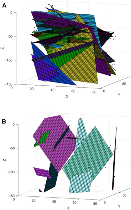
FIGURE 5. (A) Result of the re-estimated model in the first iteration without using orientation data. (B) New plane models for the outlier label after the re-estimation step.

The result of fracture modeling without orientation data are shown in Figure 6. Although convergence was achieved after only four iterations, 10 planes were estimated, demonstrating an overestimation compared to the actual fracture planes shown in Figure 3A. The estimated fracture orientations of many planes differ from the actual orientations. The errors associated with the strike and dip angle of plane estimates were 20.23% and 24.63%, respectively. If the actual fracture pattern is partially known, then it is safe to assume that statistical estimation is possible after multiple iterations, as long as the input parameters are adequately controlled. However, the accuracy of the orientations of the modeled fractures cannot be guaranteed.

FIGURE 6

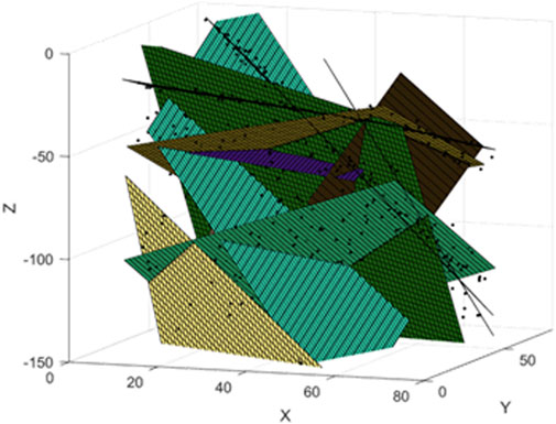
FIGURE 6. Result of fracture modeling without orientation data. The extracted planes were overestimated compared to the true model shown in Figure 3A.

Next, the fractures were modeled by integrating the orientation data with the location points as input data in the GARNET algorithm and applying these data to the synthetic model shown in Figure 3. After the initial model selection and energy calculation, the orientation clustering step was added to the estimation method, using only the location points. The results of eliminating models using orientation data with differences ≥30° between the plane orientation and the mean angle of the location points after the initial model was generated are shown in Figure 7A, confirming that the randomly generated initial model exhibited sorting consistent with the actual fracture pattern based solely on the selection process.

FIGURE 7

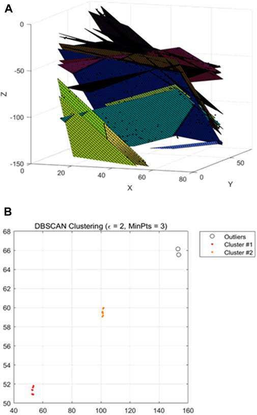
FIGURE 7. (A) Initial model removing planes with large angular differences between planes and locations. (B) Results of orientation clustering after energy reduction.

During subsequent energy calculations, orientation clustering was performed for each label if the energy decreased; the result confirmed the presence of clusters with different orientations within the same label (Figure 7B). This indicates that the application of energy optimization for distance can produce inaccurate fracture models. Therefore, the cluster with the most points was extracted and retained after clustering, whereas all other points were excluded from the label.

The result of fracture modeling using orientation data are presented in Figure 8. Convergence was achieved after only three iterations, and the number and orientation of the modeled fracture planes were consistent with those of the actual fracture model (Figure 3A). The errors of the plane shown in the result were 1.32% and 0.83% for the strike and dip, respectively. When the orientation data were missing, the number of iterations was lower and the computation time was reduced. These results confirm that fractures were modeled more rapidly and reliably using the GARNET algorithm involving the orientation data.

FIGURE 8

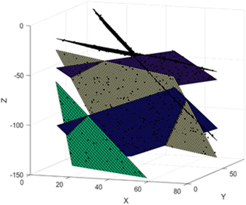
FIGURE 8. Result of fracture modeling using orientation data. The number and orientation of the planes were almost identical to those of the true model shown in Figure 3A.

3.2 Application to synthetic data including noise and outliers

The applicability of the GARNET algorithm was verified using a fracture model. In this subsection, we examine the suitability of the algorithm for modeling fractures when the locations cannot be accurately expressed owing to the presence of many errors and outliers unrelated to fractures in the acquired data. The synthetic data model comprises 10 fracture planes (Figure 9A), with each plane containing approximately 100 randomly distributed points. To reproduce data with many errors, SD values of 6 and ≥12 were applied to the location and orientation data, respectively, to randomly alter both parameters. In addition, 500 outlier points that were unrelated to the microseismic event were randomly generated (Figure 9B).

FIGURE 9

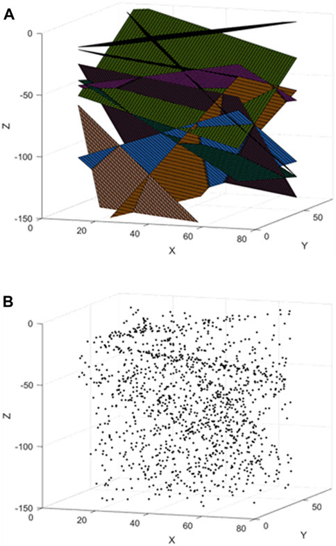
FIGURE 9. Synthetic experiments to verify the suitability of the GARNET algorithm for location data including outliers. (A) True model consisting of 10 fracture planes, (B) 100 randomly distributed points from each fracture plane with high ratios of location errors and 500 outlier points independent of the microseismic event.

The results of the DBSCAN analysis performed on the orientation of the points assigned to the labels during the first iteration (Figure 10A) indicate that for fractures associated with a complex formation process, the probability of points assigned to the labels belonging to multiple clusters with diverse orientations and many outliers is high. The results of the model re-estimation performed after orientation clustering for the same number of iterations are shown in Figure 10B. Although not all fracture planes were identified, a pattern similar to that of the actual planes emerged, despite many outliers. The results of the fracture modeling using data, including noise and outliers, are presented in Figure 11A. The number and orientation of the modeled fracture planes were not significantly different from those of the actual fracture model (Figure 9A). The errors of the strike and dip angle estimates were 1.89% and 1.64%, respectively.

FIGURE 10

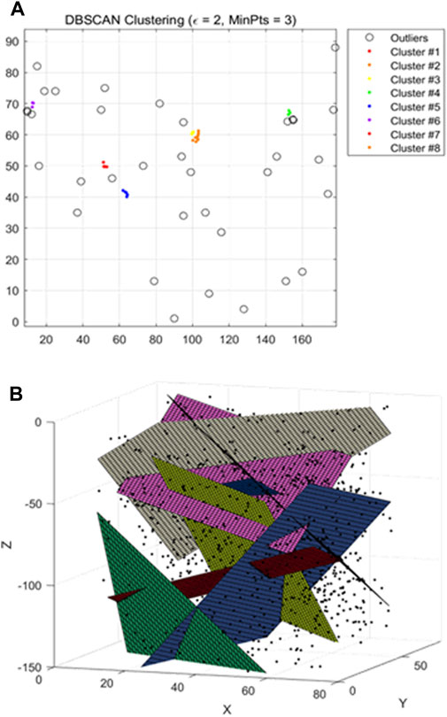
FIGURE 10. (A) Result of orientation clustering using the density-based spatial clustering of applications with noise (DBSCAN) method in the first iteration. Events associated with labels were classified as orientation clusters and outliers. (B) Result of the re-estimated model in the first iteration. Extracted planes were similar to those of the true model from among data with many outliers.

FIGURE 11

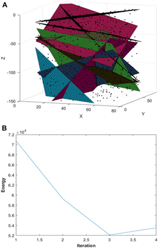
FIGURE 11. (A) Result of fracture modeling using the GARNET algorithm for data containing high noise levels and many outliers. (B) Energy values obtained after each iteration were minimized in the third iteration.

The energy decreased rapidly during the iteration, and the optimal fracture model planes were estimated through energy minimization within three iterations (Figure 11B). These synthesis model results confirmed that the fracture models were robustly estimated using the proposed GARNET algorithm, despite the inclusion of many location measurement errors or outliers in the data.

4 Application to field microseismic data

To investigate the applicability of the developed algorithm to field microseismic data, it was utilized data acquired during the Geysers Enhanced Geothermal System (EGS) resource development project in California, USA as shown in Figure 12A. This project was conducted to enhance the technology for assessing the temporal changes and volumetric distribution of fluids introduced during resource development, as well as field stress magnitudes, fracture sizes, and orientations. Using a network comprising 34 permanent geophones, high-frequency seismic data were acquired as broadband data using a temporary network containing 33 geophones. The analysis of the acquired data revealed 752 microseismic events (Gritto et al., 2018), as shown in Figure 12B.

FIGURE 12

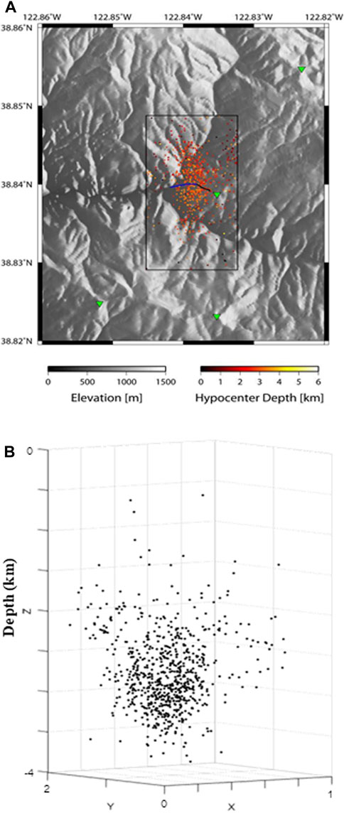
FIGURE 12. (A) Microseismic events detected by The Geysers broadband and geophone network in the vicinity near the injection site, adapted from Gritto et al. (2018). (B) Microseismic data were monitored by 34 permanent and 33 temporary geophones; 752 microseismic events were evaluated.

During the fracture network modeling, orientation clustering was performed for each label by applying the GARNET algorithm to the field data. The ε and MinPts values were 2 and 3, respectively, and the result of fracture network produced is shown in Figure 13A. The angle of the normal vector for convergence was set to 15°, and the fracture planes were obtained via energy convergence after only three iterations. The estimated number of fracture planes was 6, and the errors associated with the strike and dip angle estimates were 2.89% and 2.83%, respectively. All fracture planes produced strike values of N10°E-N30°E and a dip of 75°–85°, with no overlapping orientation. The statistical representation result of the fracture network using the same microseismic event data are presented in Figure 13B (Gritto et al., 2018). The rupture area is shown by the size of the circle; the colored points at the hypocenters represent the moment magnitude of the event. The estimated orientation of the rupture area is almost similar to the orientation estimated by GARNET with a strike of N10°E±10° and a dip of 80°±10°.

FIGURE 13

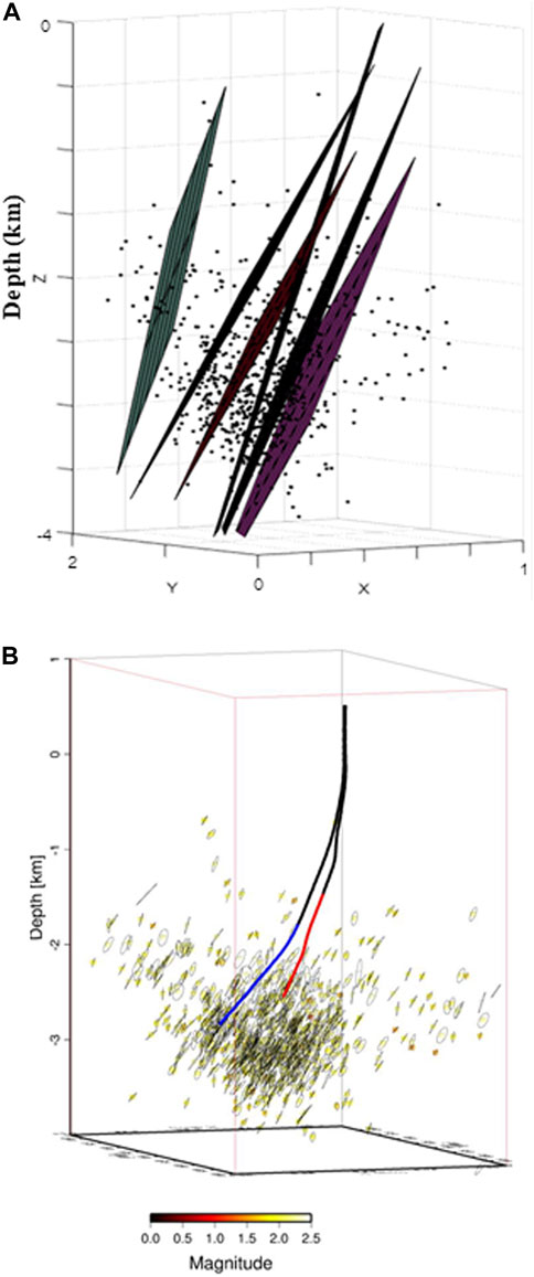
FIGURE 13. (A) Fracture network imaging results obtained using the GARNET algorithm with microseismic location and orientation data. (B) Statistical representation of the generated fracture network below production well (red) and injection well (blue), adapted from Gritto et al. (2018).

These results demonstrate that the fractures progressed along a particular orientation owing to hydraulic fracturing in the boreholes. Because data with inconsistent orientations or insufficient points are eliminated by orientation clustering, network modeling is simpler. These results confirm the suitability of the algorithm for orientation and location data in the rapid and accurate modeling of field data involving major fracture plane networks.

5 Conclusion

The GARNET algorithm was developed as an improved version of the PEARL algorithm, and then used for fracture network imaging. The GARNET algorithm exploits the location data acquired during microseismic events or earthquakes, and orientation data obtained from the moment tensors of associated events. The function of this algorithm improves the location accuracy of the estimated fracture plane by generating and reproducing labels based on the energy differences between locations. In addition, clustering using DBSCAN was applied to the orientation angle to improve the reliability of the extracted fracture direction.

Synthetic data suitable for simulating microseismic events were used to assess the performance of the algorithm. A synthetic fracture model relying solely on location data exhibited poor accuracy in estimating the number and orientation of the fracture planes. Conversely, the number and orientation of the fracture planes obtained using the proposed algorithm incorporating orientation data matched those in the actual data. In the second synthetic model, fractures were modeled by applying the algorithm to data with high noise levels and many outliers. The results demonstrated robust fracture plane estimation with a negligible impact of errors and outliers, despite few iterations. The proposed algorithm was also applied to field data acquired during an EGS resource development project to assess its utility. The resulting fracture network modeling process produced strike orientations of N10°E–N30°E and a dip angle of 75°–85°, with six representative fracture planes. The errors associated with the strike and dip angle estimates were 2.89% and 2.83%, respectively. These results are similar to statistical representation results, and we validated the suitability of the algorithm for accurately simulating fracture locations and orientations in real fracture networks.

Data availability statement

The datasets presented in this study can be found in online repositories. The names of the repository/repositories and accession number(s) can be found below: The field data were obtained through work supported by the Department of Energy’s Office of Energy Efficiency and Renewable Energy (EERE) in association with the Geothermal Technologies Office (GTO) and can be found in the Geothermal Data Repository (https://gdr.openei.org/).

Author contributions

JY wrote the article and developed the code. YJ conceptualized the modeling methods and analyzed the applied techniques. BK provided field data information and data processing expertise.

Funding

This work was supported by a basic research project of the Korea Institute of Geoscience and Mineral Resources (GP 2020–023) funded by the Ministry of Science and ICT of Korea.

Acknowledgments

The authors would like to thank the reviewers for their valuable and careful comments.

Conflict of interest

The authors declare that the research was conducted in the absence of any commercial or financial relationships that could be construed as a potential conflict of interest.

Publisher’s note

All claims expressed in this article are solely those of the authors and do not necessarily represent those of their affiliated organizations, or those of the publisher, the editors and the reviewers. Any product that may be evaluated in this article, or claim that may be made by its manufacturer, is not guaranteed or endorsed by the publisher.

References

Aki, K., and Richards, P. G. (2009). Quantitative seismology. Sausalito: University Science Books, Cop.

Google Scholar

Boykov, Y., Veksler, O., and Zabih, R. (2001). Fast approximate energy minimization via graph cuts. IEEE Trans. Pattern Anal. Mach. Intell. 23 (11), 1222–1239. doi:10.1109/34.969114

CrossRef Full Text | Google Scholar

Busetti, S., Jiao, W., and Reches, Z. (2014). Geomechanics of hydrolic fracturing microseismicity: Part 2. Stress state determination. Am. Assoc. Pet. Geol. Bull. 98, 2459–2476. doi:10.1306/05141413124

CrossRef Full Text | Google Scholar

Chebi, H., Acheli, D., and Kesraoui, M. (2016). Dynamic detection of abnormalities in video analysis of crowd behavior with DBSCAN and neural networks. Adv. Sci. Technol. Eng. Syst. J. 1, 56–63. doi:10.25046/aj010510

CrossRef Full Text | Google Scholar

Delong, A., Osokin, A., Isack, H., and Boykov, Y. (2012). Fast approximate energy minimization with label costs. Int. J. Comput. Vis. 96 (1), 1–27. doi:10.1007/s11263-011-0437-z

CrossRef Full Text | Google Scholar

Dershowitz, W. S., and Fidelibus, C. (1999). Derivation of equivalent pipe network analogues for three-dimensional discrete fracture networks by the boundary element method. Water Resour. Res. 35 (9), 2685–2691. doi:10.1029/1999wr900118

CrossRef Full Text | Google Scholar

Duda, R. O., and Hart, P. E. (1972). Use of the Hough transformation to detect lines and curves in pictures. Commun. ACM 15 (1), 11–15. doi:10.1145/361237.361242

CrossRef Full Text | Google Scholar

Economides, M. J., and Nolte, K. G. (2000). Reservoir stimulation. Chichester: Wiley.

Google Scholar

Ester, M., Kriegel, H.-P., Sander, J., and Xu, X. (1996). A density-based algorithm for discovering clusters in large spatial databases with noise. Kdd 96, 226–231.

Google Scholar

Fadakar Alghalandis, Y., Dowd, P. A., and Xu, C. (2013). The RANSAC method for generating fracture networks from micro-seismic event data. Math. Geosci. 45 (2), 207–224. doi:10.1007/s11004-012-9439-9

CrossRef Full Text | Google Scholar

Fischler, M. A., and Bolles, R. C. (1981). Random sample consensus: A paradigm for model fitting with applications to image analysis and automated cartography. Commun. ACM 24 (6), 381–395. doi:10.1145/358669.358692

CrossRef Full Text | Google Scholar

Fisher, N. I. (2005). Statistical analysis of circular data. Cambridge: Cambridge University.

Google Scholar

Gritto, R., Boyd, O. S., and Dreger, D. S. (2018). Seismic analysis of spatio-temporal fracture generation during EGS resource development-deviatoric MT, fracture network, and final report. United States: USDOE Geothermal Data Repository. doi:10.15121/1494306

CrossRef Full Text | Google Scholar

Gudmundsson, A. (2011). Rock fractures in geological processes. Cambridge: Cambridge University Press.

Google Scholar

Guo, Z., Liu, H., Pang, L., Fang, L., and Dou, W. (2020). DBSCAN-based point cloud extraction for Tomographic synthetic aperture radar (TomoSAR) three-dimensional (3D) building reconstruction. Int. J. Remote Sens. 42 (6), 2327–2349. doi:10.1080/01431161.2020.1851062

CrossRef Full Text | Google Scholar

Hyman, J. D., Karra, S., Makedonska, N., Gable, C. W., Painter, S. L., and Viswanathan, H. S. (2015). dfnWorks: A discrete fracture network framework for modeling subsurface flow and transport. Comput. Geosci. 84, 10–19. doi:10.1016/j.cageo.2015.08.001

CrossRef Full Text | Google Scholar

Isack, H., and Boykov, Y. (2011). Energy-based geometric multi-model fitting. Int. J. Comput. Vis. 97 (2), 123–147. doi:10.1007/s11263-011-0474-7

CrossRef Full Text | Google Scholar

Kwicklis, E. M., and Healy, R. W. (1993). Numerical investigation of steady liquid water flow in a variably saturated fracture network. Water Resour. Res. 29 (12), 4091–4102. doi:10.1029/93wr02348

CrossRef Full Text | Google Scholar

Li, L., and Lee, S. H. (2008). Efficient field-scale simulation of black oil in a naturally fractured reservoir through discrete fracture networks and homogenized media. SPE Reserv. Eval. Eng. 11, 750–758. doi:10.2118/103901-pa

CrossRef Full Text | Google Scholar

Liu, Y., Song, B., Wang, L., Gao, J., and Xu, R. (2020). Power transformer fault diagnosis based on dissolved gas analysis by correlation coefficient-DBSCAN. Appl. Sci. (Basel). 10 (13), 4440. doi:10.3390/app10134440

CrossRef Full Text | Google Scholar

Mardia, K. V., and Jupp, P. E. (2009). Directional statistics. Chichester: John Wiley & Sons.

Google Scholar

Mayer, J. R., and Sharp, J. M. (1998). Fracture control of regional ground-water flow in a carbonate aquifer in a semi-arid region. Geol. Soc. Am. Bull. 110 (2), 269–283. doi:10.1130/0016-7606(1998)110<0269:fcorgw>2.3.co;2

CrossRef Full Text | Google Scholar

Mitcham, T. W. (1963). Fractures, joints, faults, and fissures. Econ. Geol. 58 (7), 1157–1158. doi:10.2113/gsecongeo.58.7.1157

CrossRef Full Text | Google Scholar

Montgomery, C. T., and Smith, M. B. (2010). Hydraulic fracturing: History of an enduring technology. J. Petroleum Technol. 62 (12), 26–40. doi:10.2118/1210-0026-JPT

CrossRef Full Text | Google Scholar

Raven, K. G., and Gale, J. E. (1985). Water flow in a natural rock fracture as a function of stress and sample size. Int. J. Rock Mech. Min. Sci. Geomechanics Abstr. 22 (4), 251–261. doi:10.1016/0148-9062(85)92952-3

CrossRef Full Text | Google Scholar

Valko, P., and Economides, M. J. (2001). Hydraulic fracture mechanics. Chichester: John Wiley & Sons.

Google Scholar

Warpinski, N. R., Mayerhofer, M., Agarwal, K., and Du, J. (2013). Hydraulic-fracture geomechanics and microseismic-source mechanisms. SPE J. 18, 766–780. doi:10.2118/158935-pa

CrossRef Full Text | Google Scholar

Yu, J., Byun, J., and Seol, S. J. (2020). Imaging discrete fracture networks using the location and moment tensors of microseismic events. Explor. Geophys. 52 (1), 42–53. doi:10.1080/08123985.2020.1761760

CrossRef Full Text | Google Scholar

Yu, X., Rutledge, J., Leaney, S., and Maxwell, S. (2016). Discrete-fracture-network generation from microseismic data by use of moment-tensor- and event-location-constrained Hough transforms. SPE J. 21 (1), 221–232. doi:10.2118/168582-pa

CrossRef Full Text | Google Scholar

Zhang, H., Nadeau, R. M., and Toksoz, M. N. (2010). Locating nonvolcanic tremors beneath the San Andreas Fault using a station-pair double-difference location method. Geophys. Res. Lett. 37 (13), L13304. doi:10.1029/2010gl043577

CrossRef Full Text | Google Scholar