Deformation monitoring and influence factor analysis of expressway over strong saline soil based on an advanced multi-temporal InSAR technique

Saline soil harbors crystallized salt in the solid phase and salt solution in the liquid phase. By the natural environmental and human activity factors, migration and accumulation of the salt and crystallization process alternated with dissolving, which makes saline soil with significant seasonal differences appear in the deformation and regional scattering characteristic. These phenomena raise the limitation of conventional multi-temporal interferometric synthetic aperture radar (MT-InSAR) technique and consequently high-precision deformation monitoring of strong saline soil subgrade and pavement. To overcome the limitations, this study aimed to propose an advanced MT-InSAR method, which considers the seasonal interferometric coherences caused by precipitation and the temporal physical deformation evolution of the subgrade and pavement over strong saline soil. To present the better performance of the advanced method, a segment of the Qarhan–Golmud Expressway (QGE), which is the first expressway built in the strong saline soil area in China, was selected for this study. Two sets of SAR images acquired from January 2018 to January 2022 from Sentinel-1A ascending and descending orbits over the QGE were utilized, 774 and 928 seasonal filtered interferograms are optimized for deformation monitoring based on the deformation Poisson curve (PC) model. Compared with the method in the previous studies, the accuracy, efficiency, and reliability of the monitoring results increased dramatically. Subsequently, further discussions are conducted in detail on the regularity of expressway deformation over strong saline soil, especially from physical and chemical perspectives. Findings show that the ratio between Cl⁻ and SO₄^2- determines the deformation distribution and morphology. Also, the precipitation and temperature affect the seasonal characteristics. The contributions of this investigation might provide technical references for related expressway management and policy-making departments to ensure the long-term safe operation and stability of the QGE.

1 Introduction

Due to the high environmental sensitivity, the engineering properties of saline soil can be easily affected by water, temperature, human activities, and other factors. The chemical reactions between salts and set cement and the effect of cyclic freeze–thaw on the water and salt migration can lead to subgrade and pavement diseases such as settlement, uplift, and fracture (Stipho, 1985; Shao, 2012). Hence, in a strong saline soil area, the subgrade construction of the expressway makes it necessary to take measures. Generally, saline soil can be tamped and compacted by dynamic consolidation and piling, and cut-off layers explored to prevent contact between capillary water, salt, and set cement. Moreover, drainage facilities are set to avoid precipitation immersion. After the opening of expressway, the precipitation, seasonal meltwater, temperature, heavy traffic, massive brine extraction, injection of freshwater, and other factors would bring negative forces to the porous construction materials. The durability of the aforementioned measures would be strongly affected. As time goes by, the salt migration and chemical reactions triggered seriously again, accompanied by accumulation of the salt and crystallization process alternated with dissolving, which makes the typical changes of saline soil’s physical and mechanical properties, such as strength, particle composition, salt content, salt type, and water content. Then, the complex deformation of the subgrade and pavement was created to affect the safety of expressway operation. Consequently, the cyclic damages caused by the complex deformation should be interpreted (Brouchkov, 2003; Castellazzi et al., 2013; Zhang et al., 2018a). Numerous previous studies have experimented discretely under an ideal environment to further analyze the interplay of these internal and external factors based on saline soil typical sample selection and variable controlling in the indoor laboratory (Wu and Zhu, 2002; Wang et al., 2016; Zhang et al., 2018b). Nevertheless, the actual outdoor environment changes rapidly, and traditional engineering monitoring methods, field investigation, and geotechnical analysis are limited by sparse instrumentation, low spatiotemporal resolution, high cost, etc. Large-scale continuous deformation monitoring of subgrade and pavement on the strong saline soil in the field environment is barely contributed.

MT-InSAR technology provides an excellent monitoring tool to evaluate the stability of the expressway by providing millimeter precision deformation measurements with bi-weekly or monthly updates. It has large and continuous spatial coverage and is not affected by clouds and rains. The main methodologies including persistent scatter-InSAR^TM (PS-InSAR^TM), Stacking-DInSAR, and small baseline subset (SBAS)-InSAR were remodified and advanced for all kinds of complicated earth observations (Massonnet et al., 1993; Ferretti et al., 2000; Liu et al., 2000; Berardino et al., 2002; Jianjun et al., 2017; Dai et al., 2020; Cui et al., 2021; Li et al., 2022). Indeed, few studies considered the seasonal factors in the MT-InSAR technology to obtain the deformation of infrastructures in the strong saline soil areas. These studies set a relatively large temporal baseline threshold initially for seeking enough candidate interferograms. Then, the average interferometric coherence coefficients of thousands of interferograms are calculated for further analysis. After that, they find that the interferometric coherences are highly correlated with the precipitation. Finally, the interferograms with average spatial coherence higher than 0.5 are refined as the available interferograms (Hu et al., 2017; Rui et al., 2021; Xiang et al., 2021; Xiang et al., 2022). Such heavy computation requirements are not suitable for long-term monitoring.

Hence, it is necessary to sum up the rules for refining the interferogram network directly while guaranteeing enough redundant observations. On this basis, reliable distributed targets (DTs) can be selected for deformation estimation. However, the traditional InSAR deformation models are hard to describe the temporal physical deformation evolution of the subgrade and pavement over strong saline soil with better reality (Zhang et al., 2012; Li et al., 2013; Liao and Wang, 2014). To solve this problem, the Poisson curve can be joined into the deformation model, which has been widely used in the field of highway post-construction prediction (Zhu and Zhou, 2009). Under this conception, a 32.25 km segment across the Qarhan Salt Lake (QSL) of the QGE is selected as the study target. We used an advanced MT-InSAR method to extract the deformation of subgrade and pavement over strong saline soil based on the interferogram seasonal filtering and the Poisson curve. Subsequently, based on the analysis of the chemical reactions between the salts and concrete, we discussed the deformation rules of the study segment along the QGE piecewise. Finally, we suspect the ratio between Cl⁻ and SO₄^2- (Cl⁻/SO₄^2-) determines the deformation distribution and morphology, and the precipitation and temperature affect the seasonal characteristics. This study helped to provide a reliable basis for related departments of transportation management in road maintenance.

2 Natural geography background of study area and data sources

As the final traffic hinge of the G3011 (Liuyuan–Golmud Expressway, LGE), the QGE (37°06′47″–36°21′56″ N and 95°27′36″–95°02′45″ E) is the first expressway which was built in the strong saline soil area of China. It is located in the eastern Qaidam Basin, a triangle region that consists of Aerjin Mountain, Qilian Mountain, and Kunlun Mountain fault fold belt (Wei et al., 2016). The segment with poor geological conditions (the yellow and black lines in Figure 1) is from K585+000 to K617+250, which crosses the QSL and belongs to the cold region of Qinghai–Tibet Plateau (QTP) in the Chinese expressway natural regionalization. This area is selected for our study with elevations ranging from 2680 m to 3200 m. It is a flat lacustrine plain with more than 1 km thick quaternary and several E-W and NW-SE faults (Zhang et al., 2018a). Due to the surroundings of high mountains, it is hard for the southwest warm moist air to enter in. Naturally, the weather is dry, rainless, with uneven precipitation, and windy all the year. In recent 4 years, the meteorological data of Golmud station are shown in Figure 2, the local monthly mean precipitation is 0–30 mm, mostly coming from June to September. The highest and lowest monthly mean temperatures are 23°C and 16.1°C, respectively. The temperature difference between day and night is obvious, and the annual evaporation is more than 2500 mm because of abundant solar radiation, heat, and strong winds (Shao, 2012). Meanwhile, the rainfall and melt-water from the surrounding mountains provide minerals and water sources for the basin.

FIGURE 1

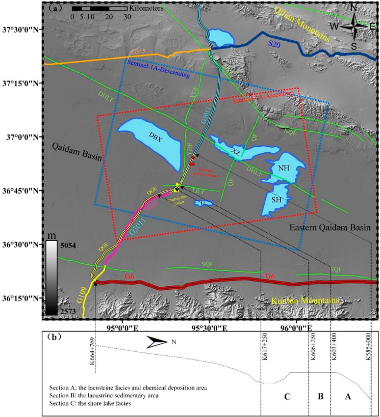
FIGURE 1. (A) Tectonic map of the study area. The blue and black, red and black, and yellow and black lines indicate the G3011 (Liuyuan–Golmud Expressway, LGE), the G6 (Beijing–Tibet Expressway, BTE), and the QGE (Qarhan–Golmud Expressway), respectively. The yellow, purple, and brown lines denote the G109, G215, and G315, respectively. The blue and red rectangles mark the coverage of the descending and ascending Sentinel-1A images. The blue polygons represent the DBX (Dabuxun lake), XZ (Xiezuo lake), TJ (Tuanjie lake), NH (North Huobuxun lake), and SH (South Huobuxun lake), respectively. The green lines denote the faults in this area, including NQF (North Qaidam Fault), SQF (South Qaidam Fault), TJLK (Tuanjian Lake Fault), QF (Qarhan Fault), YDF (Yaxi–Dadong Fault), and DHLF (Dabuxun–Huobuxun Lake Fault). The red and yellow flags indicate the Dabuxun Railway Station (DRS) and Qarhan Bus Station (QBS). (B) General layout of the QGE. A, B, and C represent three different depositional areas.

FIGURE 2

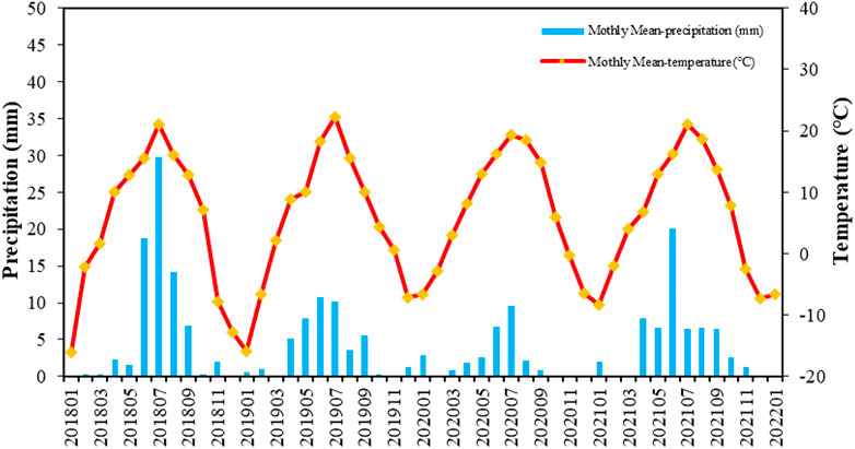
FIGURE 2. Monthly mean temperature and precipitation data of the Golmud station (36.417° N and 94.9° E) from January 2018 to January 2022.

Under the intense evaporation, the water of QSL is dwindling with salinity increasing and salt constantly precipitation. In the QSL region, only three lakes are filled with water all year round, North Huobuxun (NH), South Huobuxun (SH), and Dabuxun (DBX), respectively. Tuanjie (TJ) and Xiezuo (XZ) are seasonal lakes (Wei et al., 2016). Along the study segment of QGE, the surface is covered with a thickness of 0.2 m–0.6 m salt crust, and rich brine with chlorine salt type and strong saline distribute widely. For piecewise analysis, we divided the study segment into three parts according to the differences in sediment traps (Figure 1B), including the lacustrine facies and chemical sedimentary area (the chainage is from K585+000 to K603+400, segment A), the lacustrine facies sedimentary area (the chainage is from K603+400 to K606+250, segment B), and the shore lake facies sedimentary area (the chainage is from K606+250 to K617+250, segment C).

The engineering geological properties of the study segment are poor due to the dramatic change in saline soil compositions and pore structures. The deformation of subgrade and pavement in these kinds of areas is foreseeable. In the circumstances, a set of 110 ascending and 115 descending images of Sentinel-1A (2018–2022) from the European Space Agency (ESA) with a resolution of about 2.33 m × 13.97 m (range × azimuth) is used in our study (Table 1). The 30-m high-resolution digital elevation model (DEM) is provided by the National Aeronautics and Space Administration (NASA). The precise orbit data (POD) of images are provided by the ESA.

TABLE 1

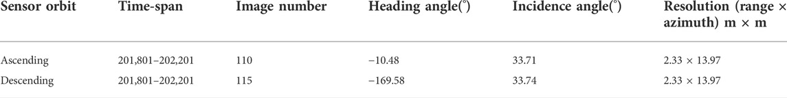
TABLE 1. Sentinel-1A datasets and primary image parameters.

3 Materials and methods

In these similar saline mudflat areas, 90% of the ground coverage is distributed targets (DTs), such as roads, deserts, bare lands, and human-made structures. They occupy tens of pixels in SAR images and keep stable with moderate coherence values in time series (Li, 2014). To obtain DTs maximally, a typical and mature MT-InSAR method termed the SBAS-InSAR detects deformation by using interferometric pairs with short spatial baselines (Berardino et al., 2002; Li, 2014). As a consequence, the network connection restricts the monitoring precision crucially. Since the saline soil has high environmental sensitivity. Some extreme environmental factors, especially seasonal variations may bring spatiotemporal decoherence to the DTs. To improve the monitoring precision and efficiencies, we optimized the conventional SBAS-InSAR by considering the precipitation. Concretely, interferogram networking, interferogram seasonal filtering, interferogram network rebuilding and inversion, and distributed target (DT) selection comprise the procedures shown in Figure 3.

FIGURE 3

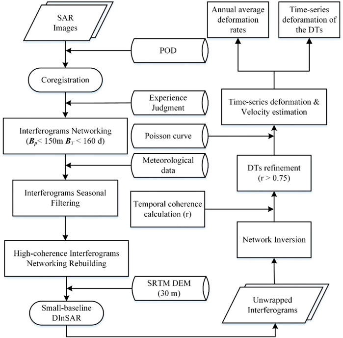
FIGURE 3. Work-flow of the optimized MT-InSAR.

3.1 Interferogram seasonal filtering and high-coherence interferogram networking rebuilding

The previous studies found that the interferometric coherence coefficients in these similar saline mudflat areas have seasonal changes. As shown in Figure 4 (by setting the temporal baseline threshold for 400 days that includes a whole year and the perpendicular spatial baseline threshold for 200 m, a total of 2,921 interferograms are formed with 119 Sentinel-1A images acquired from 2015 to 2020) (Xiang et al., 2021), in the rainy season, the high interferometric coherences of interferograms mainly occur between June and November and disappear dramatically after November. But in the dry season, the high coherences appear again between November and the next April or May. This result proves that the interferometric coherences decrease dramatically due to the increase in precipitation from the dry season to the rainy season (Rui et al., 2021; Xiang et al., 2021; Xiang et al., 2022). However, thousands of average interferometric coherence coefficients are needed for the calculation for further analysis; such a heavy computation requirement is not suitable for long-term monitoring.

FIGURE 4

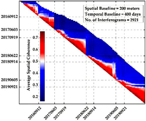
FIGURE 4. Average interferometric coherence coefficients from 2015 to 2020, the vertical axis represents the period of the primary images and the horizontal axis represents the period of the secondary images. The color values of pixels represent the ASC of the interferograms (Xiang et al., 2021).

Hence, we sum up the rules for refining the interferogram network directly while guaranteeing enough redundant observations. There are two steps of interferogram seasonal filtering. In the first step of interferogram seasonal filtering: we set a temporal baseline B_T of 160 days after considering the key time range of precipitation changes. Meanwhile, we set a perpendicular baseline of 150 m strictly to maintain the high quality of interferograms. The initial ascending and descending networks are formed by 1,144 and 1,277 interferograms, respectively. Such a calculated amount is still intractable for computing efficiency. Hence, the second step of interferogram seasonal filtering needs to be critical to reducing the interferograms while maintaining enough high-quality beneficial redundant observations. As for these similar saline mudflat areas, the instantaneous intense rainfall may bring noticeable differences to interferogram coherence. On a monthly scale, there is no reference value of little rain because of high evaporation. Therefore, we took 5 mm, 15 mm, and 25 mm of monthly precipitation as the lowest standard value of the normal, middle, and supernormal valid precipitation for comprehensive consideration.

As shown in Figure 2, the monthly mean precipitation concentrates in the period from April to September. We count the number of the normal, middle, and supernormal valid precipitation by treating one-time normal precipitation as the counting unit (CU). Moreover, the middle and supernormal represent three times and five times normal precipitation, respectively. The detailed counting information of our study years is shown in Table 2. After combining Figure 2 and table 2, we found that the middle precipitation appears once in 2018 (June) and 2021 (June), and the supernormal precipitation appears once in 2018 (July). In addition, the normal precipitation continues from April to September in 2019 and 2021. But in 2020, the normal precipitation appears only two times between June and July. The CUs of these 4 years are 10, 10, 2, and 11, respectively. We set the CUs of 5 as the boundary to separate the dry and rainy years, consequently, 2018, 2019, and 2021 are the rainy years while 2020 is the dry year.

TABLE 2

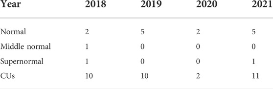
TABLE 2. Number of normal and supernormal valid precipitation.

Based on these data, we filtered the interferogram network of the dry and rainy years directly through three conditional judgments as follows:

1) Dry year (January to December).

The network remains the initial form if there are no connections with the normal precipitation month. If not, the whole connections will be filtered.

2) Rainy year (January to May, and October to December).

The network remains in the initial form if there are no connections with the months from June to September. If not, the whole connections will be filtered.

3) Rainy year (January to September).

The network remains in the initial form if there are no connections with the months from June to September. If not, the whole connection will be filtered. After June or July, we filter the needless connections and remain 4 or 6 connections nearby only until September over, depending on whether the period has the middle or supernormal precipitation months, 4 is yes, and 6 is no.

As shown in Figure 5, after two times of interferogram seasonal filtering, the rebuilding ascending and descending networks are formed by 774 and 927 interferograms, respectively. The number of interferograms is reduced by about 360 interferograms compared with the initial network; as a result, the computing efficiency improves obviously.

FIGURE 5

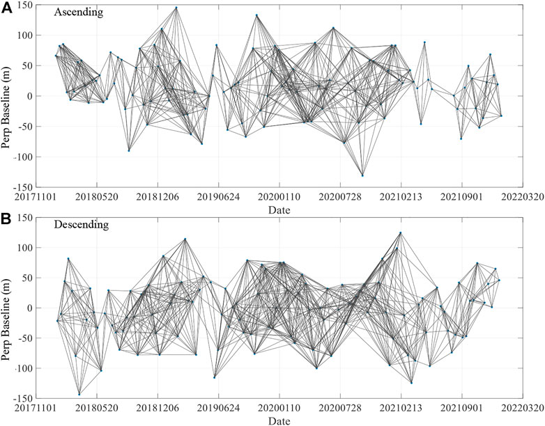
FIGURE 5. High-coherence interferogram rebuilding network after seasonal filtering. (A) and (B) indicate the network of ascending and descending interferograms.

3.2 The deformation extraction of the study area

For the conventional MT-InSAR (PS-InSAR^TM and SBAS-InSAR), it is hard to obtain the DTs maximally in the study area. Because of the interferograms, coherence seasonal characteristics are affected by kinds of external environmental factors such as precipitation and temperature, we performed interferogram seasonal filtering to optimize the network and select the DTs through a strict temporal coherence threshold (0.75) based on the conventional SBAS-InSAR (Rui et al., 2021; Xiang et al., 2021; Xiang et al., 2022). Whereafter, the time series deformation model based on the Poisson curve (PC) is applied to obtain high-precision time series deformation results of the DTs (Ming-hua et al., 2005; Zhu and Zhou, 2009; Yang et al., 2016; Jianjun et al., 2017; Zhu et al., 2021).

In the conventional SBAS-InSAR processing, sets of repeat-pass SAR images in a certain period (t₀, … , t_n) are collected first. Then the registration of all the images can be processed in the same coordinate system. Also, certain spatial and temporal thresholds can be set to obtain high-quality interferometric pairs based on the differential InSAR (DInSAR) method. The phase unwrapping and removing of the topographic phase for each interferometric pair can be executed subsequently. The unwrapped phase at pixel (x, y) in the ith interferogram with the period from t_A to t_B (t_B > t_A) can be expressed as (Berardino et al., 2002)

$\delta {\phi }_i\left(x, y\right)={\phi }_B\left(x, y\right)-{\phi }_A\left(x,y\right)\approx \frac{4\pi }{\lambda }\left[d\left(t_B,x,y\right)-d\left(t_A,x,y\right)\right]+\mathrm{\Delta }{\phi }_{topo}^i\left(x,y\right)+\mathrm{\Delta }{\phi }_{res}^i\left(x,y\right),(1)$

where λ is the wavelength (0.056 m for C-band Sentinel-1A data), i $\in$ (1, … , M) denotes the index of interferograms, and d (t_B, x, y) and d (t_A, x, and y) imply the cumulative LOS (line of sight) displacement at dates t_B and t_A with respect to d (t₀, x, y) = 0, respectively. $\mathrm{\Delta }{\phi }_{topo}^i\left(x,y\right)= \frac{4\pi B_{\perp }}{\text{λ}R\text{sin}\theta }\mathrm{\Delta }h\left(x,y\right)$, R is the range between the sensor and ground object, B_⊥ defines the spatial baseline, $\theta$ is the incidence angle, $\mathrm{\Delta }h$ represents the elevation correction, and $\mathrm{\Delta }{\phi }_{res}^i\left(x,y\right)$ defines the residual phase component, which is related to noise, atmospheric delay, and high-pass (HP) deformation.

In the linear deformation model, a linear variation is assumed to the displacement for each time-adjacent interferometric period. The functional relationship can be written as

$d\left(t_B,x,y\right)-d\left(t_A,x,y\right)=v_i\cdot \left(t_B-t_A\right),(2)$

where $v_i$ stands for the linear velocity for each temporal unit, and it varies in different temporal units. We substitute Equation 2 into Equation 1, the linear velocities in different periods and the elevation correction become the rest of the unknown parameters. It is a typical least square (LS) problem. In allusion to the singularity of the equation coefficient matrix, we utilized the singular value decomposition method to estimate the linear rate for each period (Jianjun et al., 2017). By integrating the velocity of each period, the final linear time series deformation can be extracted.

Considering the seasonal characteristics of deformation in the study area (strong saline soil area), we unitized a time series deformation model based on the Poisson curve (PC) to reflect the varying disciplines. The PC is a typical “S” type growth curve, it is widely applied to the deformation prediction of subgrade and pavement (Zhu and Zhou, 2009). The PC can be expressed as

$W\left(t\right)=\frac{W_0}{1+a{e}^{-bt}}=d_{LOS}\left(t\right),(3)$

where W(t) is the dynamic ground subsidence at time t with respect to the reference time t₀ = 0. W₀ denotes the possible maximum deformation, and a and b are the shape parameters of the curve. Substituting (3) into (1), we can get

$\delta {\phi }_i=\frac{4\pi }{\lambda }\left[\frac{W_0}{1+a{e}^{-bt}B}-\frac{W_0}{1+a{e}^{-bt}A}+v\left(t_B-t_A\right)\right]+\frac{4\pi }{\lambda }\frac{B_{\perp }\mathrm{\Delta }h}{Rsin\theta }+\mathrm{\Delta }{\phi }_{res}^i.(4)$

Assume the N interferometric pairs generated, the unknown parameters here are the PC parameters (W, a, and b), linear rate v, and elevation correction $\mathrm{\Delta }h$. Because of our network rebuilding, there are enough beneficial redundant observations. The aforementioned unknown parameters over all the DTs can be estimated.

4 Results and discussion

4.1 DT selection

After interferogram network rebuilding and the DInSAR process, there are more high-coherence and redundant interferograms compared with the conventional MT-InSAR. To provide reliable and stable DTs, the temporal coherence threshold is set to 0.75 strictly. There are 2,378,454 and 2,851,456 DTs in the ascending (2700 pixels × 2700 pixels) and descending (3000 pixels × 3000 pixels) image coverage areas, respectively, with almost 0.65 DTs in every pixel (deduct the water area).

4.2 The deformation factor analysis

As shown in Figure 6, the solubility of common chlorines and sulfates in the freshwater gradually increases. . Conspicuously, the solubility of chlorine is higher than sulfate when the temperature is lower than 27 °C. In the rainy season, the dissolution of chlorines and sulfates becomes easy and rapid due to the combined effect of temperature and precipitation; in the dry season, the temperature becomes the dominant factor affecting the salinity. Due to chlorine’s high solubility, the cementation in the subgrade can be destroyed easily by salt dissolution. Meanwhile, the pores occupy the position of the salt crystals in the soil layer. Under self-weight or external loads, the soil particles are scattered and rearranged in the surrounding pores. The higher the salinity, the more bonding points are destroyed, and there are more pores in the subgrade. Moreover, the mechanical strength of soil decreases by the thickening of the water film and results in settlement.

FIGURE 6

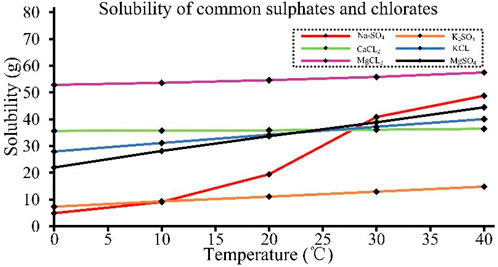
FIGURE 6. Solubility of common sulfates and chlorates along the QGE.

As for sulfates, there is salt expansion by the means of cubical expansions followed by temperature variation. When the contents of SO₄^2- are higher than 1400 mg/L, as the major material of the road, set cement will react with sulfate, and the gypsum (CaSO₄.2H₂O) will be dissolved, and the volume increase by two times. By taking the Na₂SO₄ as an example, the chemical formula can be expressed as

$\mathrm{N}{\mathrm{a}}_2\mathrm{S}{\mathrm{O}}_4\cdot 10{\mathrm{H}}_2\mathrm{O} + \mathrm{C}\mathrm{a}{\left(\mathrm{O}\mathrm{H}\right)}_2 = \mathrm{C}\mathrm{a}\mathrm{S}{\mathrm{O}}_4\cdot 2{\mathrm{H}}_2\mathrm{O} + 2\mathrm{N}\mathrm{a}\mathrm{O}\mathrm{H} + 8{\mathrm{H}}_2\mathrm{O}.(5)$

If the contents of SO₄^2- are low, the solid 4CaOAl₂O₃.12H₂O in the set cement will still react with CaSO₄.2H₂O, and the ettringite (3CaOAl₂O₃.3CaSO₄.31H₂O) crystal will be dissolved out, and it has low solubility. Lots of water crystals (actually, 30–32 H₂O) cause the volume to increase by 2.5 times. Meanwhile, the morphology of the ettringite is an acicular crystal with radial growth. The chemical formula can be expressed as

$3\left(\mathrm{C}\mathrm{a}\mathrm{S}{\mathrm{O}}_4\cdot 2{\mathrm{H}}_2\mathrm{O}\right) + 4\mathrm{C}\mathrm{a}\mathrm{O}\cdot \mathrm{A}{\mathrm{l}}_2{\mathrm{O}}_3·12{\mathrm{H}}_2\mathrm{O} + 14{\mathrm{H}}_2\mathrm{O}= 3\mathrm{C}\mathrm{a}\mathrm{O}\cdot \mathrm{A}{\mathrm{l}}_2{\mathrm{O}}_3\cdot 3\mathrm{C}\mathrm{a}\mathrm{S}{\mathrm{O}}_4\cdot 31{\mathrm{H}}_2\mathrm{O}+\mathrm{C}\mathrm{a}{\left(\mathrm{O}\mathrm{H}\right)}_2(6)$

After these chemical reactions, the strong internal stress to the set cement will be brought, which causes the structural damage and expansion of the uplift.

In the actual environment, Cl⁻ and SO₄^2- always coexist. For the surface concrete, the chemical reactions between SO₄^2- and 4CaOAl₂O₃.12H₂O will be triggered first (chemical formulas (5) and 6). Only after running out of SO₄^2-, Cl⁻ will react with the ettringite (3CaOAl₂O₃.3CaSO₄.31H₂O). For the interior concrete, the chemical reactions between Cl⁻ and OH⁻ will be started first due to the penetrability of Cl⁻ being higher than that of SO₄^2-, the chemical formula can be expressed as

$\mathrm{C}\mathrm{a}{\left(\mathrm{O}\mathrm{H}\right)}_2 + 2\mathrm{C}{\mathrm{l}}^{-} = \mathrm{C}\mathrm{a}\mathrm{C}{\mathrm{l}}_2 + 2\mathrm{O}{\mathrm{H}}^{-}.(7)$

When the contents of Cl⁻ are relatively high, the following chemical reaction will be started too, and it can be expressed as

$3\mathrm{C}\mathrm{a}\mathrm{O}\cdot \mathrm{A}{\mathrm{l}}_2{\mathrm{O}}_3\cdot 6{\mathrm{H}}_2\mathrm{O} + 3\mathrm{C}\mathrm{a}\mathrm{C}{\mathrm{l}}_2 + 25{\mathrm{H}}_2\mathrm{O} = 3\mathrm{C}\mathrm{a}\mathrm{O}\cdot \mathrm{A}{\mathrm{l}}_2{\mathrm{O}}_3\cdot 3\mathrm{C}\mathrm{a}\mathrm{C}{\mathrm{l}}_2\cdot 31{\mathrm{H}}_2\mathrm{O}.(8)$

After these chemical reactions, the ettringite will decrease as well as 4CaOAl₂O₃.12H₂O, and consequently there will be less effect of expansion.

Based on the analyses, we suspect the ratio between Cl⁻ and SO₄^2- (Cl⁻/SO₄^2-) determines the deformation distribution and morphology, and the discussion about deformation results can be conducted as follows.

4.3 The deformation results and discussion

After the DT selection, the time series deformation and velocity can be extracted. Figure 7 shows the line-of-sight (LOS) annual average deformation velocity map from January 2018 to January 2022 based on ascending and descending SAR images. Due to the imaging mechanism of SAR sensors, the observation of InSAR has the highest sensitivity to vertical deformation (Yunjun et al., 2019). In the same area, different deformation appears due to different sensor heading angles, terrain slopes, and aspects (Ferretti et al., 2011; Samiei-Esfahany et al., 2016; Ansari et al., 2018; Yunjun et al., 2019). Even so, two independent SAR datasets show consistent deformation trends in most of the study areas. The ascending and descending maximum positive LOS velocity which indicates uplift has reached 18.4 mm/a and 20.3 mm/a, and the maximum negative LOS velocity which indicates subsidence has reached -42.5 mm/a and -33.3 mm/a, respectively, from January 2018 to January 2022. Along the QGE, the uneven deformation areas distribute piecewise which may be driven by different soil types, or hydrogeological conditions. Hence, we divided the study area of QGE into three segments according to the type of sediment traps (as mentioned in Figure 1). Segment A is a lacustrine facies and chemical deposition area (the chainage is from K585+000 to K603+400), segment B is a lacustrine sedimentary area (the chainage is from K603+400 to K606+250), and segment C is a shore lake facies area (the chainage is from K606+250 to K617+250). To capture the characteristics of the deformation, we depicted the ascending and descending accumulated deformation maps of the study segments along the QGE biannually by using the same color bar, as shown in Figure 8 and Figure 9, respectively. We analyzed the biggest and most influential typical deformation areas of these three segments (i.e., areas D1, D2, and D3) to further reveal the temporal physical deformation evolution of the subgrade and pavement along the QGE.

FIGURE 7

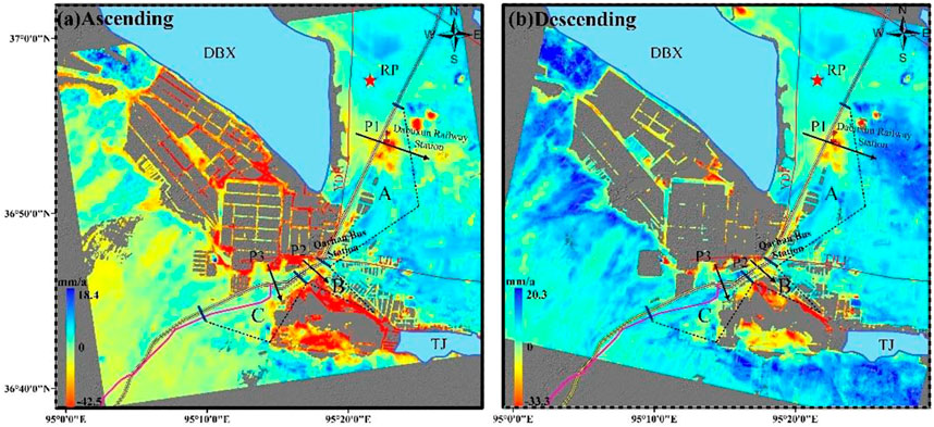
FIGURE 7. LOS Annual average deformation velocity map from 2018 to 2022. The red star indicates the reference point that is selected on a stable artificial structure. The dark blue short-terms represent the chainage break-point of the three different depositional segments (A, B, and C, mentioned in Figure 1). The black arrow lines P1, P2, and P3 denote the typical profile lines of segments A, B, and C. The red lines denote the faults in this area. The red and yellow flags indicate the DRS and QBS, respectively.

FIGURE 8

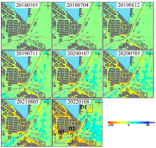
FIGURE 8. Ascending accumulated deformation maps of the study segments along the QGE biannually. The red and yellow flags indicate the DRS and QBS. The red lines denote the faults in this area.

FIGURE 9

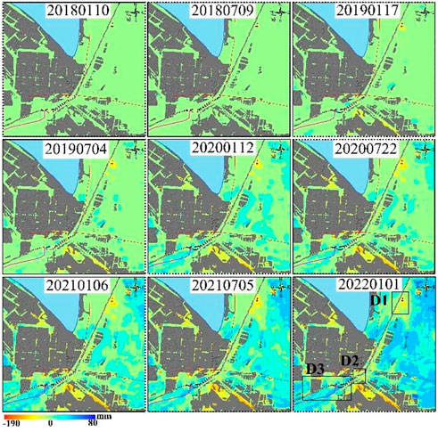
FIGURE 9. Descending accumulated deformation maps of the study segments along the QGE biannually. The red and yellow flags indicate the DRS and QBS. The red lines denote the faults in this area.

According to the engineering geological survey and exploration along the QGE (in the study area), the excessive saline soil is the major part, and the middle saline soil appears in the specific zone (the chainage is from K612+750 to K615+250). Also, the chlorine salt dominates the salt crystal while sulfate salt assists. The ratio between Cl⁻ and SO₄^2- (Cl⁻/SO₄^2-) is from 2.12 to 69.05, and it decreases from north to south along the QGE (Fu, 2011). In addition, the groundwater at the level of 10 m deep will be influenced by the massive extraction of brine and injection of freshwater. In the drilling depth, the organic clay, clay, low liquid limit silt, silty fine sand, and salt crystal comprise the soil layer. As a result, we classify these three segments for piecewise analysis and discussion depending on the different soil layers.

In segment A (lacustrine facies and chemical deposition area, the chainage is from K585+000 to K603+400), we divided it into two subareas (A1 and A2). In subarea A1 (the chainage is from K585+000 to K597+100), the soil layer consists of the salt crystal, organic clay, and clay with interstratified production and different formation thicknesses. The salt crystal distributes widely with transitions from multilayer to a single thin layer, while the thickness gradually thinned out. In the drilling depth, there are three layers of groundwater, the first layer is surface diving, and the second and third layers are the confined brines (the waterhead is from 2 m to 5 m). In subarea A2 (the chainage is from K597+100 to K603+400), the surface is covered with a thickness of 0.05 m–0.1 m salt crust, and the major soil layers are clay with thin salt crystals in the middle, which have moderate dry strength. In the drilling depth, there are two layers of groundwater, the first layer is surface diving (the water level is from 0.4 m to 1.5 m), and the second layer is the confined brines (the waterhead is from 2 m to 5 m). The damage to subgrade and pavement can be caused easily due to the normal engineering properties (Fu, 2011; Shao, 2012). Continuous deformation is crucial for the subgrade and pavement rather than sporadic deformation areas or points. In these two subareas, the continuous settlement is the major deformation along the QGE, especially in area D1 (around the DRS, which belongs to subarea A2). As shown in Figure 10, there may be a karst depression around the DRS. Hence, we extracted the profile line (P1) run through the aforementioned area, the results show that the deformation velocity has reached -16 mm/a approximately. In addition, this deformation funnel has an expanding trend from 2018 to 2022 (as shown in Figure 8 and Figure 9) and may continue in the coming years. At the edge of the funnel, the velocity of the QGE reaches -6.3 mm/a and -3.5 mm/a along the ascending and descending LOS directions, respectively.

FIGURE 10

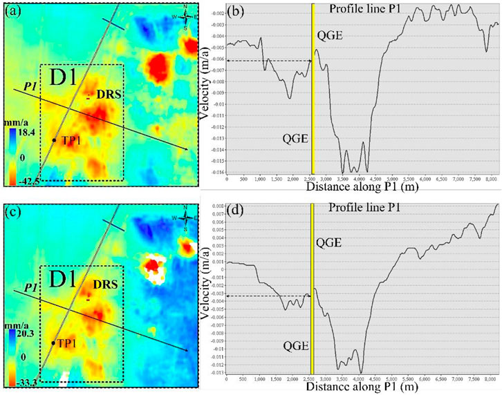
FIGURE 10. Large version LOS annual average deformation velocity map from 2018 to 2022 of area D1 and profile line P1. (A) and (B) indicates the ascending results, (C) and (D) indicate the descending results. The yellow trace represents the location of QGE along the profile line.

It seems like the deformation velocity is acceptable, but the great potential hazards are tough. We obtained the time series deformation of the typical point (TP1 (36.901° N and 95.351° E)) on the QGE. As shown in Figure 11, the fluctuation reflects a typical seasonal characteristic every year. But the cumulative deformation of TP1 in the recent 4 years has reached almost -40 mm, and the fluctuation of settlement is larger uplift relatively, which leads to a long-term deformation existing as settlement without rebounds. From the survey, the hydrophysical condition is severe, such as relatively high levels of groundwater, and soil layers having thin salt crystals in the middle (Fu, 2011). Under the external combined effect of temperature and precipitation, the effect of cyclic freeze–thaw on the water and salt migration, and the reactions between salts and set cement will be intensified. Consequently, the salt swelling and collapsibility occur with a seasonal characteristic. We suspect the key factor of this phenomenon is the high ratio of Cl⁻/SO₄^2-.

FIGURE 11

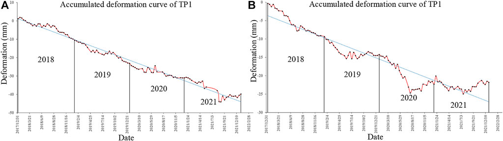
FIGURE 11. Time series deformation of TP1 on the QGE. (A) and (B) indicate the ascending and descending results, respectively.

In segment B (lacustrine sedimentary area, the chainage is from K603+400 to K606+250), the soil layer is silt with moderate dry strength, and the surface diving is the only layer of groundwater (the water level is from 1.4 m to 1.6 m) in the drilling depth (Fu, 2011). As shown in Figure 12, the settlement is still the major deformation phenomenon along the QGE, especially in area D2 (around the QBS). We extracted the profile line (P2) run through the aforementioned area. The velocity of the QGE reaches -8.7 mm/a and -3.4 mm/a along the ascending and descending LOS directions, respectively.

FIGURE 12

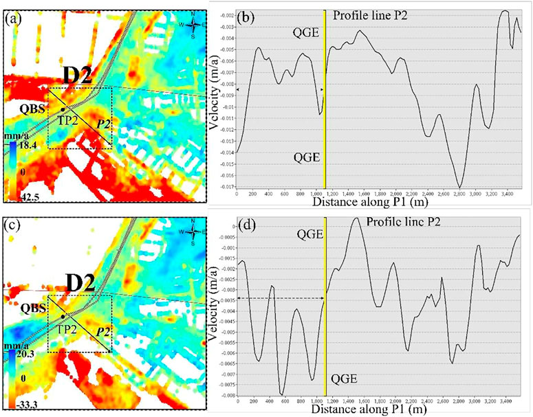
FIGURE 12. Large version LOS annual average deformation velocity map from 2018 to 2022 of area D2 and profile line P2. (A) and (B) indicate the ascending results, (C) and (D) indicate the descending results. The yellow trace represents the location of QGE along the profile line.

As with area D1, the deformation velocity can be ignored easily, whereas the potential hazards still exist. For further revelation, we obtained the time series deformation of the typical point (TP2 (36.79° N and 96.28° E)) on the QGE. As shown in Figure 13, the fluctuation reflects a typical seasonal characteristic every year. But the cumulative deformation in the recent 4 years has reached 25 mm approximately, and the fluctuation of settlement is as large as uplift. It seems like the effects of these two phenomena cancel each other out in a short time, but the long-term deformation still exists as a settlement. In addition, because of the massive extraction of brine and injection of freshwater, the subsidence in the brine pond is tremendous. This powerful effect cannot be neglected due to the QGE being close to the brine pond. From the survey, the groundwater level is relatively deep (Fu, 2011). It is a minor factor while the precipitation and temperature are the major factors. The area D2 is small (as shown in Figure 8 and Figure 9), we speculated that it could be sporadic pavement damage because of the heavy traffic around the bus stations and the local industrial companies. Once cracks appear in the pavement, the precipitation will immerse the subgrade or soil layer. It is accompanied by the reactions between salts and set cement, and the effect of cyclic freeze–thaw on the water and salt migration will be intensified tardily. Considering the curve feature, we suspect that the balanced ratio of Cl⁻/SO₄^2- drives this special phenomenon.

FIGURE 13

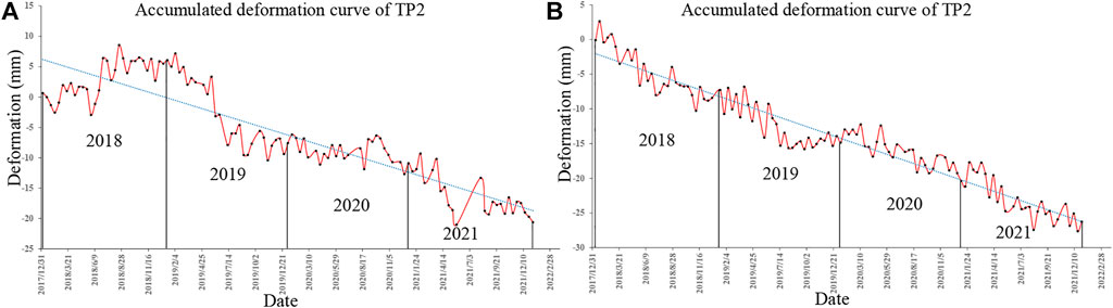
FIGURE 13. Time series deformation of TP2 on the QGE. (A) and (B) indicate the ascending and descending results, respectively.

In segment C (shore lake facies, the chainage is from K606+250 to K617+250), we divided it into two subareas (C1 and C2). In subarea C1 (the chainage is from K606+250 to K615+250), the surface is covered with a thickness of 0.02 m–0.05 m salt crust, and the soil layer is silt fine sand or silty fine sand and is partially filled with silt. The chlorine excessive saline soil is dominant and chlorite excessive saline soil is partial. The groundwater is shallower with pore-type diving. In subarea C2 (the chainage is from K615+250 to K617+250), the upper soil layer is silt with a low liquid limit (belongs to the high compressibility soil) with little salt rust, while the lower soil layer is fine sand with slight liquefaction. In drilling depth, the groundwater is pore-type diving (Fu, 2011).

The uplift is the major deformation phenomenon along the QGE, especially in area D3 (which belongs to subarea C1). As shown in Figure 14, we extracted the profile line (P3) run through the aforementioned area. Different from areas D1 and D2, the opposite deformation trends occur in area D3, the velocity of the QGE reaches 2 mm/a and 7 mm/a along the ascending and descending LOS directions, respectively. The velocity can be easily ignored. However, this area is the most continuous and biggest hazard zone along the QGE. In addition, this deformation funnel has an expanding trend from 2018 to 2022 (as shown in Figure 8 and Figure 9), and maybe it continues to result in a potential threat to the QGE in the coming years.

FIGURE 14

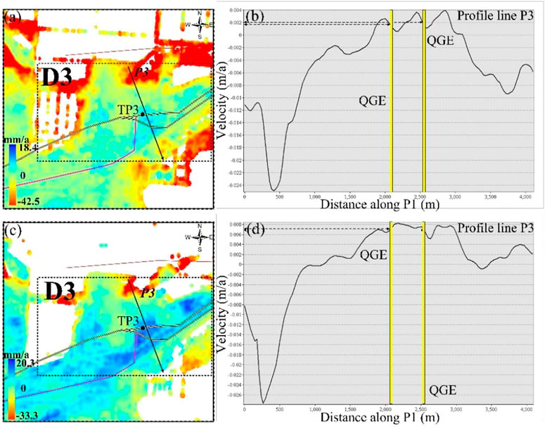
FIGURE 14. Large version LOS annual average deformation velocity map from 2018 to 2022 of area D3 and profile line P3. (A) and (B) indicate the ascending results, (C) and (D) indicate the descending results. The yellow trace represents the location of QGE along the profile line.

For further revelation, we obtained the time series deformation of the typical point (TP3 (36.775° N and 95.239° E)) on the QGE. As shown in Figure 15, the fluctuation reflects a typical seasonal characteristic every year. But the cumulative deformation in the recent 4 years has reached almost 40 mm approximately, and the fluctuation of uplift is larger than settlement relatively, which leads to a long-term uplift without rebounds. From the survey, the groundwater level is relatively deep and results in limited influence. Hence, the precipitation and temperature become the decisive factor. In the rainy season of every year (April to July), the curve fell sharply due to the precipitation in a short time, and rebound quickly once the moisture decreased. The results indicate that the effect of volume expansion is heavier than that of collapse. We also suspect that the small Cl⁻/SO₄^2- drives this phenomenon.

FIGURE 15

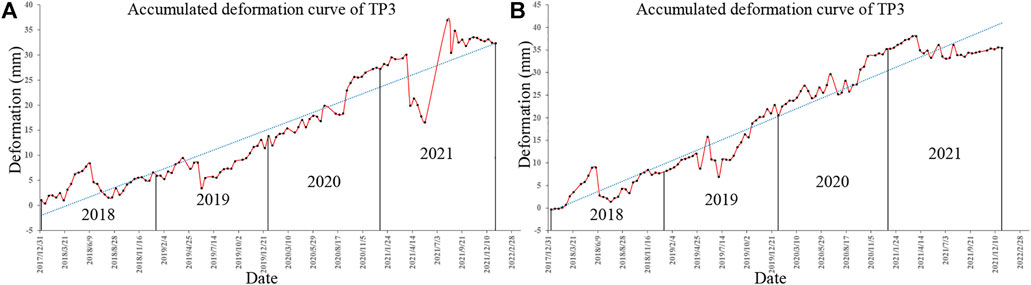
FIGURE 15. Time series deformation of TP3 on the QGE. (A) and (B) indicate the ascending and descending results, respectively.

5 Conclusion

In strong saline soil areas, the engineering properties can be easily affected by water, temperature, human activities (such as massive extraction of brine and injection of freshwater), or other external factors on account of the high environmental sensitivity. Under the circumstance, the subgrade and pavement deformation show a typical seasonal characteristic. To capture the deformation accurately, widely, and continuously, we selected a 32.25 km segment across the QSL of the QGE as the study target by using an advanced MT-InSAR. Considering the previous publications, we sum up the rules for refining the interferogram network directly. Compared with the conventional and previous studies, enough redundant observations are guaranteed, and there is no need to calculate thousands of average interferometric coherence coefficients and perform further analysis. On this basis, the reliable DTs are selected for deformation estimation, and there are almost 0.65 DTs in every pixel (deduct the water area). Both the accuracy, efficiency, and reliability of the monitoring results increased dramatically. Also, we utilized the Poisson curve in the deformation model to describe the temporal physical deformation evolution of the subgrade and pavement over strong saline soil with better reality. Consequently, the time series deformation was extracted based on hundreds of Sentinel-1A images from January 2018 to January 2022. To reveal the deformation characteristics among different sediments, we divided the study targets into three segments for piecewise analysis. Three representative areas along the QGE were discussed based on quantitative analysis of chemical reaction, profile line, and cumulative deformation. The analysis shows that the deformation is mainly affected by the salt expansion, collapsibility, and corrosion directly, which is caused by water (precipitation, meltwater, and injection of freshwater), and temperature. Meanwhile, the ratio between Cl⁻ and SO₄^2- determines the deformation distribution and morphology. Also, the precipitation and temperature affect the seasonal characteristics. Moreover, human activities cannot be neglected, such as the heavy traffic of the local industrial companies. It is an effect of quantitative alteration to qualitative alteration, especially for pavement.

In summary, this study made two contributions to the field. First, we proposed an advanced MT-InSAR based on interferogram seasonal filtering and the Poisson curve to extract time series deformation of the study segments along the QGE. Subsequently, we discussed and analyzed the deformation rules along the study segment of the QGE, and revealed the physical and chemical reasons. The results indicate that the advanced MT-InSAR is adaptive to reflecting the typical seasonal deformation of the expressway subgrade and pavement over strong saline soil. All the related data and information would provide a reliable basis for related transportation management departments in road maintenance.

Data availability statement

The original contributions presented in the study are included in the article/Supplementary Material; further inquiries can be directed to the corresponding author.

Author contributions

Conceptualization, ZW; data curation, ZW; formal analysis, ZW; supervision, SL and YJ; methodology, ZW; resources, XS, YW, and PL; software, HP; visualization, KN; writing–original draft, ZW; writing–review and editing, ZW.

Funding

Research on expressway route selection in western Mountainous areas based on Key technology deformation analysis and system development of InSAR. The funding number is: 2021-YL-08. Application of TS-INSAR technology in urban road collapse prediction. The funding number is: CCX202203.

Acknowledgments

The Sentinel-1A satellite images and the POD data used in this study are provided by the Copernicus Sentinel-1 Mission of ESA. The SRTM DEM data are provided by NASA.

Conflict of interest

All of the authors were employed by Sichuan Highway Planning, Survey, Design and Research Institute Ltd.

The authors declare that the research was conducted in the absence of other any commercial or financial relationships that could be construed as a potential conflict of interest.

Publisher’s note

All claims expressed in this article are solely those of the authors and do not necessarily represent those of their affiliated organizations, or those of the publisher, the editors, and the reviewers. Any product that may be evaluated in this article, or claim that may be made by its manufacturer, is not guaranteed or endorsed by the publisher.

References

Ansari, H., De Zan, F., and Bamler, R. (2018). Efficient phase estimation for interferogram stacks. IEEE Trans. Geosci. Remote Sens. 56 (7), 4109–4125. doi:10.1109/tgrs.2018.2826045

CrossRef Full Text | Google Scholar

Berardino, P., Fornaro, G., Lanari, R., and Sansosti, E. (2002). A new algorithm for surface deformation monitoring based on small baseline differential SAR interferograms. IEEE Trans. Geosci. Remote Sens. 40 (11), 2375–2383. doi:10.1109/tgrs.2002.803792

CrossRef Full Text | Google Scholar

Brouchkov, A. (2003). “Frozen saline soils of the Arctic coast: Their distribution and engineering properties,” in Proceedings of the eighth international conference on permafrost (Zurich, Switzerland), 7, 95–100.

Google Scholar

Castellazzi, G., Colla, C., De Miranda, S., Formica, G., Gabrielli, E., Molari, L., et al. (2013). A coupled multiphase model for hygrothermal analysis of masonry structures and prediction of stress induced by salt crystallization. Constr. Build. Mater. 41, 717–731. doi:10.1016/j.conbuildmat.2012.12.045

CrossRef Full Text | Google Scholar

Cui, S., Pei, X., Jiang, Y., Wang, G., Fan, X., Yang, Q., et al. (2021). Liquefaction within a bedding fault: Understanding the initiation and movement of the Daguangbao landslide triggered by the 2008 Wenchuan Earthquake (Ms= 8.0). Eng. Geol. 295, 106455. doi:10.1016/j.enggeo.2021.106455

CrossRef Full Text | Google Scholar

Dai, K., Li, Z., Xu, Q., Bürgmann, R., Milledge, D., Tomás, R., et al. (2020). Entering the era of earth observation-based landslide warning systems: A novel and exciting framework. IEEE Geosci. Remote Sens. Mag. 8 (1), 136–153. doi:10.1109/mgrs.2019.2954395

CrossRef Full Text | Google Scholar

Ferretti, A., Fumagalli, A., Novali, F., Prati, C., Rocca, F., and Rucci, A. (2011). A new algorithm for processing interferometric data-stacks: SqueeSAR. IEEE Trans. Geosci. Remote Sens. 49 (9), 3460–3470. doi:10.1109/tgrs.2011.2124465

CrossRef Full Text | Google Scholar

Ferretti, A., Prati, C., and Rocca, F. (2000). Nonlinear subsidence rate estimation using permanent scatterers in differential SAR interferometry. IEEE Trans. Geosci. Remote Sens. 38 (5), 2202–2212. doi:10.1109/36.868878

CrossRef Full Text | Google Scholar

Fu, Y. (2011). Study on the technology of dealing with strong saline soil ground of cha-Ge expressway. Xi’an, China: Chang’an University.

Google Scholar

Hu, X., Lu, Z., Oommen, T., Wang, T., and Kim, J. (2017). “Monitoring and modeling tailings impoundment settlement near Great Salt Lake (UTAH) using multi-platform time-series InSAR observations,” in 2017 IEEE international geoscience and Remote sensing symposium (IGARSS) (IEEE), 40–43.

CrossRef Full Text | Google Scholar

Jianjun, Z. H. U., Zhiwei, L. I., and Jun, H. U. (2017). Research progress and methods of InSAR for deformation monitoring. Acta Geod. Cartogr. Sinica 46 (10), 1717.

Google Scholar

Konsta-Gdoutos, M. S. (2006). Monitoring and modeling concrete properties. Netherlands: Springer.

Google Scholar

Li, H., He, Y., Xu, Q., Deng, J., Li, W., and Wei, Y. (2022). Detection and segmentation of loess landslides via satellite images: A two-phase framework. Landslides 19 (3), 673–686. doi:10.1007/s10346-021-01789-0

CrossRef Full Text | Google Scholar

Li, S. S., Li, Z. W., Hu, J., Sun, Q., and Yu, X. Y. (2013). Investigation of the seasonal oscillation of the permafrost over Qinghai-Tibet Plateau with SBAS-InSAR algorithm. Chin. J. Geophys. 56 (5), 1476–1486.

Google Scholar

Li, T. (2014). Deformation monitoring by multi-temporal InSAR with both point and distributed scatterers. Chengdu, China: Southwest Jiaotong University.

Google Scholar

Liao, M., and Wang, T. (2014). Time series insar technology and application. Beijing, China: Science Press, 83–86.

Google Scholar

Liu, G., Ding, X., Chen, Y., Zhi, L. I., and Zheng., D. (2000). New and potential technology for observation of Earth from space: synthetic aperture radar interferometry. Adv. Earth Sci. 15 (6), 734–740.

Google Scholar

Massonnet, D., Rossi, M., Carmona, C., Adragna, F., Peltzer, G., Feigl, K., et al. (1993). The displacement field of the Landers earthquake mapped by radar interferometry. nature 364 (6433), 138–142. doi:10.1038/364138a0

CrossRef Full Text | Google Scholar

Ming-hua, Z. H. A. O., Yu, L. I. U., and Wen-gui, C. A. O. (2005). Study on variable-weight combination forecasting method of S-type curves for soft clay embankment settlement. Rock Soil Mech. 26 (9), 1443–1447.

Google Scholar

Rui, Z., Wei, X., Guoxiang, L. I. U., Xiaowen, W. A. N. G., Wenfei, M. A. O., Yin, F. U., et al. (2021). Interferometric coherence and seasonal deformation characteristics analysis of saline soil based on Sentinel-1A time series imagery. J. Syst. Eng. Electron. 32 (6), 1270–1283. doi:10.23919/jsee.2021.000108

CrossRef Full Text | Google Scholar

Samiei-Esfahany, S., Martins, J. E., Van Leijen, F., and Hanssen, R. F. (2016). Phase estimation for distributed scatterers in InSAR stacks using integer least squares estimation. IEEE Trans. Geosci. Remote Sens. 54 (10), 5671–5687. doi:10.1109/tgrs.2016.2566604

CrossRef Full Text | Google Scholar

Shao, L. (2012). Study on subgrade water and salt migration law and cut off layer setting technology in qarhan Salt Lake area. Xi’an, China: Chang’an University.

Google Scholar

Stipho, A. S. (1985). On the engineering properties of salina soil. Q. J. Eng. Geol. Hydrogeology 18 (2), 129–137. doi:10.1144/gsl.qjeg.1985.018.02.02

CrossRef Full Text | Google Scholar

Wang, D., Liu, J., and Li, X. (2016). Numerical simulation of coupled water and salt transfer in soil and a case study of the expansion of subgrade composed by saline soil. Procedia Eng. 143, 315–322. doi:10.1016/j.proeng.2016.06.040

CrossRef Full Text | Google Scholar

Wei, H. C., Fan, Q. S., An, F. Y., Shan, F. S., Ma, H. Z., Yuan, Q., et al. (2016). Chemical elements in core sediments of the qarhan Salt Lake and palaeoclimate evolution during 94-9 ka. Acta Geosci. Sin. (2), 193–203.

Google Scholar

Wu, Q., and Zhu, Y. (2002). Experimental studies on salt expansion for coarse grain soil under constant temperature. Cold regions Sci. Technol. 34 (2), 59–65. doi:10.1016/s0165-232x(01)00048-9

CrossRef Full Text | Google Scholar

Xiang, W., Zhang, R., Liu, G., Wang, X., Mao, W., Zhang, B., et al. (2022). Extraction and analysis of saline soil deformation in the Qarhan Salt Lake region (in Qinghai, China) by the sentinel SBAS-InSAR technique. Geodesy Geodyn. 13 (2), 127–137. doi:10.1016/j.geog.2020.11.003

CrossRef Full Text | Google Scholar

Xiang, W., Zhang, R., Liu, G., Wang, X., Mao, W., Zhang, B., et al. (2021). Saline-soil deformation extraction based on an improved time-series InSAR approach. ISPRS Int. J. Geoinf. 10 (3), 112. doi:10.3390/ijgi10030112

CrossRef Full Text | Google Scholar

Yang, Z. F., Yi, H. W., Zhu, J. J., Li, Z. W., Su, J. M., and Liu, Q. (2016). Spatio-temporal evolution law analysis of whole mining subsidence basin based on InSAR-derived time-series deformation. Trans. Nonferr. Met. Soc. China 26, 1515–1522.

Google Scholar

Yunjun, Z., Fattahi, H., and Amelung, F. (2019). Small baseline InSAR time series analysis: Unwrapping error correction and noise reduction. Comput. Geosciences 133, 104331. doi:10.1016/j.cageo.2019.104331

CrossRef Full Text | Google Scholar

Zhang, Y., Fang, J., Liu, J., and Xu, A. (2018). Experimental research on physical properties of saline soil subgrade filler in Chaerhan region. Sci. Cold Arid Regions 7 (3), 212–215.

Google Scholar

Zhang, Y., Liu, J., Fang, J., and Xu, A. (2018). Deformation properties of chloride saline soil under action of a low-temperature environment and different loads. Sci. Cold Arid Regions 9 (3), 307–311.

Google Scholar

Zhang, Y., Wu, H. A., and Sun, G. (2012). Deformation model of time series interferometric SAR techniques. Acta Geod. Cartogr. Sinica 41 (6), 864–869.

Google Scholar

Zhu, L., Xing, X., Zhu, Y., Peng, W., Yuan, Z., and Xia, Q. (2021). An advanced time-series InSAR approach based on poisson curve for soft clay highway deformation monitoring. IEEE J. Sel. Top. Appl. Earth Obs. Remote Sens. 14, 7682–7698. doi:10.1109/jstars.2021.3100086

CrossRef Full Text | Google Scholar

Zhu, Z. D., and Zhou, L. H. (2009). Application of Logistic model in settlement prediction during complete process of embankment construction. Chin. J. Geotechnical Eng. 31 (6), 965–969.

Google Scholar