Propagation path tracing of hydraulically created fractures based on microseismic monitoring

To evaluate the effect of hydraulic fracturing in a low-permeability reservoir, a propagation path tracing method for hydraulically created fractures was established based on microseismic monitoring data. First, the numerical simulation of the wave propagation process, grid search, and error-weight coefficient method was combined to locate the microseismic source. Then, the moment tensor inversion method was used to determine the tensile angle and source mechanism of hydraulically created fractures. Next, the tensile angle was used as the weight-index to determine the size of the mixed-source mechanism fracture combined with the shear and tensile source size quantization model. Finally, the spatial topological relationship between fractures was determined by comprehensively considering the spatial location and radius of the fractures, to realize the propagation path tracing of hydraulically created fractures. These tracking results can be used as one of the bases for the evaluation of the hydraulic fracturing effect.

1 Introduction

Hydraulic fracturing is a method to produce cracks in rock strata by using high-pressure liquid to overcome in-situ stress and rock strata strength (Ma et al., 2017; Cui et al., 2021; Zhou et al., 2021), and this method is widely used to improve the permeability and production of low-permeability oil and gas fields. When the reservoir of oil and gas fields breaks under the action of water pressure, the strain energy accumulated in the reservoir will get released, and propagate microseismic waves outwards. Hence, the microseismic monitoring system can be used to collect and analyze the microseismic waves to evaluate the fracturing effect of the reservoir.

In recent years, microseismic monitoring has been widely used in the development of unconventional resources because the productivity is mainly controlled by the fracture network, and the fracture location in the reservoir and the complexity of the fracture network can be speculated based on the analysis of the microseismic monitoring results (Woo et al., 2017). Lin and Zhang. (2016) proposed a method to characterize the fracture zone by the reverse time scale (RTM) of the micro-shear waveform. Through the RTM of the current microseismic waveform, the fracture zone formed in the previous stage can be determined by imaging the strong earthquake zone. Zhu et al. (2017)used the improved signal-filtering method, the time-window energy eigenvalue method of the first arrival selection, and the four channel combination algorithm for determining the source-position to obtain high-precision source-location of microseismic events recorded in a field hydraulic fracturing test in the Huafeng Coal Mine; on these bases, these authors drew the frequency and energy contours of the microseismic events to describe the development and propagation of fractures. Li et al. (2020) conducted hydraulic fracturing and microseismic monitoring simultaneously in shale-gas wells and evaluated the microseismic source location based on guided real-time fracture operation and fracture effect.

The complexity of the fracture network can be further speculated based on the analysis of the microseismic source spatial location (Maxwell et al., 2002; Li et al., 2022; Li et al., 2021a). For example, based on the short-time average/long-time average (STA/LTA) method, interference signal recognition method (ISR), and improved Akaike information criterion (AIC) methods. Li et al. (2021b) characterized the spatial shapes of fractures caused by hydraulic fracturing in coal mines. Aminzadeh et al. (2013) determined the migration direction of the fracture network based on the seismic-source spatial location by using the fuzzy clustering method. Zhang et al. (2019) speculated the fracture propagation path based on the order of occurrence and the spatial distance between the microseismic sources, but they did not consider the crack scale and the topological relationship between cracks, which reduces the reliability of path-prediction results.

The moment-tensor inversion method can be used to infer the source mechanism, and the direction of hydraulic fracturing cracks in reservoirs (Baig and Urbancic, 2010; Li N. et al, 2021; He and Kusiak, 2017). For example, Urbancic et al. (2012) found that the source mechanism of cracks formed by hydraulic fracturing was very complex, and that the source mechanisms can be mainly characterized by tension, compression, or shear. Warpinski et al. found that the crack direction tended to be consistent with the primary cracks, indicating that the activation of primary cracks was one of the main reasons behind the microseismic waves getting induced (Warpinski and Du, 2010). Combining the source-spatial location, the moment-tensor inversion results, and the quantification of the source scale, the discrete fracture network can be established to describe the spatial distribution of reservoir fractures. For example, Ardakani et al. (2018) evaluated the fracturing effect by quantifying the topological relationship of discrete fracture network in different regions. However, since the influence of source mechanism on the fracture scale was not considered, there was a certain error in the quantification of the topological relationship.

In view of the abovementioned problems, this article establishes a crack propagation path tracking method considering the influence of the source mechanism on the crack scale and the topological relationship between cracks and applies this method to an oilfield.

2 The crack propagation path tracing method

The crack propagation path tracing method consists of five steps. Step 1: source location, the numerical simulation of wave-propagation process, grid search, and error-weight coefficient method are combined to locate the microseismic source. Step 2: source-mechanism judgment, the moment-tensor inversion method is used to determine the tensile angle and source mechanism. Step 3: crack-scale quantification, the tensile angle is used as weight-index to determine the size of the mixed-source mechanism fracture combined with shear and tensile source-size quantization model. Step 4: crack topological-relation judgment, where the spatial topological relationship (separation, proximity, and intersection) between fractures is determined by the spatial location and radius of the fractures. Step 5: crack propagation path establishment, where the adjacent or intersecting cracks are connected by line segments to establish the crack propagation tracing path. The flow chart of crack propagation path tracing method is shown in Figure 1, and the detailed principle and data analysis process will be introduced in the following sections.

FIGURE1

FIGURE1. Flow chart of crack propagation path tracing method.

2.1 Source location

Substep 1: Establish and mesh the three-dimensional solid geological model according to engineering geological conditions. Assign physical and mechanical parameters such as wave velocity to mesh units belonging to different strata. In order to balance the accuracy and amount of the calculation, the grid scale near the hydraulic fracturing zone is smaller, and the grid scale far away from the hydraulic fracturing zone is larger. The grid scale range L_M around the hydraulic fracturing zone is set as follows:

$\frac{V_P}{S_f}<L_M<e_{\max },(1)$

where V_P is the propagation velocity of P wave in rock mass, m/s; S_f is the sampling frequency of the microseismic monitoring system, Hz; e_max is the maximum error that meets the positioning requirements, m.

Substep 2: Apply an instantaneous step force (as virtual source) at the nodes of the grid and simulate the propagation process of microseismic wave induced by the instantaneous step force. The time interval at which the instantaneous step force is applied should ensure that the microseismic wave induced by the previous instantaneous step force has propagated to the position of all microseismic sensors. The time interval Δt can be set according to the following:

$\mathrm{\Delta }t=\frac{\sqrt{L^2+W^2+H^2}}{V_P}(2)$

where L, W, and H are the length, width, and height of the numerical model, respectively.

Substep 3: Determine the moment when the instantaneous step force is applied and the moment when the stress wave induced by the instantaneous step force propagates to the position of each microseismic sensor, and then calculate the simulated arrival time difference matrix, ΔT_ij, for microseismic wave propagating from grid node to each microseismic sensor through the following formula:

$\mathrm{\Delta }{T}_{ij}=T_{ij}-T_{i\min }(3)$

where T_ij is the travel-time matrix for the microseismic wave propagating from the grid node, i, to the microseismic sensor j, s; T_imin is the smallest value in the row i of T_ij, s.

Substep 4: Using the microseismic monitoring system installed in the field to collect waveform data, filter the actual microseismic waves, and pick up the actual arrival time, and calculate the actual arrival time difference matrix Δt_kj according to the following formula:

$\mathrm{\Delta }{t}_{kj}=t_{kj}-t_{k\min },(4)$

where t_kj is the arrival-time matrix of kth actual source-induced microseismic wave propagating to microseismic sensor j, s; t_kimin is the smallest value in the row i of t_kj, s.

Substep 5: Match the row vector of the actual arrival time difference matrix, Δt_kj, with the row vector of the simulated arrival time difference matrix, ΔT_ij. If the kth row vector of the actual arrival time difference matrix, Δt_kj, is the same as the ith row vector of the row vector of the simulated arrival time difference matrix, ΔT_ij, the coordinates of the kth microseismic source can then be directly determined as the coordinates of the ith grid node. If not, we select 4 row vectors which are most similar to the actual arrival time difference vector in the simulated arrival time difference matrix, that is, the four row vectors with the minimum sum of absolute deviations, use these deviations as the weight coefficient to locate the microseismic source as follows:

$\begin{array}{l}{c}_k=\frac{S_{k1}{\displaystyle \sum _{p=\mathrm{2,3,4}}{e}_{kp}}}{{\displaystyle \sum _{p=\mathrm{1,2,3,4}}{e}_{kp}}}+\frac{S_{k2}{\displaystyle \sum _{p=\mathrm{1,3,4}}{e}_{kp}}}{{\displaystyle \sum _{p=\mathrm{1,2,3,4}}{e}_{kp}}}+\frac{S_{k3}{\displaystyle \sum _{p=\mathrm{1,2,4}}{e}_{kp}}}{{\displaystyle \sum _{p=\mathrm{1,2,3,4}}{e}_{kp}}}+\frac{S_{k4}{\displaystyle \sum _{p=\mathrm{1,2,3}}{e}_{kp}}}{{\displaystyle \sum _{p=\mathrm{1,2,3,4}}{e}_{kp}}},\\ ={\displaystyle \sum _{p=\mathrm{1,2,3,4}}{S}_{kp}}-\frac{e_{k1}{S}_{k1}+e_{k2}{S}_{k2}+e_{k3}{S}_{k3}+e_{k4}{S}_{k4}}{{\displaystyle \sum _{p=\mathrm{1,2,3,4}}{e}_{kp}}},\end{array}(5)$

where c_k is the coordinate of kth actual microseismic source, m; S_k1,S_k2,S_k3, and S_k4 are the grid nodes corresponding to the four row vectors with the minimum sum of absolute deviations, m; e_kp is the total deviation of the time difference between the kth actual microsource and the grid node p, s, which can be expressed as follows:

$e_{kp}={\displaystyle \sum _{j=1}^n\left|\mathrm{\Delta }{T}_{pj}-\mathrm{\Delta }{t}_{kj}\right|}(6)$

where n is the total number of microseismic sensors.

2.2 Source mechanism judgment

According to the moment-tensor inversion method (Grosse and Ohtsu, 2008), the source moment is expressed in the form of a symmetric second-order tensor, where the firs-motion amplitude of the far-field P-wave induced by a fracture A(x), can be determined by

$A\left(x\right)=\frac{C_s{R}_e\left(t,r\right)e^{-\frac{\pi f}{v_{p}Q}R}}{R}\left(r_1,r_2,r_3\right)\left(\begin{array}{ccc}{m}_{11}& m_{12}& m_{13}\\ m_{12}& m_{22}& m_{23}\\ m_{13}& m_{23}& m_{33}\end{array}\right)\left(\begin{array}{c}{r}_1\\ r_2\\ r_3\end{array}\right)(7)$

where C_s is the magnitude of the sensor response including material constants, R_e(t,r), where R_e is the reflection coefficient, t is the direction of the sensor, r = (r₁, r₂, r₃) is the direction vector from the source to the sensor, R is the distance between the source and the receiving point, v_p is the P wave velocity, Q is the quality factor for P-wave, and f is the frequency which can be replaced either by corner frequency or main frequency.

The source is actually a crack with a certain area. The crack expanded from the initiation point to the final shape in a very short time. If the source mechanism is constant during expansion of the crack, the source mechanism corresponding to the crack initiation point can represent the source mechanism of the whole crack. The simplified green’s function moment tensor inversion method treats the source as a point source formed instantaneously and the source mechanism of the point source determined by the method is the source mechanism corresponding to the initiation point of the crack. Therefore, the point source hypothesis is not inconsistent with the source with a certain area.

When the microseismic wave induced by the same source triggers more than six sensors, the moment tensor of the source can be solved by Eqn. 7, and the motion vector and normal vector of the fracture surface can be further obtained from

$\{\begin{array}{l}\mathbf{n}=\sqrt{\frac{M_1-M_2}{M_1-M_3}}{\mathit{e}}_1+\sqrt{\frac{M_2-M_3}{M_1-M_3}}{\mathit{e}}_3\\ \mathbf{l}=\sqrt{\frac{M_1-M_2}{M_1-M_3}}{\mathit{e}}_1-\sqrt{\frac{M_2-M_3}{M_1-M_3}}{\mathit{e}}_3\end{array}(8)$

where M₁, M₂, M₃ (M₁ > M₂ > M₃) are the three eigenvalues of the moment tensor, and e₁, e₂, e₃ are the eigenvectors corresponding to eigenvalues (M₁, M₂, M₃). (eigenvalue e₂ is missing in the above equation).

The moment tensor is symmetrical, so the vectors l and n are interchangeable. The stress condition can be used to distinguish the motion vector from the normal vector. The crack with a smaller angle with the maximum principal stress is more prone to shear or tensile motion, while the crack with a larger angle with the maximum principal stress is more prone to compression motion. Due to the vertical stress being less than the maximum horizontal principal stress and greater than the minimum horizontal principal stress in the reservoir stratum, the vector with a greater angle with the maximum horizontal principal stress is taken as the normal vector of the crack dominated by shear or tensile component, and the vector with a greater angle with the maximum horizontal principal stress is taken as the normal vector of the compression crack dominated by shear or tensile component.

The source mechanism can be directly judged by the angle between the projection of motion direction, l, on the fracture plane, and the motion direction l, namely, the tensile angle (Kwiatek and Ben-Zion, 2013; Zhang et al., 2020):

$\gamma ={90}^{\circ }-\arccos \left(\mathbf{n}\cdot \mathbf{l}\right)\frac{{180}^{\circ }}{\pi }(9)$

As shown in Figure 2, as the tensile angle, γ, approaches 0°, the proportion of the shear component in the source mechanism gradually increases, which implies that when γ is equal to 0°, the source mechanism is pure shear. As γ approaches −90° or 90°, the proportion of the compression or tension components in the source mechanism increases gradually. When γ is equal to 90°, the source mechanism is pure tension. When the tensile angle γ is equal to −90°, the source mechanism is pure compression, usually implying the compaction of primary cracks.

FIGURE 2

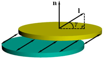
FIGURE 2. Schematic model of source mechanisms.

2.3 Crack scale quantification

According to seismology theory, the crack radius a is inversely proportional to the corner frequency, f_c, of the P- or the S wave (Mendecki, 1996), namely,

$a=K_C\frac{V_C}{f_c},(10)$

where K_C is a constant depending on the source model and V_C is the velocity of the P- or the S wave.

Eqn. 10 can be used for both shear cracks and tension cracks. For the Brune shear model (Brune, 1970), only the S wave is considered, and the coefficient, K_C, is independent of the observation angle, K_C = 0.375. For the Madariaga shear model (Madariaga, 1976), the coefficient, K_C, is a function of the observation angle. After averaging, the coefficient, K_C, for the P wave is 0.21, and the same for the S wave is 0.32. The fracture radius calculated by the Madariaga shear model is about 56% of the Brune shear model. In some mines and underground rock engineering, the fracture radius, calculated by the Madariaga shear model is more in line with the actual observation results (Gibozicz and Kijko, 1994; Trifu et al., 1995). Therefore, this article uses the Madariaga shear model to quantify the shear crack radius. For the Sato tension model (Sato, 1978), the coefficient, K_C, is a function of the observation angle. After averaging, the coefficient, K_C, for the P wave is 0.509, and the same for the S wave is 0.633. Since the motion direction of the rock matrix on both sides of the compression crack is opposite to the direction of the tension crack, the coefficient consistency of the tension model is also used for the compression crack.

As shown in Eqn. 10, the source mechanism is one of the factors that affect crack radius. Therefore, the proportion of shear component in the source mechanism should also be considered as a factor to quantify the radius of tension-shear or compression-shear mixed cracks. The tensile angle is a parameter that can represent the proportion of shear components. In this article, the square of the trigonometric function value of tensile angle is used as the weight coefficient and the radius of shear-tension or shear-compression mixed cracks can be calculated by the weight-coefficient method, that is,

$a_{mix}={\cos }^2\gamma a_s+(1-{\cos }^2\gamma )a_{t/c},(11)$

where a_mix is the radius of the crack with mixed-source mechanism, a_s is the crack radius when the crack is regarded as a shear crack, and a_t/c is the crack radius when the crack is regarded as a tensile crack.

2.4 Crack topological relation judgment

Considering the calculation error in the crack radius, an increase and a decrease in the crack radius by 5% are regarded as the inner and outer diameters of cracks, respectively. Due to the actual error not being measurable, the determination of the value is subjective. However, the crack radius calculation formula (Eqn. 10) has been proved to be close to the actual observation (Gibozicz and Kijko, 1994; Trifu et al., 1995), so it is reasonable to select a relatively small error value. Then, the spatial topological relations between cracks are divided into three types according to whether the cracks intersect or not: separation, adjacency, and intersection. As shown in Figure 3, if the inner diameters of two cracks (disks) intersect, they are defined as intersection; if one crack in the two cracks intersects only with the outer diameter of another crack (regardless of the inner and outer diameters), they are defined as adjacency; if the two cracks are completely separated, they are defined as separation.

FIGURE 3

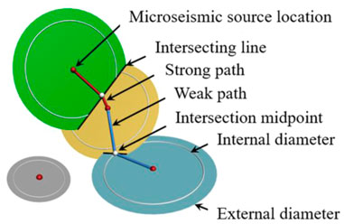
FIGURE 3. Schematic diagram of the fracture propagation path.

2.5 Crack propagation path tracking

Each microseismic source represents a rock fracture at its corresponding position. The increase in the number of fractures, and fracture-expansion coalescence are the fundamental reasons for the macroscopic failure of the rock. Therefore, crack-occurrence time and spatial-topological relationship between the cracks can be used to analyze the spatio-temporal evolution of the hydraulically created fractures.

The intersection-line midpoint of two adjacent or intersecting cracks can be used to connect centers, and then the crack propagation path can be traced by the network of line-segment pairs. The line-segment pairs connecting the adjacent cracks (shown in blue) and the intersecting cracks (shown in red) are called the weak and strong paths, respectively. With the increase in the number of cracks, the topological relationship between the new cracks and the previous cracks is continuously judged, and then the crack propagation path is updated.

In consideration of the error in the calculation of the crack scale, strong and weak paths are used to distinguish the possibility of intersection. Weak paths mean that the possibility of intersection is relatively low, while strong paths mean that the possibility of intersection is high.

3 Engineering application

3.1 Project profile

An oil well is located in Dongying, Shandong Province, China. The oil reservoir is a low-permeability glutenite, and the vertical depth of the oil well is 3,850 m. In order to evaluate the fracturing effect, 16 fully built-in ground microseismic monitoring stations (green columns Table 1 and Figure 4) were installed to monitor the microseismic wave induced by hydraulic fracturing with a sampling frequency of 1,000 Hz.

TABLE 1

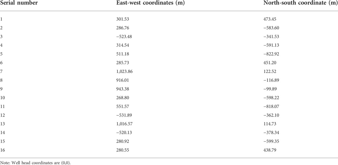
TABLE 1. The coordinates of ground microseismic monitoring stations.

FIGURE 4

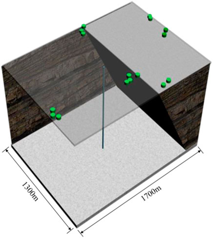
FIGURE 4. Microseismic monitoring stations layout.

During the monitoring period, the well underwent two stages of hydraulic fracturing. In the first stage, the vertical depth-range of the perforation section was 3,605.3 m–3607.7 m, 3,617.7 m–3619.0 m, and 3,622.6 m–3623.8 m, and the total vertical length was about 5 m. In the second stage, the vertical depth-range of the perforation section was 3,581.6 m–3585.2 m, and the vertical total length was about 3.6 m, and the vertical distance between the two stages was about 20 m.

3.2 Sonic velocity in the stratum

The well-logging speed of the oil well is shown in Figure 5. According to the variation characteristics of the wave velocity, the depth was divided into six sections, and the distinguishing depths of each section are: 476.25, 1522.5, 2735, 3005, and 3,160 m. The piece-wise linear-fitting method was used to simplify the variation of the wave velocity with depth and the fitting results were used as the wave velocity input of microseismic source location.

FIGURE 5

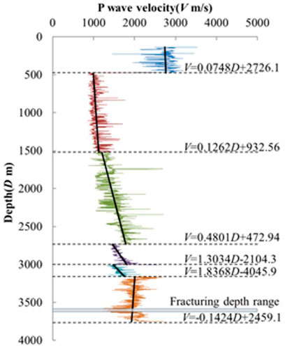
FIGURE 5. Logging velocity and wave velocity fitting.

3.3 Numerical simulation of the microseismic wave propagation process

A 1600 m × 1,350 m × 3,750 m (length × width × height) numerical model of the oil well was established, and the scale of the grid element in the fracturing area was 10 m (Figure 5). The initial pressure set by the oil well was set to 0 MPa, and the displacement constraints were imposed on the side and the bottom of the numerical model. Since only the arrival time of the microseismic wave was needed, the boundaries of the numerical model were set as a complete transmission boundary in order to reduce the calculation amount and improve the calculation efficiency. The P-wave velocity corresponding to the grid unit was determined according to the piece-wise fitting formula (Figure 6).

FIGURE 6

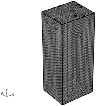
FIGURE 6. Calculation model.

In the fractured zone and its adjacent area (depth range of ∼3,550 m–3,650 m), instantaneous step force was applied on the element grid nodes in turn. The propagation process of the microseismic wave induced by the instantaneous step force was simulated using the acoustic module of COMSOL Multiphysics multi-physical field analysis software. The control equation used in the simulation is as follows:

$\frac{1}{\rho c^2}\frac{{\partial }^2{p}_t}{\partial t^2}+\nabla \cdot \left(-\frac{1}{\rho }\left(\nabla p_t-q_d\right)\right)=Q_m,(12)$

where p_t is the total acoustic pressure, ρ is the fluid density, c is the speed of the microseismic wave, q_d is the dipole domain source, and Q_m is the monopole domain source.

Figure 7 shows the propagation process of the microseismic wave induced by the instantaneous step force at (0, 0, 3,617) in the numerical model. Figure 8 shows the simulated microseismic wave propagation from the instantaneous step force to each sensor. From the waveform diagram, the simulated arrival-time matrix of the microseismic wave to 16 sensors is obtained (Table 2), and the simulated time-difference matrix is calculated according to Eqn. 4 (Table 3).

FIGURE 7

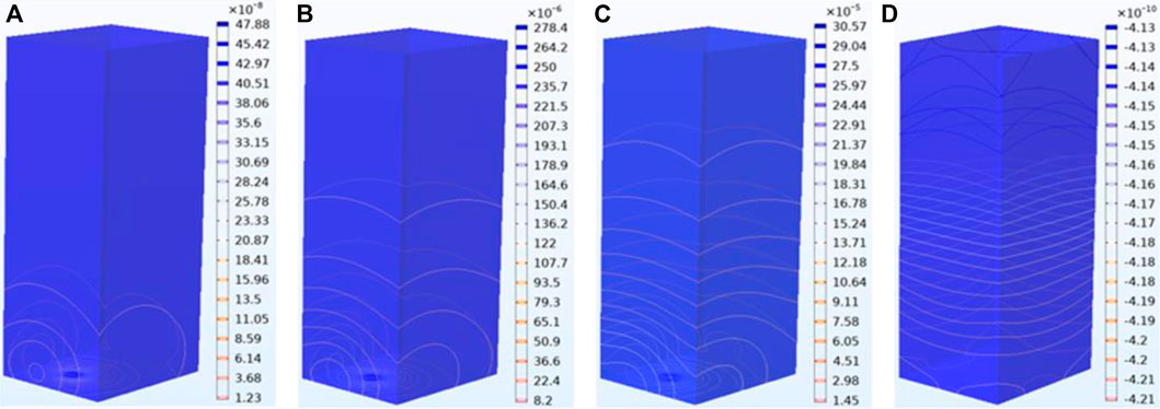
FIGURE 7. Total sound pressure isoline (Pa). (A), 1E-4s; (B), 7E-4s; (C), 9E-4s; (D), 6.45E-3s.

FIGURE 8

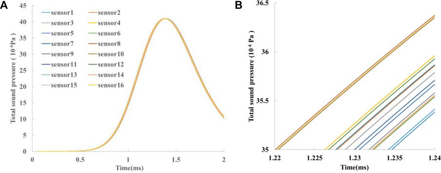
FIGURE 8. Simulation waveform and arrival time picking. (A), Simulation waveform; (B), Arrival time picking.

TABLE 2

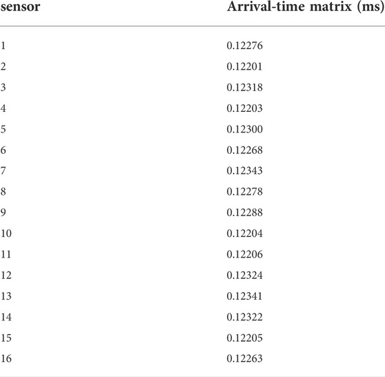
TABLE 2. Arrival-time matrix.

TABLE 3

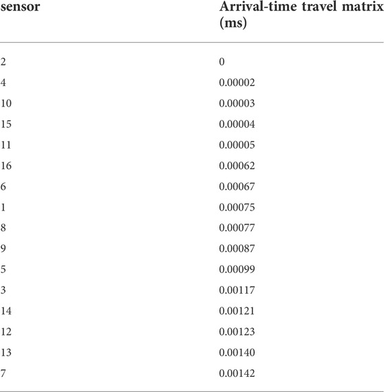
TABLE 3. Time-difference matrix.

3.4 Spatial distribution of hydraulic fracturing cracks

The waveform collected by the station in the process of hydraulic fracturing, and the method described in Section 1 were used for data processing as the basic data for analyzing the evolution of the fracturing crack propagation path in this article.

A total of 127 and 137 microseismic sources were induced in the first- and second-stage fracturing, respectively. Based on the microseismic monitoring data, the discrete fracture network representing the fracturing crack was generated, as shown in Figure 9. The center point of the disk is the location of the microseismic source, and the radius of the disk represents the radius of the crack, and different colors correspond to different tensile angles.

FIGURE 9

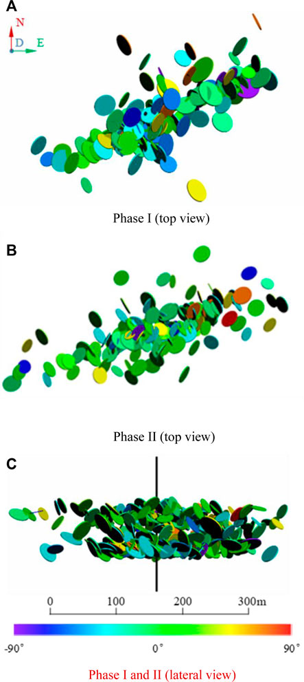
FIGURE 9. Microseismicity-derived discrete fracture network for different fracturing stages. (A), Phase I(top view); (B), Phase II(top view); (C), Phase I and II (lateral view).

The cracks induced by hydraulic fracturing in the two stages are mainly extended in the northeast and southwest directions, and the propagation direction of the second stage is closer to the east-west direction than that of the first stage. The maximum propagation ranges of the first- and the second-stage fracturing are 346.8 and 395.0 m, respectively (Figures 9A,B).

The tensile angle ranges from −86.3°∼89.2°, indicating that the source mechanism of the cracks is complex, but the tensile angle of more than 82% cracks is between −45° and 45°, indicating that most cracks are still dominated by shear although they are accompanied by a certain degree of compression or tension components.

The crack diameter ranges from 15.1 to 42.4 m. Although the perforating sections of the two fracturing stages are 20 m apart, it can be observed from the side-view of the spatial distribution of the discrete fracture network (Figure 9C) that the cracks induced by the two fracturing stages got interconnected.

3.5 Crack propagation path

The spatial distribution of the crack propagation path in the two fracturing stages is shown in Figure 10. As shown in Figures 10A,B. 10a, most cracks are connected with each other through strong and weak paths to form a main crack propagation path with complex morphology, which is also the main seepage channel of the fracturing fluid.

FIGURE 10

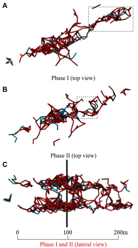
FIGURE 10. Fracture propagation path at different fracturing stages. (A), Phase I(top view); (B), Phase II(top view); (C), Phase I and II (lateral view).

At the same time, in the area far away from the wellbore, there are also some minor crack propagation paths whose length and complexity are far lower than those of the main crack propagation path, and they are not connected with the main crack propagation paths. The formation of these minor crack propagation paths can be attributed to the stress disturbance of the hydraulic fracturing process on the initial stress field of the reservoir where the fracturing fluid did not reach.

Generally, the complexity of the crack propagation path increases first and then decreases with increasing distance between the wellbore and the crack. However, due to the influence of the spatial distribution of the primary crack, the complexity would include severe fluctuations in some local area; for example, the complexity of the crack propagation path in the northeast direction of the wellbore increases again after the decrease (the area shown by the dotted line in Figures 10A,B).

It can be seen in Figure 10C that the crack propagation paths formed by the first and second stages of fracturing have multiple interconnected strong paths and weak paths, indicating that the cracks formed by the two fracturing stages got interconnected. The depth of the crack propagation path in the first stage fracturing ranges from 3,589 m to 3,644 m (height difference of 55 m), and the depth of the crack propagation path in the second stage fracturing ranges from 3,566 m to 3,593 m (height difference of 27 m). The depth-range of the crack propagation path in the second stage is smaller than that of the same in the first stage. The main reason for this phenomenon is that the perforating range of the second stage is smaller than that of the first stage, and the mutual penetration of the cracks in the two stages will also inhibit the upward propagation of cracks in the second stage.

4 Conclusion

Based on the microseismic monitoring data, this study established a method for tracing the propagation path of hydraulic fracturing cracks, and used this method to quantify and analyze the spatial distribution, source mechanism, and propagation path of fracturing cracks in an oil well. The main conclusions are as follows:

1 The cracks formed by hydraulic fracturing mainly extend to the northeast and southwest directions, and the source mechanism of the cracks is relatively complex. Most of the cracks are dominated by shear, and accompanied by compression or tension components to a certain extent.

2 Most cracks induced by hydraulic fracturing connect with each other, and form a complex main crack propagation path, which provides the main seepage channel for the fracturing fluid. At the same time, some minor crack propagation paths that are not connected with the main crack propagation path can also be induced by stress disturbance.

3 There are multiple interconnected strong and weak paths between the first and second fracturing stages, indicating that the cracks formed in the two stages of fracturing have penetrated each other, and the penetration of such cracks inhibits the upward propagation of the cracks in the second stage of fracturing, resulting in the depth range of the crack propagation path in the second stage that is less than that in the first stage.

Data availability statement

The raw data supporting the conclusions of this article will be made available by the authors, without undue reservation.

Author contributions

LH-L contributed to the conception and design of the whole study. HH-T and ZP-H analyzed the research content, and HH-T and ZP-H wrote the first draft of the manuscript. HJ-X conducted relevant numerical simulation, and LL-C, ZL-Y, and ZZ-L conducted engineering application research. All authors participated in the revision of the manuscript and read and approved the submitted version.

Funding

The work presented in this article was financially supported by the National Natural Science Foundation of China (52174070 and 51879041) and Fundamental Research Funds for the Central Universities of China (N2201015 and N2101040).

Conflict of interest

Authors ZL‐Y and ZZ‐L were employed by the company Shengli Oilfield Company, SINOPEC.

The remaining authors declare that the research was conducted in the absence of any commercial or financial relationships that could be construed as a potential conflict of interest.

Publisher’s note

All claims expressed in this article are solely those of the authors and do not necessarily represent those of their affiliated organizations, or those of the publisher, the editors, and the reviewers. Any product that may be evaluated in this article, or claim that may be made by its manufacturer, is not guaranteed or endorsed by the publisher.

References

Aminzadeh, F., Tafti, T. A., and Maity, D. (2013). An integrated methodology for sub-surface fracture characterization using microseismic data: a case study at the NW geysers. Comput. Geosciences 54, 39–49. doi:10.1016/j.cageo.2012.10.015

CrossRef Full Text | Google Scholar

Ardakani, E. P., Baig, A. M., Urbancic, T., and Bosman, K. (2018). Microseismicity-derived fracture network characterization of unconventional reservoirs by topology. Interpretation 6 (2), SE49–SE61. doi:10.1190/INT-2017-0172.1

CrossRef Full Text | Google Scholar

Baig, A., and Urbancic, T. (2010). Microseismic moment tensors: A path to understanding frac growth. Lead. Edge 29 (3), 320–324. doi:10.1190/1.3353729

CrossRef Full Text | Google Scholar

Brune, J. N. (1970). Tectonic stress and the spectra of seismic shear waves from earthquakes. J. Geophys. Res. 75 (26), 4997–5009. doi:10.1029/JB075i026p04997

CrossRef Full Text | Google Scholar

Cui, S., Pei, X., Jiang, Y., Wang, G., Fan, X., Yang, Q., et al. (2021). Liquefaction within a bedding fault: Understanding the initiation and movement of the Daguangbao landslide triggered by the 2008 Wenchuan Earthquake (Ms= 8.0). Eng. Geol. 295, 106455. doi:10.1016/j.enggeo.2021.106455

CrossRef Full Text | Google Scholar

Gibowicz, S. J., and Kijko, A. (1994). An introduction to mining seismology. Int. Geophys. Ser. 55, i–x. doi:10.1109/TSTE.2017.2715061

CrossRef Full Text | Google Scholar

He, Y., and Kusiak, A. (2017). Performance assessment of wind turbines: data-derived quantitative metrics. IEEE Trans. Sustain. Energy 9 (1), 65–73. doi:10.1109/tste.2017.2715061

CrossRef Full Text | Google Scholar

Kwiatek, G., and Ben‐Zion, Y. (2013). Assessment of P and S wave energy radiated from very small shear‐tensile seismic events in a deep South African mine. J. Geophys. Res. Solid Earth 118 (7), 3630–3641. doi:10.1002/jgrb.50274

CrossRef Full Text | Google Scholar

Li, H., Deng, J., Feng, P., Pu, C., Arachchige, D. D., Cheng, Q., et al. (2021a). Short-term nacelle orientation forecasting using bilinear transformation and ICEEMDAN framework. Front. Energy Res. 697. doi:10.3389/fenrg.2021.780928

CrossRef Full Text | Google Scholar

Li, H., Deng, J., Yuan, S., Feng, P., and Arachchige, D. D. (2021b). Monitoring and identifying wind turbine generator bearing faults using deep belief network and EWMA control charts. Front. Energy Res. 770. doi:10.3389/fenrg.2021.799039

CrossRef Full Text | Google Scholar

Li, H., He, Y., Xu, Q., Deng, J., Li, W., Wei, Y., et al. (2022). Detection and segmentation of loess landslides via satellite images: a two-phase framework. Landslides 19, 673–686. doi:10.1007/s10346-021-01789-0

CrossRef Full Text | Google Scholar

Li, J., Yu, B. S., Tian, Y. K., Kang, H. X., Wang, Y. F., Zhou, H., et al. (2020). Effect analysis of borehole microseismic monitoring technology on shale gas fracturing in Western Hubei. Appl. Geophys. 17 (5), 764–775. doi:10.1007/s11770-020-0868-9

CrossRef Full Text | Google Scholar

Li, N., Fang, L., Sun, W., Zhang, X., and Chen, D. (2021c). Evaluation of borehole hydraulic fracturing in coal seam using the microseismic monitoring method. Rock Mech. Rock Eng. 54 (2), 607–625. doi:10.1007/s00603-020-02297-8

CrossRef Full Text | Google Scholar

Lin, Y., and Zhang, H. (2016). Imaging hydraulic fractures by microseismic migration for downhole monitoring system. Phys. Earth Planet. Interiors 261, 88–97. doi:10.1016/j.pepi.2016.06.010

CrossRef Full Text | Google Scholar

Ma, X., Zou, Y., Li, N., Chen, M., Zhang, Y., Liu, Z., et al. (2017). Experimental study on the mechanism of hydraulic fracture growth in a glutenite reservoir. J. Struct. Geol. 97, 37–47. doi:10.1016/j.jsg.2017.02.012

CrossRef Full Text | Google Scholar

Madariaga, R. (1976). Dynamics of an expanding circular fault. Bull. Seismol. Soc. Am. 66 (3), 639–666. doi:10.1785/BSSA0660030639

CrossRef Full Text | Google Scholar

Maxwell, S. C., Urbancic, T. I., Steinsberger, N., and Zinno, R. (2002). “Microseismic imaging of hydraulic fracture complexity in the Barnett shale,” in SPE annual technical conference and exhibition, San Antonio, Texas, September 29–October 2, 2002. OnePetro. doi:10.2523/77440-ms

CrossRef Full Text | Google Scholar

A. J. Mendecki (1996). Seismic monitoring in mines. (Berlin, Germany: Springer Science & Business Media).

Google Scholar

Sato, T. (1978). A note on body wave radiation from wxpanding tension crack. Sci. Rep. Tohoku Univ. Geophys. 25 (1), 1–10.

Google Scholar

Trifu, C. I., Urbancic, T. I., and Young, R. P. (1995). Source parameters of mining-induced seismic events: An evaluation of homogeneous and inhomogeneous faulting models for assessing damage potential. pure Appl. Geophys. 145 (1), 3–27. doi:10.1007/BF00879480

CrossRef Full Text | Google Scholar

Urbancic, T., Baig, A., and Goldstein, S. (2012). “Assessing stimulation of complex natural fractures as characterized using microseismicity: an argument the inclusion of sub-horizontal fractures in reservoir models,” in SPE Hydraulic Fracturing Technology Conference, The Woodlands, Texas, USA, February 6–8, 2012. OnePetro. doi:10.2118/152616-ms

CrossRef Full Text | Google Scholar

Warpinski, N. R., and Du, J. (2010). “Source-mechanism studies on microseismicity induced by hydraulic fracturing,” in SPE Annual Technical Conference and Exhibition, Florence, Italy, September 19–22, 2010. OnePetro. doi:10.2118/135254-MS

CrossRef Full Text | Google Scholar

Woo, J. U., Kim, J., Rhie, J., and Kang, T. S. (2017). Characteristics in hypocenters of microseismic events due to hydraulic fracturing and natural faults: a case study in the horn river basin, Canada. Geosci. J. 21 (5), 683–694. doi:10.1007/s12303-017-0021-9

CrossRef Full Text | Google Scholar

Zhang, P. H., Zhang, Z. L., Li, M., and Zhang, L. Y. (2019). Extension process and fracture mechanism of hydraulic fractures in low permeability reservoir. J. Northeast. Univ. Nat. Sci. 40 (5), 745. doi:10.12068/j.issn.1005-3026.2019.05.026

CrossRef Full Text | Google Scholar

Zhang, P., Yu, Q., Li, L., Xu, T., Yang, T., Zhu, W., et al. (2020). The radiation energy of AE sources with different tensile angles and implication for the rock failure process. Pure Appl. Geophys. 177 (7), 3407–3419. doi:10.1007/s00024-020-02430-2

CrossRef Full Text | Google Scholar

Zhou, J., Wei, J., Yang, T., Zhang, P., Liu, F., Chen, J., et al. (2021). Seepage channel development in the crown pillar: Insights from induced microseismicity. Int. J. Rock Mech. Min. Sci. 145, 104851. doi:10.1016/j.ijrmms.2021.104851

CrossRef Full Text | Google Scholar

Zhu, Q., Feng, Y., Cai, M., Liu, J., and Wang, H. (2017). Interpretation of the extent of hydraulic fracturing for rockburst prevention using microseismic monitoring data. J. Nat. Gas Sci. Eng. 38, 107–119. doi:10.1016/j.jngse.2016.12.034

CrossRef Full Text | Google Scholar