Spatially correlated Vs30 estimation in the Beijing area

Beijing is an international metropolis, that is also an earthquake-prone city. The aims of this study are detailed quantifying and qualifying soil layer properties for an accurate seismic safety evaluation in the Beijing area. The time average shear-wave velocity in the first 30 m of subsoil, V_s30, is an important site parameter used in site response analysis, site classification, and seismic loss estimation. Mapping of V_s30 over a city-scaled region is commonly done through proxy-based methods by correlating V_s30 with geological or topographic information. In this paper, a geostatistical-based random field model is presented and applied to mapping V_s30 over extended areas. This random field model is then coupled with Monte Carlo simulations to obtain an averaged V_s30 map and its associated uncertainties. Unlike the traditional deterministic prediction model, this framework accounts for spatial variations of V_s30 values and uncertainties, which makes the prediction more reliable. A total of 388 shear wave velocity measurements in the Beijing area are used to calculate V_s30 values, from which the statistical and spatial properties for the random field realizations are inferred. New spatially correlated probabilistic V_s30 maps for the Beijing area are then represented, and the effect of the maximum number of previously generated elements to correlate to in estimating V_s30 maps is tested.

1 Introduction

The time-averaged shear-wave velocity in the upper 30 m (V_S30) is an important site parameter used in estimating site response, classifying sites, and loss estimation (Boore, 2004; Xie et al., 2016). In the earthquake codes, V_s30 is used with CPT, SPT value and/or the depth of soil profiles to represent the soil properties. Furthermore, some recent studies, show that coupling between V_s30 and other site-condition proxies such as resonance frequency and topographical slope may give efficient results in prediction specified with a reduction of ground-motion variability (Derras et al., 2017; Derras et al., 2020). A reasonable and accurate database of V_s30 is the basis for successfully carrying out seismic effect analysis and research of complex sites and implementing reasonable site classification. However, for large-scale urban areas, the boreholes with shear wave velocity data and meeting the requirements are extremely limited (Seed and Idriss, 1981; Raptakis et al., 1995; Wride et al., 2000; Hasancebi and Ulusay, 2007), which mainly manifested as follows: 1) Boreholes have geotechnical description data but no shear wave velocity data; 2) Because of the different uses of boreholes, the depth of boreholes are different. For example, the depth of boreholes in engineering geotechnical investigation is shallow, even less than 30 m; 3) The boreholes for seismic safety evaluation of major engineering and site control engineering have deep depth and complete wave velocity data, but the number of boreholes is limited and the spatial distribution is uneven. Therefore, in order to meet the needs of urban regional-scale earthquake effect analysis, as well as the requirement of implementing reasonable site classification, it is necessary to accurately describe the complex site conditions with a spatially correlated V_s30 map in urban areas which combines shear wave velocity measurements and a scientific, reasonable and efficient prediction model.

At present, deterministic methods are mostly used in site shear wave velocity predictions. Commonly used deterministic methods can be roughly divided into two categories: 1) Interpolation prediction of parameter distribution between boreholes based on linear interpolation method (Badal et al., 2004), focusing on prediction between two points, but lacking extension ability; 2) According to the regression analysis method in traditional statistical methods, the regression equation between shear wave velocity and topography, geomorphology, depth, CPT-N, and other parameters is established (Wald and Allen, 2007; Chiou and Youngs, 2008; Ancheta et al., 2013; Stewart et al., 2014; Wills et al., 2015; Xie et al., 2016; Ahdi et al., 2017; Parker et al., 2017; Chen et al., 2018; Rahman et al., 2018; Heath et al., 2020). The above deterministic method determines the spatial distribution pattern and correlation by analyzing the frequency distribution or mean value and variance relationship of sample attribute values and their corresponding rules, but does not consider the difference in spatial orientation.

Moreover, the most fatal disadvantage of the deterministic method is that it can’t take into account the uncertainty of parameters. It has been well-recognized that the soil profile and the associated parameters are usually not known with certainty (Liu et al., 2017a,b; Liu et al., 2021; Zhang et al., 2021; Stewart and Afshari, 2021; Ching et al., 2018; Phoon et al., 2022). These uncertainties will eventually be expressed and propagated in further applications such as the uncertainty of site response and the degree of earthquake disasters (Liu et al., 2021). Therefore, other than the accuracy prediction of V_s30 values for a certain region, the uncertainty distribution of V_s30 needs to be evaluated. One thing needs to be noticed, there are many sources of uncertainty, such as insufficient in-situ geotechnical survey data, the influence of sample disturbance and scaling in laboratory tests, and the natural heterogeneity of soil profiles (Ching and Schweckendiek, 2021; Phoon et al., 2022). It is hard to tell them apart. In this paper, the uncertainties from different sources are integrated, and defined as the “uncertainty of V_s30”, regardless of their sources.

To remedy the above defects, the application of geostatistical methods in soil properties (V_s30, CPT, SPT, et al.) and site condition mapping has been greatly promoted, which takes into account the spatial variability of soil properties and the obvious interdependence among points. Several works have been done along this line:

Thompson et al. (2007) use the geostatistical method for modeling the horizontal variability of near-surface shear wave velocity of soil in the San Francisco Bay Area. Wald et al. (2011) and Yong et al. (2013) applied the kriging-with-a-trend method to mapping V_s30 considering the topographic slope. Liu et al. (2017a, b) presented a multiscale random field model and applied it to mapping V_s30 over the Suzhou area, in which areas of high interest can be able to adaptively refined while maintaining a consistent description of spatial dependence. Chen et al. (2018) built a 3D shear wave velocity model for the Suzhou area by using the Kriging method in the horizontal direction. By using the Kriging method, Foster et al. (2019) developed a geology-based and terrain-based models V_S30 map for New Zealand and compared it with a flexible multivariate normal approach. Li et al. (2021) developed a Texas-specific V_S30 map by using the geostatistical kriging method which integrated with a region-specific geologic proxy and field measurements of V_S30. All these works show that by using geostatistical methods, the spatial variation of shear wave velocity can be well considered during estimation.

In this paper, a random field-based approach is presented and adopted to simulate and predict the V_s30 in the study area, more importantly, the uncertainty distribution of V_s30 is evaluated. In the meantime, the effect of the maximum number of previously generated elements to correlate to is also been tested. The presented approach accounts for the spatial variability of V_s30 and incorporates the database of geotechnical measurements. The order of presentation of this paper goes as follows: Section 2 presents the key components of the developed geostatistical tools for mapping V_s30; Engineering geology and field data for the Beijing area are summarized in Section 3; In Section 4, the statistical and spatial characterizations of the known V_s30 data are discussed in detail; New V_s30 maps are represented in Section 5 and the effect of N value in estimating V_s30 maps will be discussed in Section 6.

2 Geo-statistical approach to characterize the spatial variability of V_s30: Random field model

The key component of this section is to present the shear wave velocity estimation model by using the random field method in geostatistical theory. Geostatistical theory shows that the geotechnical or geological characteristics of the regional areas usually show spatial variability and spatial correlation, which means the soil parameters measured at each observation point are correlated with those at adjacent locations, and with the increase of distance, the correlation between the parameters decreases gradually. According to that, this method can be used to simulate various parameters with time-space variation attributes in nature, such as soil characteristics in a certain space range, or ground motion changes at different times and locations. Therefore, it is proposed to use this theory to establish a prediction model of V_s30. With the spatial distribution characteristics of V_s30, the accuracy of V_s30 estimation at unsampled points can be improved. Moreover, other than improving the accuracy of the estimation, one of the strengths of this random field method is the ability to estimate the associated uncertainties with the maps when coupled with Monte Carlo simulation.

Semi-variogram is known as a form of covariance and can be related to other commonly used measures to quantify the spatial correlation (Baise et al., 2006; DeGroot and Baecher, 1993; Goovaerts, 1997). Usually, the filed measured data will be used to fit the best curve of the semi-variogram and expressed as s linear combination of basic models such as the exponential model, spherical model, and Gaussian model. The geo-statistics community is preferred using the semi-variograms to describe the spatial structure since it only requires the increment of the random variable at two locations with distance h to be second-order stationery, which is a weaker requirement. The Hence, in this study, the spatial structure is characterized by the semi-variogram model as follows:

$\gamma \left(h\right)=\frac{1}{2}\mathrm{V}\mathrm{a}\mathrm{r}\left[Z\left(u\right)-Z\left(u+h\right)\right](1)$

In which, $Z\left(u\right)$ is the random variable at location u, and h is the distance between any two locations.

Under the condition of second-order stationarity, the spatial correlation ${\rho }_{\left(h\right)}$ can be defined as related to the semi-variogram by:

${\rho }_{\left(h\right)}=1-\frac{\gamma \left(h\right)}{\mathrm{c}\mathrm{o}\mathrm{v}\left(0\right)}(2)$

where COV(0) is the covariance at h = 0.

With the correlation between the two elements, the covariance matrix Σ consists of the covariance (COV) between any two points/elements (Z_i and Z_j) within the random field t can be calculated as:

$COV\left[Z_i,Z_j\right]={\rho }_{Z_i,Z_j}{\sigma }_{Z_i}{\sigma }_{Z_j}(3)$

where ${\rho }_{Z_i,Z_j}$ is the correlation between the two elements, ${\sigma }_{Z_i}$ and ${\sigma }_{Z_j}$ are the corresponding standard deviations respectively.

Once the covariance between any two elements in the random field is determined, a conditional sequential simulation procedure is taken for the simulation. In this work, it is assumed that the V_s30 obeys lognormal distributions, which can be converted into normal distributions using statistical transformations. Based on the conditional random field theory, the random variable $Z_n$ can be characterized by a joint normal distribution as

$\left[\begin{array}{c}{Z}_n\\ {\mathit{Z}}_p\end{array}\right]\sim N\left(\mathit{\mu },\mathbf{\Sigma }\right)=N\left(\left[\begin{array}{c}{\mu }_n\\ {\mathit{\mu }}_p\end{array}\right],\left[\begin{array}{cc}{\Sigma }_{nn}& {\mathbf{\Sigma }}_{np}\\ {\mathbf{\Sigma }}_{pn}& {\mathbf{\Sigma }}_{pp}\end{array}\right]\right)(4)$

The process simulates each value individually, conditional upon all known data and previously generated values. Using such a process, the conditional distribution of the next value to be simulated in the random field, denoted as Z_n, is given by a univariate normal distribution with the updated mean and the variance as:

$\left(Z_n|Z_p\right)\sim N\left({\Sigma }_{np}\bullet {\Sigma }_{np}^{-1}\bullet Z_p,{\sigma }_n^2-{\Sigma }_{np}\bullet {\Sigma }_{np}^{-1}\bullet {\Sigma }_{pn}\right)(5)$

where Z_p is a vector of all known or previously simulated points; the subscription “p” means “previous” simulated points and “n” refers to the “next” point to be simulated. Once Z_n is generated, it is inserted into the “previous” vector, upon which the “next” unknown value at another unsampled location will be generated. Such a process is repeated until all the values in the field are simulated, and then, a map of V_s30 is generated for the region of interest. The flowchart of the random field implementation is shown in Figure 1.

FIGURE 1

FIGURE 1. Flowchart of the random field model implementation.

3 The Beijing site: Engineering geology and field data

Beijing is an international metropolis and is also one of the capitals of three countries in the world that have suffered earthquakes of magnitude eight or above in history (Peng et al., 2011; Yuan et al., 2019; Peng et al., 2020). Beijing is located at the intersection of the Yanshan seismic zone and the central seismic zone of North China Plain and is close to Fenwei seismic zone and Tanlu deep fault seismic zone (Peng et al., 2020). Many earthquake fault zones are passing through the urban area, which makes Beijing an earthquake-prone city. It has been damaged and affected by many strong earthquakes in history, among which the Mafang earthquake in 1,679 and the Xijiao earthquake in 1,730 have the greatest impact (Min et al., 1995; Wang et al., 1999). More than 600 earthquakes have been felt in the Beijing area and more than 5,000 earthquakes have been recorded by instrumentation since records of earthquakes began (Peng et al., 2011).

3.1 Engineering geology

For engineering geology, the southeast terrain of the Beijing area is low and flat, and the terrain gradually rises to the west and north. Hebei Plain and the Bohai Sea are in the southeast of the region, and Taihang Mountain and Yanshan Mountain are located in the northwest part of the region. Due to the influence of regional neotectonic movement and active faults, different geomorphic tectonic units have been formed in the region, mainly including uplifted mountains, intermountain subsidence basins, and sedimentary plains (Peng et al., 2020). The soil mass in the Beijing area is mainly silty clay mixed with fine sand and medium sand, and the lower bedrock is mainly round gravel. Quaternary sediments are widely distributed in the plain area, followed by the foothills. Sedimentary types are different in different structural areas and geomorphic areas (Beijing Institute of Hydrogeology and Engineering Geology, 1979). Alluvial and alluvial-proluvial facies are mainly developed in western mountainous areas, and flood-alluvial facies and cave accumulation are developed in western mountainous areas. Sand, gravel, and loess accumulation of residual slope facies and flood-slope facies are the main deposits in the piedmont, forming alluvial fans or platforms. The south part of the plain is dominated by lacustrine facies and fluvial facies, while the north part is mostly alluvial sand and gravel deposits (Cai et al., 2016). The thickness of Quaternary sediments varies greatly, from several meters to several hundred meters from the western piedmont to the eastern plain (Wang and Han, 2012). An example of a borehole joint profile in the Beijing area is shown in Figure 2, from the profile, it can be seen that there are approximately 10 layers of soil, which are: ①Miscellaneous fill; ②Yellow-brown silty fine sand; ③Yellow-brown silty clay; ④Grey fine sand; ⑤Gray-brown silty clay with sand; ⑥Silty fine sand with horizontal clay strip; ⑦Gray-brown silty sand mixed with silty clay; ⑧Gray silty fine sand is mixed with silty clay, and horizontal bedding is developed; ⑨Gray-brown, yellow-brown silty clay; ⑨-1 Gray silty clay; ⑨-2 Yellow-brown silty clay; ⑩Dark gray silty clay. Also, a potential fault crossing several soil layers can be found here and the maximum stratum drop reached 10 m.

FIGURE 2

FIGURE 2. An example borehole joint profile in the Beijing area.

3.2 Field data

For this study, a total number of 418 borehole data were collected. Information including project name, location, date, shear wave velocity along with the depth, depth of soil layers, descriptions of soil, V_s15, V_s20, and V_s30. The shear-wave velocity data are obtained from the suspension P-S velocity logging method. The original study area is relatively wide with latitude boundaries ranging from 39.3° to 40.5° and longitude boundaries ranging from 115.7° to 117.3°. Ignoring the projection error of the curved surface, it is transformed into spherical coordinates as a rectangular zone, with a width of 136.5 km and a height of 133.4 km. The original data uses latitude (Beijing, 1979) and longitude as coordinates to represent the positioning of points. Because latitude and longitude are inconvenient to be directly computed as horizontal and vertical coordinates, it is necessary to convert them to plane coordinates in kilometers. For easy calculation in this study, the point (115.7°, 39.3°) is set as the origin. Through simple mathematical calculation, It can be known that longitude corresponds to 85.3125 km per degree (e.g., 136.5/(117.5–115.7) =85.3125) and latitude corresponds to 111.1667 km per degree (e.g., 133.4/(40.5–39.3)=111.1667). Hence, the coordinate points can be transformed into XY coordinates as follows:

$X=(x-115.7)\times 85.3125(6)$

$Y=\left(y-39.3\right)\times 111.1667(7)$

where x is the longitude of the data point and y is the latitude of the data point. X and Y are the transverse and ordinate values of the converted data points (X and Y are in the unit of km). Since the measured data points are unevenly distributed in the original study area, with dense data points in some areas and scattered data points distributed around them. Therefore, in order to facilitate the smooth implementation of the project, as well as the accuracy of the prediction, the scope of the study area is narrowed. After adjustment, the study area has a latitude boundary of 39.6778°–40.2895° and a longitude boundary of 116.1923°–116.7081°. The range of study area and distribution of measured data points is shown in Figure 3.

FIGURE 3

FIGURE 3. Distribution of selected measured data, red dots represent the borehole locations.

Therefore, according to Eqs 6, 7, the boundary of the study area can be transformed into XY coordinate system, where the range in the X direction is 42.5–85.7 km and the range in the Y direction is 42.2–109.6 km, which constitutes a rectangular range with a width of 44 km and a height of 68 km.

Given the shear wave velocity - depth measurement data, a time-averaged shear wave velocity to a profile depth z, denoted as V_sz, can be calculated at each measurement location as

$V_{s\mathrm{z}}=\frac{\mathrm{z}}{∆t_{\mathrm{z}}}(8)$

$∆t_{\mathrm{z}}={\int }_0^{\mathrm{z}}\frac{d\mathrm{z}}{V_s\left(\mathrm{z}\right)}(9)$

where $∆t_z$ is the travel time for shear waves from depth z to the ground surface; $V_s\left(z\right)$ is the shear wave velocity at depth z. In this work, z is taken as 30m.

4 Data inference - Statistical and spatial characterizations of the V_s30 data

The data set was randomly divided into two groups: training data (388 measurements) and testing data (30 measurements). Among them, the testing data will not participate in random field simulation but only be used to evaluate the accuracy of prediction. Figure 4 plots the histogram of the selected 388 V_s30 measurements, and it fit the lognormal distribution. These values are only available at locations with measured shear wave velocity profiles. And these measured data will be used as input information in random field estimation of V_s30 in this study area. A more detailed value can be seen in Table 1. It summarizes the statistical characteristics (e.g., mean, variance, maximum, median, minimum) of the 388 V_s30 values.

FIGURE 4

FIGURE 4. Histogram of selected 388 V_s30 values calculated from shear wave velocity measurements.

TABLE 1

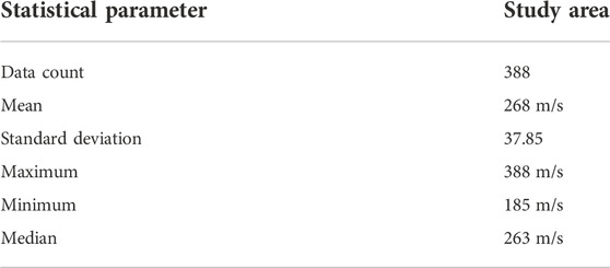
TABLE 1. Statistical characteristics of the known V_s30.

The empirical semi-variogram of V_s30 measurements is also computed to infer their spatial structure in the studied region. According to Goovaerts (1997), the empirical semi-variogram can be calculated as follow:

$\gamma \left(h\right)=\frac{1}{2N\left(h\right)}{\displaystyle \sum }_{\alpha =1}^{N\left(h\right)}{\left[Z\left(u_{\alpha }\right)-Z\left(u_{\alpha }+h\right)\right]}^2(10)$

In which, N(h)is the number of pairs of data with a distance of h.

To facilitate the incorporation of the semi-variogram into random field models, the empirical semi-variogram has to be fitted by a basic semi-variogram model or a linear combination of several basic semi-variogram models that are permissible. The three most commonly used models for fitting semi-variogram are the Exponential model, the Spherical model, and the Gaussian model (Liu et al., 2017a). Figure 5 plots the empirical semi-variogram model as well as the fitted exponential model of the form:

$\gamma \left(h\right)=\omega \left[1-\exp \left(-\frac{3h}{a}\right)\right]+\tau (11)$

FIGURE 5

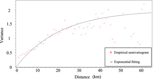
FIGURE 5. Empirical and fitted semi-variogram based on known V_s30 at measurement locations.

In which, h is the separation distance between any two points; a is the range, representing the distance at which the semi-variogram levels off. The fitted range of this study site is 19.67 km, and the nugget effect is neglected here for a better fit of the exponential model.

5 Random field realization of the Beijing area

With the statistical distribution of V_s30 values and the spatial structure of V_s30 at different locations, random field models are used to generate V_s30 maps of the Beijing area. A grid with the element size of 1 km*1 km is used, since the size of the study area is rectangular with a width of 44 km and a height of 68 km, so 2,992 elements are generated. The grid can be refined if it is necessary for future studies. Random field realization will be carried out based on this grid form, and finally, the corresponding V_s30 estimation value will be obtained in each element, which will be finally displayed in the form of a digital V_s30 map. The new map accounts for and preserves the site-specific shear wave velocity measurements and the soil spatial structure.

One time of V_s30 realization and its corresponding histogram is shown in Figure 6. The histogram shows that the simulation preserves the statistical characterizations of V_s30 inferred from the known V_s30 data.

FIGURE 6

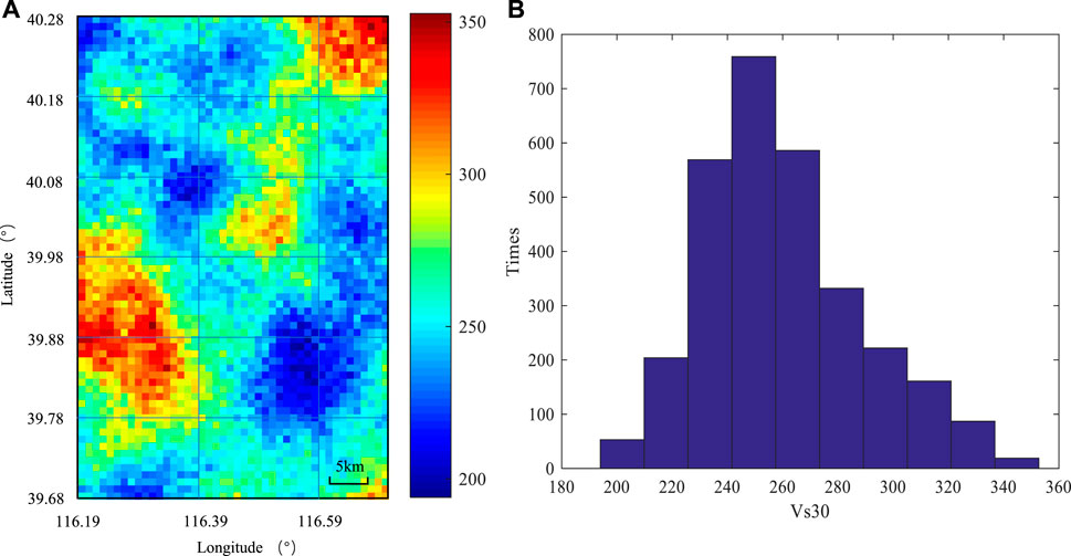
FIGURE 6. One-time random field realization of V_s30 in the Beijing area.(A) Map of V_s30 realization; (B) Histogram of V_s30.

A single random field simulation is only a random sampling based on a given distribution, and the result can not represent the true V_s30 value. Therefore, random field realization and the Monte Carlo sampling method are combined to carry out a large number of independent simulations. Coupling the random field model with Monte Carlo simulations, the expected V_s30 value across the Beijing area can be obtained, as well as its uncertainty distribution. Here, 1,000 times Monte Carlo simulations are operated and 1,000 independent maps can be generated. In other words, for the V_S30 of each 1 km*1 km element, 1,000 simulation calculations have been carried out. According to the simulation results of 1,000 times realizations, the mean value and coefficient of variation of the V_s30 prediction value can be obtained statistically for each element. Among them, the mean value of 1,000 simulations of each element represents the expected value of V_s30 of the element, and the variance and coefficient of variation represent the uncertainty of the shear wave (Crespo MariaJ. et al., 2022) velocity value at this point. By combining 2,992 elements, the V_s30 distribution and uncertainty distribution in the study area can be obtained. The expected V_s30 map is shown in Figure 7A. And it is averaged from these 1,000 times independent Monte Carlo simulations. An obvious trend in this map is that the overall soil quality in the study area is normal, ranging from 217.1623 m/s to 346.9406 m/s, the west-south part of this area has a relatively higher V_s30 value, which represents the Fang Shan hilly area. And the northeast corner also has high V_s30 values, which can be seen from the geology map as a hilly area too.

FIGURE 7

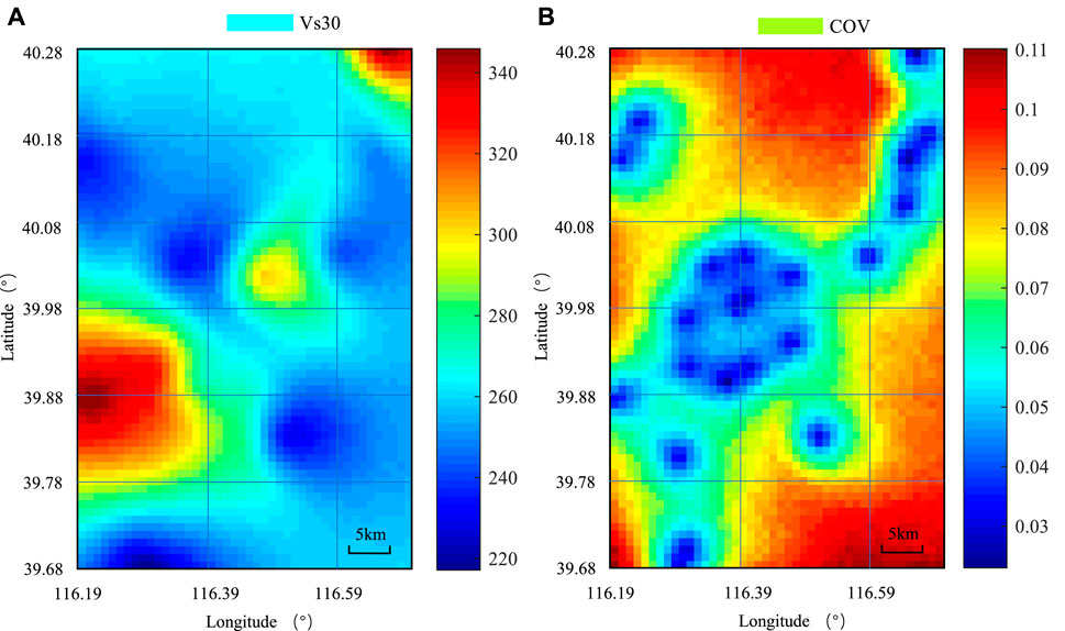
FIGURE 7. Expected V_s30 values and associated uncertainties (coefficient of variations) in the Beijing area. (A) Map of average V_s30; (B) Map of COV of V_s30.

Unlike the deterministic method, one of the strengths of the random field method is its ability to estimate the uncertainty distribution associated with the generated V_s30 map. Here, the coefficient of variation (COV) calculate from 1,000 independent Monte Carlo simulations at each location is calculated to quantify the uncertainties. The COV map is plotted in Figure 7B. As shown in the figure, the COVs are generally very small (ranging from 0.023 to 0.1102) and approach zero around locations with measurement data. And for the location without measured data, the COV value will be higher but still acceptable. It is worth noting that, in the (Crespo MJ. et al., 2022) simulation of this random field model, the study area is divided into 2,992 square elements, and the center point of each element is focused, the simulated V_s30 value of the center point is assigned to the whole square element. Hence, if the center point happens to be the measured data point, the COV of the cell is 0. If there are measured data points in the cell, but the measured data points are not exactly at the center point of the element, the simulated value of the cell will not be completely equal to the measured data value. But it will be very close, and the COV value of this cell will be very small (shown in dark blue in Figure 7B).

Since the V_s30 map has been generated, the accuracy of the prediction can be verified by using the testing data (30 measurements). According to the location of 30 testing data points, the corresponding element in the map can be found. Obtaining the corresponding V_s30 value of each element, cross-validation can be operated. The comparison results are shown in Figure 8. As can be seen from the figure, the prediction results are reasonable.

FIGURE 8

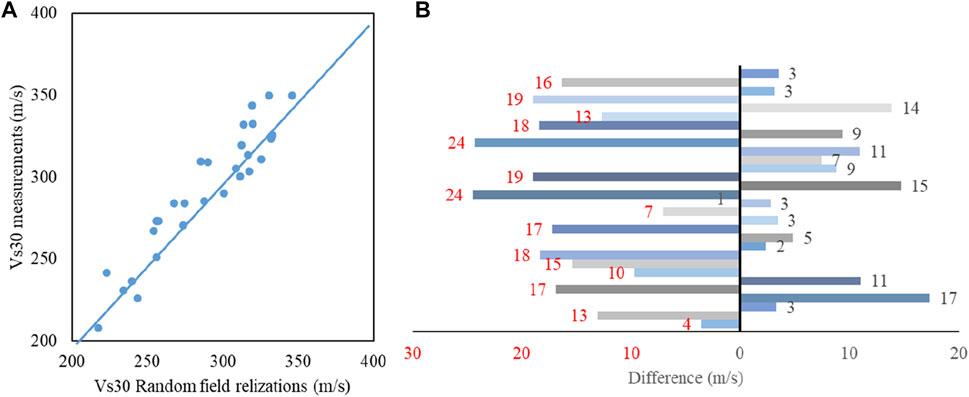
FIGURE 8. Cross-validation result of V_s30 realizations. (A) Comparison between random field realizations and measurements; (B) Differences of random field realizations and measurements.

Also, the inverse distance weighted method (IDW) is operated here to verify the result. Because both methods consider the variation of parameter values with spatial distance, hence, the two methods get similar results with an average difference of 13.95 m/s (Figure 9). The random field method describes spatial correlation by semi-variogram, which is more accurate than the inverse distance difference method. Moreover, the random field V_s30 map could provide both the expectation and uncertainty of a site parameter, which could be further integrated into the reliability analysis of the site response or earthquake disaster degree evaluation.

FIGURE 9

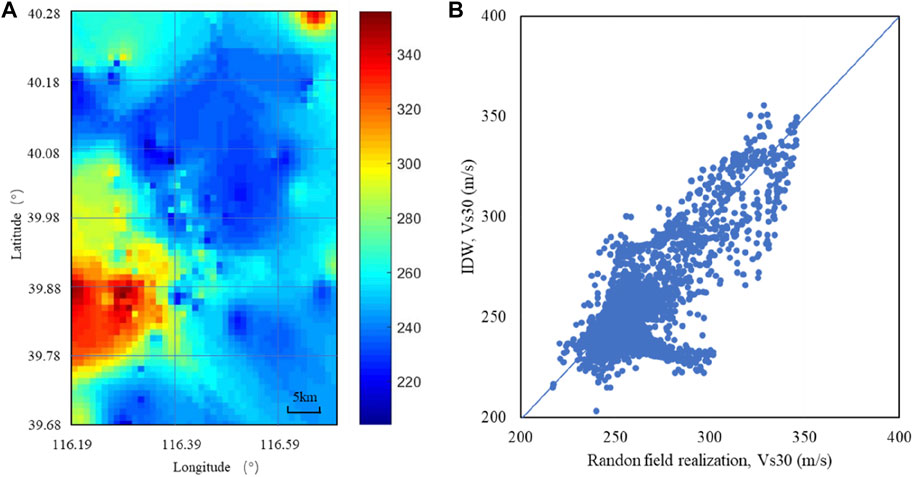
FIGURE 9. Comparison between IDW and Random field model: (A) V_s30 realizations calculated by IDW; (B) Comparison of results between two methods.

6 Effects of N

As described in Section 2, the unknown value Z_n at an unmeasured location can be drawn from the conditional normal distribution. Once Z_n is generated, it is inserted into the “previous” vector, upon which the “next” unknown value at another unsampled location will be generated. Hence, the “previous” vector is getting bigger during the simulation, it is unnecessary to use all of them to do the estimation. Therefore, it is necessary to define the “N” value (maximum number of previously generated elements to correlate to) when predicting value at unsampled locations, which will have a noticeable influence on the calculation results. After we set the value of N at the beginning of the estimation (e.g., 40), this value will keep constant for the whole simulation. This means when generating each unknown value at the unsampled location, only 40 “previous” data closest to this point will participate in the prediction, the nearest 40 data points are included in the covariance matrix calculation. And the values of other points will not have a direct impact on the prediction of this point. The principle behind this is that in geostatistical theory, the geotechnical or geological characteristics of the regional areas usually show spatial variability and spatial correlation, which means the soil parameters measured at each observation point are correlated with those at adjacent locations, and with the increase of distance, the correlation between the parameters decreases gradually. Therefore, five different values of N are selected, namely, 10, 20, 40, 60, and 80, and the simulation results are used to evaluate the influence of N.

Similar to Section 3, for each N value, the random field model is coupled with 1,000 times independent Monte Carlo simulations. So five sets of expected V_s30 values and their uncertainty distribution across the Beijing area are obtained (Figure 10).

FIGURE 10

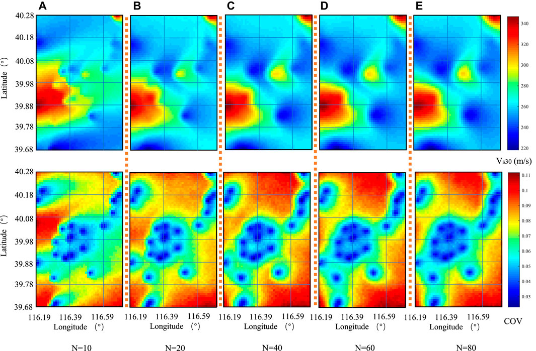
FIGURE 10. Expected V_s30 values and associated uncertainties in the Beijing area with different values of N. (A) N=10; (B) N=20; (C) N=40; (D) N=60; (E) N=80.

It can be seen from Figure 10 that with the increase of the N value (from 10 to 80), the prediction results gradually tend to be stable, and the change in the V_s30 map becomes invisible. Among them, for N changes from 10 to 40, the V_s30 distribution map has obvious changes, and in COV maps, the blue area expanded and the red area turns orange, which means the COV values turn smaller. And for N changes from 60 to 80, the predicted V_s30 distribution map is almost no different, similar to the COV maps. Detailed statistical results are listed in Table 2. It can be seen that the coefficient of variation (COV) is gradually decreasing with the increase of N, indicating that its prediction reliability is also gradually increasing. It is worth noting that for N changes from 10 to 60, the decreasing rate is large, and when N is larger than 60, the average COV value continues to decline, but the rate of decline is likely to remain steady.

TABLE 2

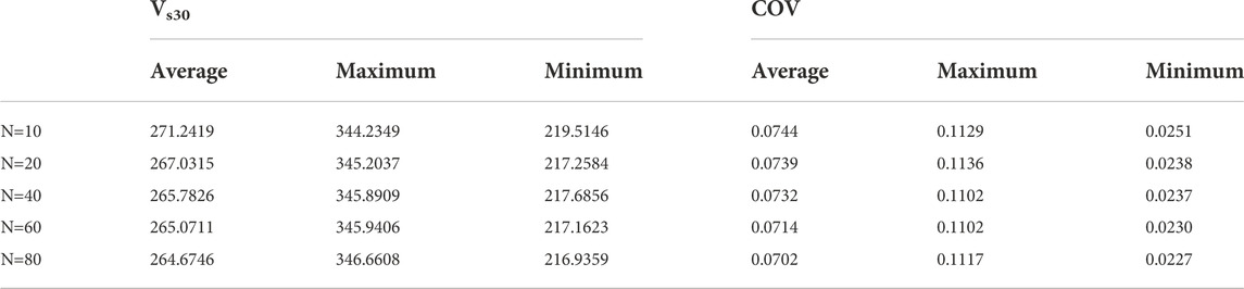
TABLE 2. Variability of V_s30 realizations under different N values.

The above observation shows that in the simulation process, the more “known values” are considered, the more accurate the results are (the lower the COV value is), and the improvement rate of its accuracy is gradually stable after reaching the peak with the increase of N. However, with the increase of the N value, the calculation matrix also increases, which increases the calculation workload and storage space required for calculation. Therefore, it is necessary to comprehensively consider the calculation efficiency and accuracy, and cannot blindly increase the N value. The appropriate N value can give us an appropriate result with a high calculation efficiency. So in this case, 60 is appropriate for this case study.

7 Conclusion

In this work, a random field prediction model of V_s30 is presented. And this prediction model is applied to map V_s30 and its uncertainty over the Beijing area. By operating statistical and geostatistical analysis of 388 measured bore data, the distribution and spatial variation of V_s30 are studied. Combining conditional sequence simulation technology and the Monte Carlo sampling method, the random field simulation of V_s30 at the city scale is carried out, and the two-dimensional V_s30 map and uncertainty distribution for the Beijing area are established. This new map can be applied to site classification and amplification factor characterization in the studied region in the future. Also, the effect of random filed model parameter N is tested. All the calculations and simulations in this paper are realized by self-made MATLAB code. In summary, it is found that:

1) V_s30 estimates over the entire studied region can be obtained using the random field model. The resulting map can give a detailed and reliable estimation of V_s30 at the unsampled location, meanwhile, the local measurement data are incorporated and preserved to make the new map consistent with the actual situation.

2) Coupled with the Monte Carlo simulation, the coefficient of variation (COV) can be easily obtained and is used to quantify the uncertainty distribution of V_s30 in the Beijing area. In general, COV is close to zero around locations with measured data, while COV gradually increases in areas without any measured V_s30 values.

3) The model parameter N (maximum number of previously generated elements to correlate to) will have a noticeable influence on the estimating V_s30 value at un-measured locations. The results show that with the increase of the N value, the prediction results gradually tend to be stable and the prediction reliability is gradually enhanced. However, the increase in the N value may cause an increase in the calculation workload and storage space required for calculation. Therefore, it is necessary to consider the calculation efficiency and accuracy comprehensively, and cannot blindly increase the N value.

4) Random field model and IDW method get similar results since both methods consider the variation of parameter values with spatial distance. However, the random field method describes spatial correlation by semi-variogram, which is more accurate than the inverse distance difference method. The presented methods are directly applicable to the site involving more complex property conditions. Moreover, the random field approach could provide both the expectation and uncertainty of a site parameter, which could be further integrated into the reliability analysis of the site response or earthquake disaster degree evaluation.

5) It is realized that estimation errors will be obtained when the geological conditions change abruptly (for example, from mountain to plain). So, it is necessary to use geological conditions to constrain the V_s30 estimation. And this will be the next step to improve this random field model by combining geological data and geotechnical data in V_s30 estimation.

Data availability statement

The datasets generated and analyzed during the current study are not publicly available but are available from the corresponding author on reasonable request. Requests to access the datasets should be directed to Wenxin Liu, wenxinl@zstu.edu.cn.

Author contributions

WL and YP conceived the presented idea. WL developed the theory and performed the computations. WL wrote the manuscript with support from YP and JW. All authors provided critical feedback and helped shape the research, analysis, and manuscript. YP supervised the project.

Funding

This work was supported by the National Natural Science Foundation of China (5210082052), the Zhejiang Provincial Natural Science Foundation (LQ22E080028), and the Science Foundation of Zhejiang Sci-Tech University (19052459-Y).

Acknowledgments

These financial supports are gratefully acknowledged.

Conflict of interest

The authors declare that the research was conducted in the absence of any commercial or financial relationships that could be construed as a potential conflict of interest.

Publisher’s note

All claims expressed in this article are solely those of the authors and do not necessarily represent those of their affiliated organizations, or those of the publisher, the editors and the reviewers. Any product that may be evaluated in this article, or claim that may be made by its manufacturer, is not guaranteed or endorsed by the publisher.

References

Ahdi, S. K., Stewart, J. P., Ancheta, T. D., Kwak, D. Y., and Mitra, D. (2017). Development of VS profile database and proxy-based models for VS 30 prediction in the Pacific Northwest region of North America. Bull. Seismol. Soc. Am. 107 (4), 1781–1801.

Google Scholar

Ancheta, T. D., Darragh, R., Stewart, J. P., Seyhan, E., Silva, W. J., Chiou, B. S. J., et al. (2013). PEER NGA-West2 database, PEER Report 2013/03. Berkeley, California: Pacific Earthquake Engineering Research Center.

Google Scholar

Badal, J., Dutta, Serón F., and Biswas, N. (2004). Three-dimensional imaging of shear wave velocity in the uppermost 30 m of the soil column in Anchorage, Alaska. Geophys. J. Int. 158 (3), 983–997. doi:10.1111/j.1365-246x.2004.02327.x

CrossRef Full Text | Google Scholar

Baise, L. G., Higgins, R. B., and Brankman, C. M. (2006). Liquefaction hazard mapping statistical and spatial characterization of susceptible units. J. Geotech. Geoenviron. Eng. 132 (6), 705–715. doi:10.1061/(asce)1090-0241(2006)132:6(705)

CrossRef Full Text | Google Scholar

Beijing Institute of Hydrogeology and Engineering Geology (1979). The bedrock geological map of Beijing plain. Biejing: Geological Publishing House. (in Chinese).

Google Scholar

Boore, D. M. (2004). Estimating s(30) (or NEHRP site Classes) from shallow velocity models (depths < 30 m). Bull. Seismol. Soc. Am. 94 (2), 591–597. doi:10.1785/0120030105

CrossRef Full Text | Google Scholar

Cai, X. M., Luan, Y. B., Guo, G. X., and Liang, Y. N. (2016). 3D Quaternary geological structure of Beijing plain. Geol. China 36 (5), 1021–1029. (in Chinese).

Google Scholar

Chen, G. X., Zhu, J., Qiang, M. Y., and Gong, W. P. (2018). Three-dimensional site characterization with borehole data-a case study of Suzhou area. Eng. Geol. 234, 65–82. doi:10.1016/j.enggeo.2017.12.019

CrossRef Full Text | Google Scholar

Ching, J., and Schweckendiek, T. (2021). State-of-the-art review of inherent variability and uncertainty in geotechnical properties and models. ISSMGE Tech. Comm., 304.

Google Scholar

Chiou, B. S. J., and Youngs, R. R. (2008). NGA model for average horizontal component of peak ground motion and response spectra, PEER Report 2008/09. Berkeley, California: Pacific Earthquake Engineering Research Center.

Google Scholar

Crespo, Maria J., Benjumea, Beatriz, Moratalla, José M., Lacoma, Luis, Albert, Macau, González, Álvaro, et al. (2022b). A proxy-based model for estimating V30 in the Iberian Peninsula. Soil Dyn. Earthq. Eng. 155, 107165. doi:10.1016/j.soildyn.2022.107165

CrossRef Full Text | Google Scholar

Crespo, M. J., Benjumea, B., Moratalla, J. M., Lacoma, L., Macau, A., Gonzalez, A., et al. (2022a). A proxy-based model for estimating VS30 in the Iberian Peninsula. Soil Dyn. Earthq. Eng. 155, 107165.

CrossRef Full Text | Google Scholar

DeGroot, D. J., and Baecher, G. B. (1993). Estimating autocovariance of in-situ soil properties. J. Geotech. Engrg. 119, 147–166. doi:10.1061/(asce)0733-9410(1993)119:1(147)

CrossRef Full Text | Google Scholar

Derras, B., Bard, P. Y., and Cotton, F. (2017). V_S30, slope, H800 and f0: Performance of various site-condition proxies in reducing ground-motion aleatory variability and predicting nonlinear site response. Earth Planets Space 69, 133. doi:10.1186/s40623-017-0718-z

CrossRef Full Text | Google Scholar

Derras, B., Bard, P. Y., Régnier, J., and Cadet, H. (2020). Non-linear modulation of site response: Sensitivity to various surface ground-motion intensity measures and site-condition proxies using a neural network approach. Eng. Geol. 269, 105500. doi:10.1016/j.enggeo.2020.105500

CrossRef Full Text | Google Scholar

Foster, K. M., Bradley, B. A., McGann, C. R., and Wotherspoon, L. M. (2019). A V_S30 map for New Zealand based on geologic and terrain proxy variables and field measurements. Earthq. Spectra 35 (4), 1865–1897. doi:10.1193/121118eqs281m

CrossRef Full Text | Google Scholar

Goovaerts, P. (1997). Geostatistics for natural resources evaluation. Duke: Oxford University Press on Demand.

Google Scholar

Hasancebi, N., and Ulusay, R. (2007). Empirical correlations between shear wave velocity and penetration resistance for ground shaking assessments. Bull. Eng. Geol. Environ. 66 (2), 203–213. doi:10.1007/s10064-006-0063-0

CrossRef Full Text | Google Scholar

Heath, D. C., Wald, D. J., Worden, C. B., Thompson, E. M., and Smoczyk, G. M. (2020). A global hybrid V_S30 map with a topographic slope–based default and regional map insets. Earthq. Spectra 36 (3), 1570–1584. doi:10.1177/8755293020911137

CrossRef Full Text | Google Scholar

Li, M., Rathje, E. M., Cox, B. R., and Yust, M. (2021). A Texas-specific VS 30 map incorporating geology and VS 30 observations. Earthq. Spectra 24, 87552930211033622.

CrossRef Full Text | Google Scholar

Liu, W. X., Chen, Q. S., Wang, C. F., Chen, G. X., and Juang, C. H. (2017b2017). Multiscale random field-based shear wave velocity mapping and site classification. Geo-Risk, 410–419.

CrossRef Full Text | Google Scholar

Liu, W. X., Chen, Q. S., Wang, C. F., Chen, G. X., and Juang, C. H. (2017a). Spatially correlated multiscale Vs30 mapping and a case study of the suzhou site. Eng. Geol. 220, 110–122. doi:10.1016/j.enggeo.2017.01.026

CrossRef Full Text | Google Scholar

Liu, W. X., Juang, C. H., Chen, Q. S., and Chen, G. X. (2021). Dynamic site response analysis in the face of uncertainty–an approach based on response surface method. Int. J. Numer. Anal. Methods Geomech. 45, 1854–1867. doi:10.1002/nag.3245

CrossRef Full Text | Google Scholar

Min, Z. Q., Wu, G., Jiang, Z. X., Liu, C. S., and Yang, Y. L. (1995). A Catalog of strong Historical earthquakes in China (from 2300 BC to 1911 AD). Beijing, China: Seismology Publishing House. (in Chinese).

Google Scholar

Parker, G. A., Harmon, J. A., Stewart, J. P., Hashash, Y. M. A., Kottke, A. R., Rathje, E. M., et al. (2017). Proxy-based V_S30 estimation in central and eastern North America. Bull. Seismol. Soc. Am. 107 (1), 117–131. doi:10.1785/0120160101

CrossRef Full Text | Google Scholar

Peng, H., Wu, Z., Wu, Y. M., Yu, S., Zhang, D., and Huang, W. (2011). Developing a prototype earthquake early warning system in the Beijing capital region. Seismol. Res. Lett. 82 (3), 394–403. doi:10.1785/gssrl.82.3.394

CrossRef Full Text | Google Scholar

Peng, Y., Wang, Z., Woolery, E. W., Lyu, Y., Carpenter, N. S., Fang, Y., et al. (2020). Ground-motion site effect in the Beijing metropolitan area. Eng. Geol. 266, 105395. doi:10.1016/j.enggeo.2019.105395

CrossRef Full Text | Google Scholar

Phoon, K. K., Cao, Z. J., Ji, J., Leung, Y. F., Najjar, S., Shuku, T., et al. (2022). Geotechnical uncertainty, modeling, and decision making. Soils Found. 62 (5), 101189. doi:10.1016/j.sandf.2022.101189

CrossRef Full Text | Google Scholar

Rahman, M., Kamal, A. S. M., and Siddiqua, S. (2018). Near-surface shear wave velocity estimation and V_s30 mapping for Dhaka City, Bangladesh. Nat. Hazards (Dordr). 92 (3), 1687–1715. doi:10.1007/s11069-018-3266-3

CrossRef Full Text | Google Scholar

Raptakis, D. G., Anastasiadis, S. A. J., Pitilakis, K. D., and Lontzetidis, K. S. (1995). “Shear wave velocities and damping of Greek natural soils,” in Proceedings of 10th European Conference of earthquake engineering (Vienna, 477–482.

Google Scholar

Seed, H. B., and Idriss, I. M. (1981). Evaluation of liquefaction potential sand deposits based on observation of performance in previous earthquakes. InASCE Natl. Conv. (MO), 481–544.

Google Scholar

Stewart, J. P., and Afshari, K. (2021). Epistemic uncertainty in site response as derived from one-dimensional ground response analyses. J. Geotech. Geoenviron. Eng. 147 (1), 04020146. doi:10.1061/(asce)gt.1943-5606.0002402

CrossRef Full Text | Google Scholar

Stewart, J. P., Klimis, N., Savvaidis, A., Theodoulidis, N., Zargli, E., Athanasopoulos, G., et al. (2014). Compilation of a local VS profile database and its application for inference of VS30 from geologic- and terrain-based proxies. Bull. Seismol. Soc. Am. 104 (6), 2827–2841. doi:10.1785/0120130331

CrossRef Full Text | Google Scholar

Thompson, E. M., Baise, L. G., and Kayen, R. E. (2007). Spatial correlation of shear-wave velocity in the san Francisco Bay area sediments. Soil Dyn. Earthq. Eng. 27 (2), 144–152. doi:10.1016/j.soildyn.2006.05.004

CrossRef Full Text | Google Scholar

Wald, D. J., and Allen, T. I. (2007). Topographic slope as a proxy for seismic site conditions and amplification. Bull. Seismol. Soc. Am. 97 (5), 1379–1395. doi:10.1785/0120060267

CrossRef Full Text | Google Scholar

Wald, D. J., McWhirter, L., Thompson, E., and Hering, A. S. (2011). “A new strategy for developing VS30 maps,” in Proc. 4th Int. Effects of surface geology on seismic motion Symp.

Google Scholar

Wang, J. H., and Han, X. (2012). Preliminary study on Tertiary engineering geological conditions in Beijing Plain area. J. Eng. Geol. 20 (5), 682–686. (in Chinese).

Google Scholar

Wang, S. Y., Wu, G., and Shi, Z. L. (1999). A Catalog of modern earthquakes in China (1912–1990). Beijing, China: China Science and Technology Press. (in Chinese).

Google Scholar

Wills, C. J., Gutierrez, C. I., Perez, F. G., and Branum, D. M. (2015). A next generation V_S30 map for California based on geology and topography. Bull. Seismol. Soc. Am. 105 (6), 3083–3091. doi:10.1785/0120150105

CrossRef Full Text | Google Scholar

Wride, C. E., Robertson, P. K., Biggar, R. G., Campanella, R. G., Hofmann, B. A., Hughes, J. M. O., et al. (2000). Interpretation of in situ test results from the CANLEX sites. Can. Geotech. J. 37 (3), 505–529. doi:10.1139/t00-044

CrossRef Full Text | Google Scholar

Xie, J. J., Zimmaro, P., Li, X. J., Wen, Z., and Song, Y. S. (2016). V_S30 empirical prediction relationships based on a new soil-profile database for the Beijing Plain Area, China. Bull. Seismol. Soc. Am. 106 (6), 2843–2854. doi:10.1785/0120160053

CrossRef Full Text | Google Scholar

Yong, A., Martin, A., Stokoe, K., and Diehl, J. (2013). ARRA-funded VS30 measurements using multi-technique approach at strong-motion stations in California and central-eastern United States (No. 2013-1102). U. S. Geol. Surv. 47, 5765.

Google Scholar

Yuan, H., Gao, X., and Qi, W. (2019). Modeling the fine-scale spatiotemporal pattern of earthquake casualties in cities: Application to Haidian District, Beijing. Int. J. disaster risk Reduct. 34, 412–422. doi:10.1016/j.ijdrr.2018.12.010

CrossRef Full Text | Google Scholar

Zhang, J. Z., Huang, H. W., Zhang, D. M., Phoon, K. K., Liu, Z. Q., and Tang, C. (2021). Quantitative evaluation of geological uncertainty and its influence on tunnel structural performance using improved coupled Markov chain. Acta Geotech. 16 (11), 3709–3724. doi:10.1007/s11440-021-01287-6

CrossRef Full Text | Google Scholar