 Rong Mianshui
 Fu Li-Yun
 Sánchez-Sesma Francisco José
 Sun Weijia
94% of researchers rate our articles as excellent or good
Learn more about the work of our research integrity team to safeguard the quality of each article we publish.
Find out more
ORIGINAL RESEARCH article
Front. Earth Sci., 08 August 2022
Sec. Structural Geology and Tectonics
Volume 10 - 2022 | https://doi.org/10.3389/feart.2022.948697
This article is part of the Research TopicMeasuring, Modeling and Predicting the Seismic Site EffectView all 20 articles
Joint inversion of horizontal-to-vertical spectral ratios (HVSRs) and dispersion curves (DCs) from seismic noise recordings has been extensively used to overcome the lack of inversion uniqueness in the noise-based HVSR (NHV) or DC inversions alone. Earthquake recordings contain information about the structural properties of sedimentary layers and provide body-wave data complementary to seismic noise recordings to estimate site velocity structures, particularly in the high-frequency band. We propose a joint inversion of the Rayleigh wave DC obtained from array measurements and earthquake-based HVSR (EHV). The EHV is derived from earthquake motions rather than from microtremors based on the diffuse-field theory of plane waves. We investigated the complementarity of EHV and surface-wave DC in the joint inversion through sensitivity analyses. The DC is sensitive to bedrock shear-wave velocities in the low-frequency range and is supplemented to some degree by the EHV in the high-frequency range. The EHV is more sensitive to sediment thicknesses almost over the entire frequency range. The joint inversion is implemented by a hybrid global optimization scheme that combines genetic algorithm (GA) and simulated annealing (SA) to avoid premature convergence in the GA. The sensitivity of inversion parameters was tested to demonstrate that the P- and S-wave velocities and thicknesses of soil layers are the dominant parameters influencing EHV and DC responses. The proposed method was validated by using synthetic models to compare the joint inversion with EHV or DC inversions alone. The joint inversion was applied to the Garner Valley Downhole Array (GVDA) data for identifying the velocity structures of the site based on earthquake and noise observations. The inversion results for the P- and S-wave velocities and thicknesses of soil layers strongly suggest that the joint inversion is an efficient method to estimate site velocity structures.
It is well known that the site effect can affect the characteristics of strong ground motions and consequently influence the distribution of damage during earthquakes. The shear-wave velocity (VS) and thickness of soil layers are essential parameters for the quantitative evaluation of site effects. Empirical methods based on surface seismic recordings have been widely used to study site effects for estimating the Vs. profile. Among these methods, the horizontal-to-vertical spectral ratio (HVSR) proposed by Nakamura (1989) typically has a conspicuous peak that is a good estimator of dominant frequency and soon became popular because of its economy and effectiveness. Moreover, the HVSR has been widely used to estimate velocity structures from observed earthquake ground motions and microtremor measurements (Kawase, et al., 2018). In this study, to make full use of the available earthquake and noise measurement data, we propose a joint inversion of earthquake-based HVSR (hereafter, EHV) and phase velocity dispersion curve (hereafter, DC), where the HVSR is derived from earthquake motions rather than from microtremors based on the diffuse-field theory of plane waves (Kawase, et al., 2011).
Velocity profiles (particularly, the shear-wave velocity one) are often retrieved from surface recording data of passive sources, such as seismic ambient noise. The pioneering SPAC method (Aki, 1957) has been widely used. This approach has been rapidly developed through the continuous accumulation of observation data and has gained wide interest owing to its cost effectiveness. The shear-wave velocity profile can be obtained by the inversion of Rayleigh wave DCs (Aki, 1957; Louie, 2001; Wathelet, 2005; Gouedard et al., 2008; Tada et al., 2009) or by the combined inversion of the DC and ellipticity of Rayleigh waves (e.g., Scherbaum et al., 2003). Generally, the Rayleigh waves DC are derived from microtremors recorded by several instruments; therefore, the detecting instruments should form an array with a certain scale. In contrast, the HVSR inversion based on single-station recordings is much more convenient. The HVSR inversion methods can be classified into four typical categories: (1) HVSR based on the Rayleigh wave ellipticity (Fäh et al., 2001; Sherbaum et al., 2003), (2) HVSR based on the contributions of Rayleigh and Love waves (Arai and Tokimatsu, 2004), (3) HVSR based on the contribution of body waves (Herak, 2008; Bignardi et al., 2016), and (4) HVSR based on the contribution of the body and surface waves according to the diffuse wave field theory (Kawase et al., 2011; Sánchez Sesma et al., 2011; Nagashima et al., 2014). Although the HVSR inversion method is advanced, its use is hampered by the phenomenon of the non-uniqueness of the solution as demonstrated by Picozzi et al. (2005) and Picozzi and Albarello (2007).
To overcome this problem, Scherbaum et al. (2003) proposed a joint inversion of HVSR and phase velocity dispersion to determine the soil profile. Parolai et al. (2005) and Picozzi et al. (2005) performed joint inversions of the phase velocity dispersion and HVSR curves. In these joint inversions, the HVSR and DCs were obtained from ambient noise observations. Although the forward modeling calculation of noise-based HVSR (NHV) improved by García-Jerez et al. (2016) and Pina-Flores et al. (2017) is more efficient than the conventional wavenumber-integration schemes, the inversion still needs thousands of iterations and each is time-consuming for general applications. In contrast, the EHV can be easily calculated by considering only the single-wavenumber contribution of body waves (Kawase et al., 2018).
In recent years, several studies proved that the one-dimensional (1D) velocity structure could be obtained through the inversion of HVSR from earthquake motions (Kawase et al., 2011; Nagashima et al., 2014). Commonly the S-wave window of earthquake motion is adopted to calculate the EHV, under this situation, the EHV inversion is dominated by body-wave contributions. Therefore, it is natural to combine the EHV with phase velocity DCs for integrating surface- and body-wave components and they both are modeled from the layered system properties under scrutiny. The joint inversion can add extra constraints to reduce the non-uniqueness of the solutions associated with the single EHV inversion. Therefore, this strategy improves the efficiency and accuracy of the inversion for soil profiles. For an area where EHV can be easily obtained, the joint inversion of EHV and DC is especially appropriate and does not impose any additional computational cost on collecting earthquake motion data. For example, many strong ground motion stations in western China offer abundant earthquake recordings, but soil profiles are not available. With the joint inversion method, these ground motions can be used to estimate site velocity structures if some small-scale noise arrays are set up to extract DCs from microtremor measurements. To the best of our knowledge, such a joint inversion implementation has not been reported yet.
From the viewpoint of the inversion algorithm, the genetic algorithm (GA) has been widely used to deal with sundry HVSR measurements (Scherbaum et al., 2003; Parolai et al., 2005; Picozzi et al., 2005). However, during the inversion process, the algorithm tends to stall away from the global optimal solution. This phenomenon is called premature convergence (Mosegaard and Sambridge, 2002). To overcome this problem, often different optimization methods are combined (Santos et al., 2005); for example, hybrid GA and linearized (LIN) algorithms (Picozzi and Albarello, 2007) and hybrid simulated annealing (SA) and GA (Cui, 2004). The simulation shows that the premature convergence of GA and the search inefficiency of SA can be improved simultaneously in the hybrid scheme. The combinational strategy of SA and GA was applied to the inversion of EHV (Rong et al., 2018). In this study, the global optimization scheme of hybrid SA and GA was applied to the proposed joint inversion.
In this study, we conducted the joint inversion of EHV and phase velocity dispersion for site velocity structures. The EHV is obtained based on the diffuse-field theory for plane waves. In order to construct neatly the synthetic 1D diffuse illumination. Thus, only the S-wave part (which certainly includes other waves) is used to calculate EHV. The DC derived from array measurements is an essential constraint to the EHV. To delve into the effectiveness of the combined application of these two different methods, we investigated their complementarity in the inversion. The NHV is a byproduct of these noise measurements. The benefit of the joint inversion using earthquake data to determine the HVSR comes from the fast forward computations. …To examine our joint inversion in detail, we investigated the complementarity of EHV and surface-wave DC through sensitivity analyses. The inversion was implemented using a global optimization algorithm of hybrid GA and SA algorithms. We discussed the sensitivity of various parameters (S- and P-wave velocities, thickness, and density) to the inversion. We validated the proposed method by using a synthetic example to compare the performances of the joint inversion of NHV and DC with those of EHV or DC inversions alone. Finally, the joint inversion was applied to the Garner Valley Downhole Array (GVDA) data for identifying site velocity structures.
Both single-station HVSR and phase velocity DCs can capture the mechanical and structural properties of sedimentary layers. The combined application of the two datasets can constrain the Vs. structure better. The proposed joint inversion includes two steps, namely, (1) the forward calculation of EHV and DCs, and (2) the global optimization for searching the best structural model by the hybrid GA and SA algorithms.
Arai and Tokimatsu (2004) improved the forward calculation of HVSR from microtremor measurements by considering the higher modes. Based on the diffuse-field theory, Sánchez-Sesma et al. (2011) linked the average measurements of HVSR to the intrinsic property of the media by regarding the power spectrum of measurements as proportional to the directional energy densities. This simplifies the forward calculation considering the full-wave HVSR as proportional to the imaginary part of the Green’s function (Wu et al., 2017). …To extend the diffuse-field theory to earthquake records, Kawase et al. (2011) showed that for body waves incident to a 1D layered structure, the EHV can be calculated as
where
We used Eq. 1 to calculate the EHV curves in the proposed joint inversion. Figure 1A presents the theoretical EHV of the GVDA site. The measured profile data (Bonilla et al., 2002) are listed in Table 1. The model parameters in the table include the P-wave velocity (VP), S-wave velocity (Vs), density (ρ), and thickness (h) for individual layers. Based on these parameters that define a 1D model whose properties vary with the depth, we calculated the theoretical DC using “gpdc” program, a routine in the GEOPSY software package (Wathelet et al., 2020). Figure 1B shows the resulting theoretical DC for the GVDA array site. The calculation of experimental DC was made from microtremor measurements in and array using the frequency-wavenumber method (Wathelet, 2005).

FIGURE 1. Forward calculation of the theoretical EHV (A) and DC (B) for the GVDA site (Bonilla et al., 2002).
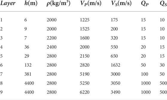
TABLE 1. Measured model of GVDA site (Bonilla et al., 2002).
Since the aim of the inversion is to retrieve a 1D subsurface structure, we need a criterion to decide which set of simulated curves best reproduces the experimental data. Hence, we introduce an objective function that is a positive, real valued function of the subsurface parameters. The objective function becomes important in the proposed joint inversion because EHV and DC are physically different, have nonidentical dominant frequencies, and are related to subsurface velocity profiles in distinct ways and to different degrees. A reasonable objective function is a good representation of the impacts of different types of data on the inversion.
The problem of determining underground velocity structures by the joint inversion of EHV and DC can be simplified as the problem of finding the global minimum value of the objective function that relates soil parameters to EHV and DC curves. Following Parolai et al. (2005), we defined the objective function as
where ΦDC and ΦHV are the objective functions for dispersion and EHV curves, respectively, and P= (x1,x2,x3, … ,xN)T is the parameter vector of the model with N soil layers.
Similar to Lawrence and Wiens (2004), the objective functions ΦDC and ΦHV in Eq. 2 can be expressed as
where
In this study, we incorporated the SA into the GA in an attempt to seek the global minimum of the multiple extreme value problems. The hybrid global optimization method considers the effects of S- and P-wave velocities, thicknesses, and densities on the EHV and DC curves.
The global optimization method of hybrid GA and SA (Rong et al., 2018), which was originally developed for EHV inversions, was modified to consider the EHV and DCs simultaneously for the joint inversion. In this hybrid implementation, the premature convergence of GA is avoided by the SA annealing operation and the search inefficiency of SA is improved by the GA global optimizing operation.
We denote the set of parameters of the ith layer by pi = (VSi,VPi,hi,ρi), with i = 1,2,3, … ,N. Some background parameters should be set in advance. These parameters include the genetic population size (M), variable dimension (maximum number of variables considered in the inversion), binary digits, initial temperature T0 for SA, and the iteration number of generations (L) at a certain temperature.
The hybrid GA and SA method relies mainly on the GA and is supplemented by the SA. We first initialize the genetic population model by calculating its objective function and every individual relative fitness. Each individual in the population model is denoted by a string of binary codes with 0 and 1. Then the objective functions for individuals are calculated and ranked. According to the ranking of objective functions, the fitness value are normalized and assigned as values between −2 and 2.
The fitness value describes the superiority or inferiority of individuals. It is used to determine the next genetic operation: selection, crossover, or mutation. The initial population can be evolved into the next generation. The larger the fitness of an individual, the higher is the probability that the individual will be reproduced and passed down into the next generation.
The SA operation is introduced to reduce the premature convergence of the GA. In this operation, we compare the objective functions of “child” individuals (
where c is the temperature attenuation coefficient, which is typically a constant less than one.
The computational flow for the hybrid implementation of the GA and SA is principally based on the GA. Figure 2 depicts the flow chart of the inversion with the following main steps.
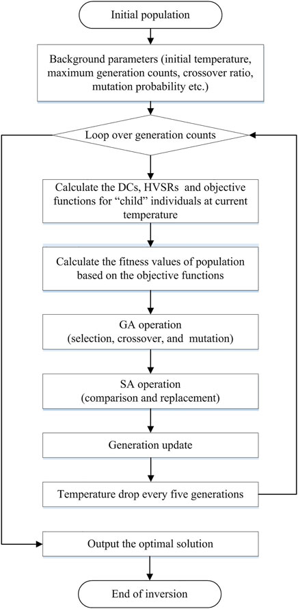
FIGURE 2. Flow chart of the proposed joint inversion.
Step 1. Create the initial population.
Step 2. Set up the background parameters—the initial temperature, maximum generation counts, crossover ratio, mutation probability, etc.
Step 3. Loop over the generation counts to calculate the DCs, EHVs, and objective functions of child individuals at the current temperature; then, compute the fitness value of the population based on the objective functions.
Step 4. Perform the GA operations of each generation loop to conduct selection, crossover, and mutation.
Step 5. Perform the SA operations of each generation loop to compare the objective functions of
Step 6. Output the optimal solution to end the inversion process.
The joint inversion by combining Rayleigh wave DC and EHV is based on their complementarity in the inversion. We investigated the complementarity and provided some supplementation through sensitivity analyses by using a simple model. The use of multiple parameters (VP, VS, h, and ρ) makes the model space of inversion very large, significantly reducing the efficiency of calculations. The sensitivity analysis of inversion parameters can reduce the spatial dimension of inversion problems to some extent.
Following Arai and Tokimatsu (2004), we defined the following absolute value of the nondimensional partial derivative of inversion parameters as the sensitivity of inversion
where
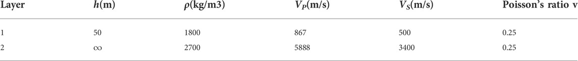
TABLE 2. A simplified soil structure (Kawase et al., 2011).
In the joint inversion, parameters such as thicknesses, S- and P-wave velocities, and densities affect the EHV, NHV, and DC curves in distinct ways and to different degrees. The computation of NHV was proposed by Sánchez-Sesma et al. (2011) and corresponds to the square root of the spectral ratio of the horizontal components of Green’s function to that of the vertical counterpart. Based on the soil model in Table 2, we calculated
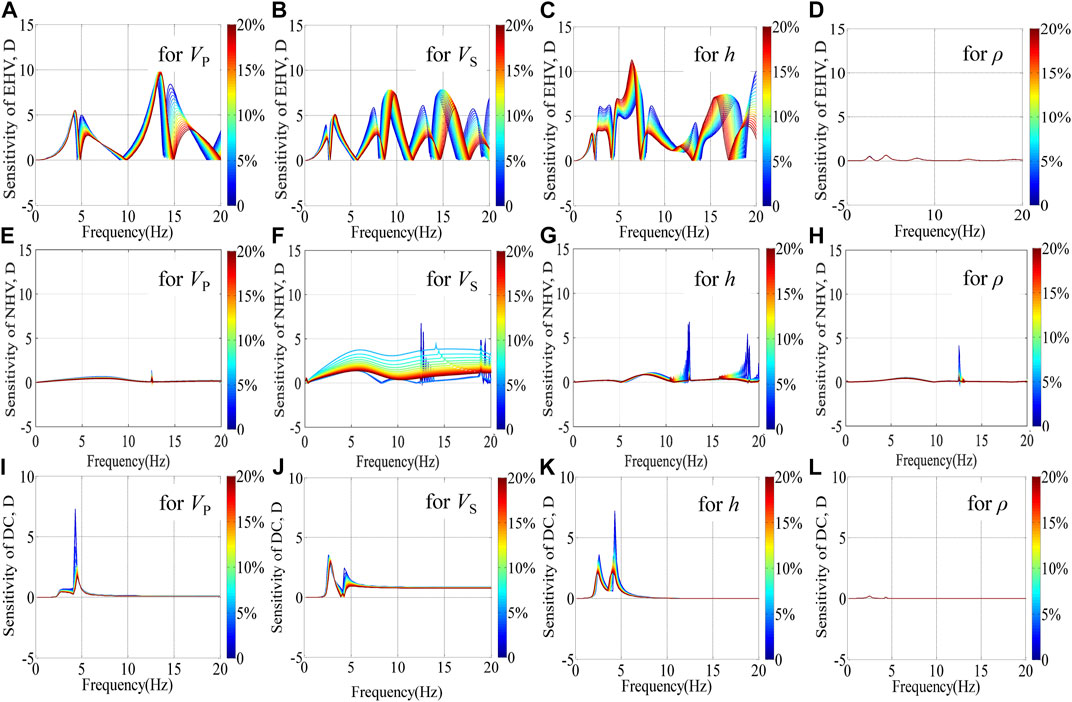
FIGURE 3. The sensitivity of different parameters to the EHV, NHV or DC, (A) VP to the EHV, (B) VS to the EHV, (C) h to the EHV, (D) ρ to the EHV, (E) VP to the NHV, (F) VS to the NHV, (G) h to the NHV, (H) ρ to the NHV, (I) VP to the DC, (J) VS. to the DC, (K) h to the DC, (L) ρ to the DC. The color bar is calibrated in terms of the variability of parameters. We consider 0–20% for the variation range of parameters.
The HVSR can be approximately interpreted as a receiver function in the frequency domain (Yu et al., 2017) having in mind that neither the azimuth nor the incidence angle are known. We only consider it is sensitive to impedance contrasts (i.e., strata interfaces), whereas the DC is sensitive to shear-wave velocities. Parolai et al. (2005) found that the joint inversion of HVSRs and DCs from seismic noise recordings can reduce the problem of trade-off between the velocity and thickness of layers. Picozzi et al. (2005) further showed that the bedrock S-wave velocity can be well constrained through this joint inversion. However, the HVSR in the previous joint inversions were based on seismic noise recordings and therefore based on the assumption of surface waves. However, as we know, NHV and EHV are quite distinct in terms of their frequency contents and propagation paths and modes because of the differences between surface and body waves. In addition, to the best of our knowledge, the complementarity of EHV and surface-wave DC in inverse problems has not be specifically clarified until now.
As a preliminary attempt in this regard, we extended sensitivity analyses using equation (5) to identify the complementarity of EHV and DC using the model detailed in Table 2. We tested the sensitivity of EHV, NHV, and surface-wave DC separately to the bedrock S-wave velocities and sediment thicknesses. We conducted two groups of tests. For the first group, we fixed the sediment thickness at 20 m with the other relevant properties as listed in Table 2, and then, we changed the bedrock S-wave velocity from 667 to 3333 m/s as the corresponding P-wave velocity was varied from 1155 to 5773 m/s to maintain the Poisson’s ratio of the bedrock at 0.25. The sediment–bedrock impedance contrast (IC) varied correspondingly from 2 to 10. We emphasize that because the sediment velocities (see Table 2) and sediment and bedrock densities were fixed, the sediment–bedrock IC values mainly reflect the change in the bedrock S-wave velocities. The fundamental resonance frequency (f0) used in these tests was 6.25 Hz because only impedance contrasts were considered. For the second group, we fixed the bedrock S-wave velocity by setting IC = 2 and then changed the sediment thickness from h0 to 5h0 with h0 = 20 m.
Figure 4 shows the resultant sensitivity of the EHV, NHV, and DC to S-wave velocities (by fixing h = 20 m) and sediment thicknesses (by fixing IC = 2). We considered a 5% variation range for velocities and thicknesses. The EHV, NHV, and DC exhibited different sensitivities for different frequency ranges. The EHV is more sensitive to the variation in sediment thicknesses almost throughout the frequency range, especially in the high-frequency range (>10 Hz). As expected, it is less sensitive to bedrock S-wave velocities. On the other hand, the DC is more sensitive to changes in the bedrock shear-wave velocities in the low-frequency range (<10 Hz), and less sensitive to sediment thicknesses. The NHV exhibits has similar sensitivity characteristics as the DC; for example, the NHV is also more sensitive to changes in the bedrock shear-wave velocities in the frequency range less than 10 Hz and less sensitive to sediment thicknesses. This is because NHV and DC are derived from microtremor measurements, which mainly consist of surface waves, so that the peaks associated with higher modes are not be as prominent as those in the case of EHV. The EHV is derived from earthquake ground motions, which mainly consist of upwardly propagating plain body waves, and hence, the higher mode resonances can be seen at high frequencies. This result indicates that from the viewpoint of sensitive frequency range, the joint inversion of the EHV and DC is more complementary than that of the NHV and DC. The former method can exploit the complementarity of the EHV and DC to achieve a reliable inversion for bedrock shear-wave velocities and sediment thicknesses.
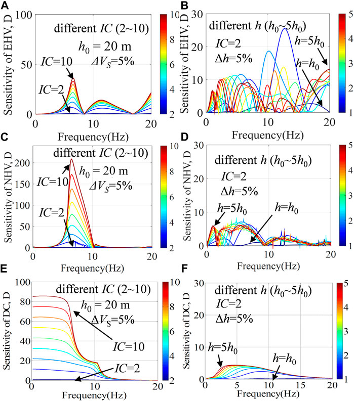
FIGURE 4. The sensitivity of bedrock S-wave velocities (A), and sediment thicknesses (B) to the EHV; The sensitivity of bedrock S-wave velocities (C), and sediment thicknesses (D) to the NHV; The sensitivity of bedrock S-wave velocities (E), and sediment thicknesses (F) to the DC. For the (A) (C), and (E), we fix the sediment thickness h = 20 m with the other relevant properties listed in Table 2, and then change the bedrock S-wave velocity to make the sediment-bedrock impedance contrast IC = 2–10, with the color bar calibrated in terms of the sediment-bedrock impedance contrast. For the (B), (D) and (F), we fix the bedrock S-wave velocity by setting IC = 2, and then change the sediment thickness from h0 to 5h0 (h0 = 20 m), with the color bar calibrated in terms of sediment thicknesses for a variation range of 5%.
Figure 4 clearly shows that the contribution of the EHV covers the whole frequency range and the contribution of the DC mainly lies in low and middle frequencies. It implies that the joint inversion of EHV and DC has complementarity from the aspect of frequency. However, the joint inversion for bedrock S-wave velocities does not appear as reliable in the middle-to-high-frequency band because there is almost no contribution of the DC. We need to identify the contribution of the EHV in this frequency band. For this purpose, the first group of tests, described previously, to test the sensitivity of the EHV and DC to different sediment–bedrock ICs for a sediment thickness h = 20 m and a fundamental resonance frequency f0 = 6.25 Hz, is extended to different sediment thicknesses (h = 25, 50, and 100 m) and corresponding predominant frequencies (f0 = 5, 2.5, and 1.25 Hz, respectively).
Figure 5 shows the resultant sensitivity of the EHV and DC to bedrock S-wave velocities for three fixed predominant frequency–sediment thickness pairs: 5 Hz and 25 m; 2.5 Hz and 50 m; and 1.25 Hz and 100 m. We see that the EHV and DC curves exhibit great changes for different parameter pairs. The responses of the DC to bedrock S-wave velocities mainly lie in the frequency range less than 2f0, whereas the EHV is sensitive to bedrock S-wave velocities over a wide range of frequencies around f0 and beyond. That is, the frequency complementarity of the EHV and DC can assure the joint inversion for bedrock shear-wave velocities.
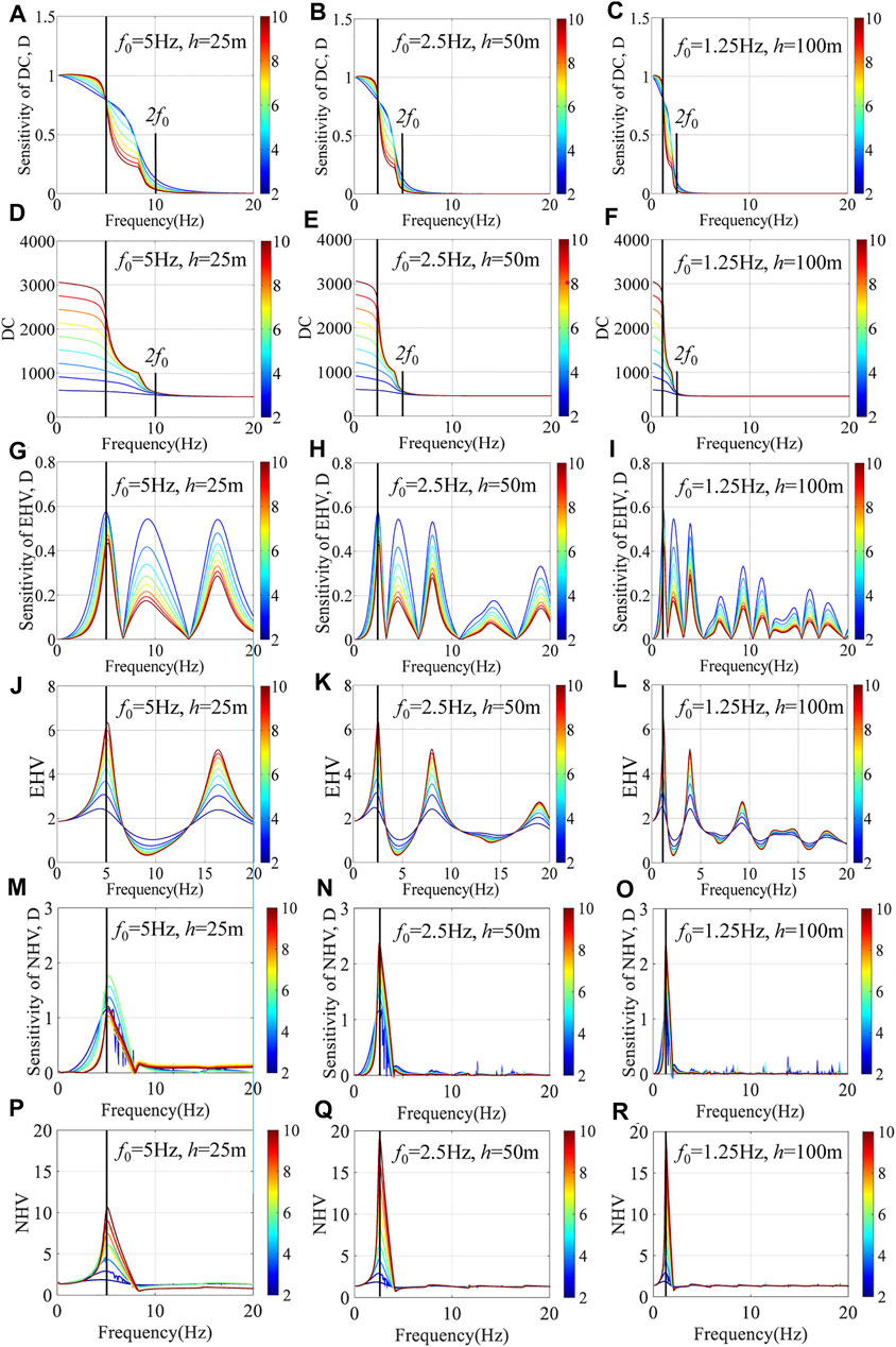
FIGURE 5. The sensitivity of the DC, EHV and NHV to bedrock S-wave velocities, along with the corresponding DC, EHV and NHV curves. The left (A,D,G,J,M,P), middle (B,E,H,K,N,Q), and right (C,F,I,L,O,R) panels result from the numerical experiments with three fixed parameter pairs of predominant frequency and sediment thickness: (5 Hz, 25 m) (2.5 Hz, 50 m), and (1.25 Hz, 100 m). The color bar is calibrated in terms of the sediment-bedrock impedance contrast IC = 2–10.
We considered the example of the GVDA site to validate the proposed joint inversion. The detailed velocity model for this site has been studied widely (e.g. Gibbs, 1989; Pecker and Mohammadioun, 1993; Theodulidis et al., 1996). As per the details in Table 1, the model was improved by the best fitting of the time-domain simulations and observed data (Bonilla et al., 2002). It has been widely used as a standard model to test various inversion algorithms.
The theoretical EHV and DC curves of the GVDA model are shown in Figure 1. Gaussian noise with a signal-to-noise ratio of 30 dB were added to these theoretical curves to test the robustness of the joint inversion algorithm. The resulting target curves are shown as red curves in Figures 6A,B. Although no initial model is required for our hybrid global optimization inversion, it is preferable to have one to constrain the search range of parameters. In this synthetic case, the P- and S-wave velocities and layer thicknesses were used as the unknown parameters based on the parameter sensitivity analysis described in the previous section. The bottommost layer was used as the bedrock with its parameters fixed in the inversion. The P- and S-wave velocities (VP0 and VS0) and thickness (h0) of the measured GVDA model (listed in Table 1) were used to determine the search ranges of all the model parameters. For example, the search ranges of each layer were set as (0.5–1.5) VP0 (0.5–1.5) VS0, and (0.5–1.5) h0 for P- and S-wave velocities and thickness, respectively. Details of the resultant initial model for inversion are listed in Table 3.
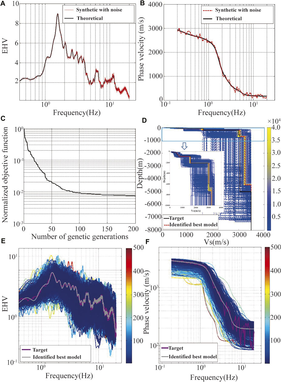
FIGURE 6. Verification of joint inversion of EHV and DC by the noise-contaminated synthetic case with the GVDA model. (A) The theoretical (solid line) and noise-contaminated synthetic (red dashed line) HVSRs of the GVDA mode. (B) The theoretical (solid line) and noise-contaminated synthetic (red dashed line) DCs of the GVDA mode. (C) Iterative convergence curve by objective functions versus generation numbers. (D) Inverted velocity profiles. the color bar is calibrated in terms of the order of appearance of the individuals. (E) and (F) The corresponding HVSR and DC curves of all the iterative models colored in terms of the value of objective functions which converge to the target curves (purple lines) with decreasing objective functions.
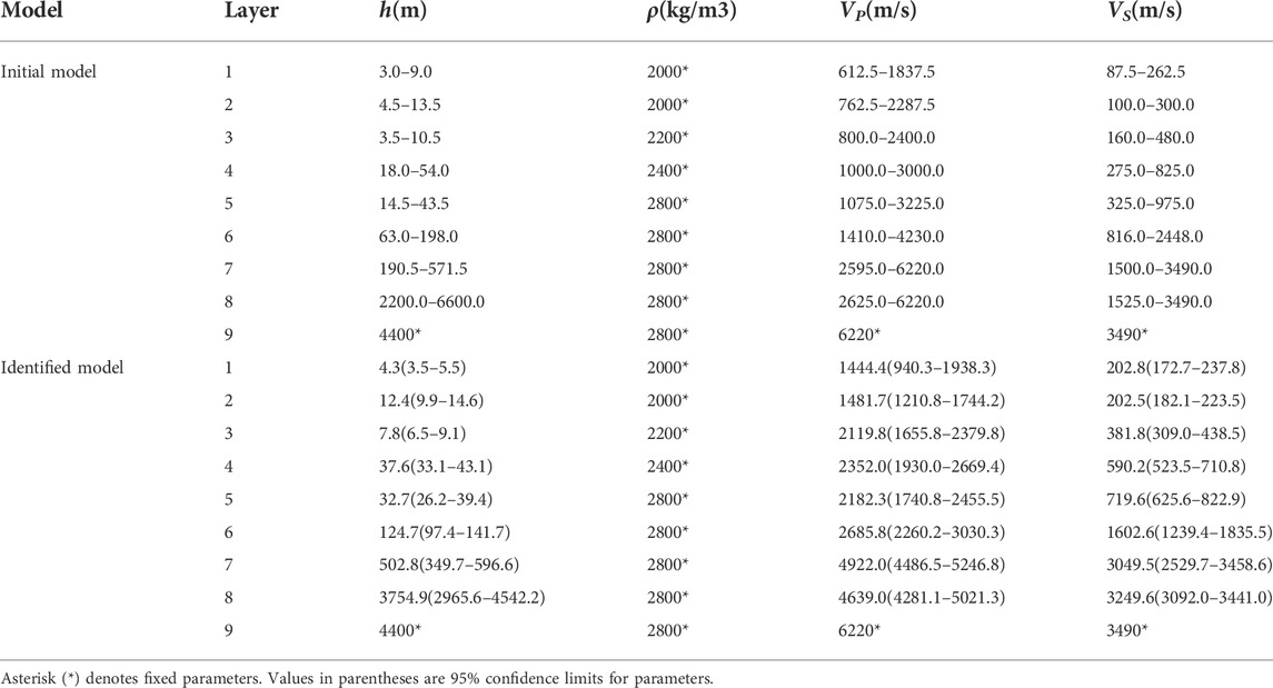
TABLE 3. Verification of joint inversion by the noise-contaminated synthetic case with the GVDA model (see Table 1): initial and identified models.
For the joint inversion of the EHV and DC, the background parameters of inversion were set as follows: the number of generations was 200; the popular size of each generation was 200; the generation gap of the GA was 0.9, the crossover rate was 0.7; the mutation rate was 0.01; and the initial temperature and scale factor (c0) of the SA were 10 °C and 0.99, respectively. The joint inversion process for the minimum objective function ended at the 200th generation, with an inverted structure model as detailed in Table 3. From Figure 6C, we see that the objective function decreases quickly until the number of genetic generations reaches 100, implying that the 200 generations set in the joint inversion are reasonable for this case study. Figure 6D shows that all the iterative models for the Vs. profile, which are colored in terms of generations. We see that these models converge from the searching range to a narrow white area with an increasing number of generations. The corresponding EHV and DC curves of all the possible models colored in terms of values of objective functions are shown in Figures 6E,F; these curves converge to the target curves (the best model) with decreasing objective functions. Figure 7 shows the variability of the inverted parameters (VS, VP, and h) for the second layer along with the objective functions during the convergence. As the objective functions decrease with increasing generation numbers, and the fluctuation range of parameters gradually narrows, and the parameters approach their best values. To estimate the uncertainty associated with the inverted parameters, we calculated the average of the inverted parameters (Avg.), as shown in Table 3. We see that most inverted parameters lie in the range of 95% confidence limits, implying that the best model can be identified for the noise-contaminated EHVs and DCs.
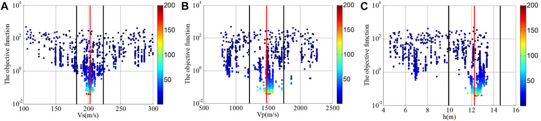
FIGURE 7. Variability of inverted parameters (Vs, Vp, and (H) for the second layer versus objective functions during the converging process, with color bars calibrated in terms of generations. Red and black lines represent the averages and the 95% confidence limits of all the tested parameters. (A) Vs., (B) Vp, (C) h.
To compare with the joint inversion of EHV and DC, the “HV-Inv” program proposed by García-Jerez et al. (2016) and Piña-Flores et al. (2017) was used to conduct a joint inversion of the NHV and DC. The modified SA is adopted as the global optimization method. The inversion parameters were set as follows: the iteration number was 300; the initial population had 200 models; the perturbation range was 10%, and the initial temperature was controlled by the relative misfit increment and probability of acceptance, i.e., 0.1 and 0.5, respectively; the cooling schedule was controlled by the temperature ratio (0.9). From Figure 8A, we see that the objective function reduces quickly with an increase in the number of iterations. Figure 8B shows all the inverted Vs. models. These models converge from the search range to a narrow yellow area with increasing order of appearance of the individuals. Meanwhile, the NHV (Figure 8C) and DC (Figure 8D) also converge to the corresponding target curves. These results show that the HV-Inv is a powerful tool for obtaining subsurface velocity profiles. Because of the vast differences between the two joint inversion methods in terms of their mechanism and inversion algorithms, it is difficult to directly compare them and judge which one is better. However, from the perspective of the inversion result, the best model identified from the joint inversion of the EHV and DC agrees considerably better with the theoretical velocity profile than the best model identified from the joint inversion of the NHV and DC, especially for depths less than 1000 m. Correspondingly, the genetic generations of the joint inversion of the EHV and DC is 200, which is less than the number of iterations for the joint inversion of the NHV and DC, which is 400 in our case.
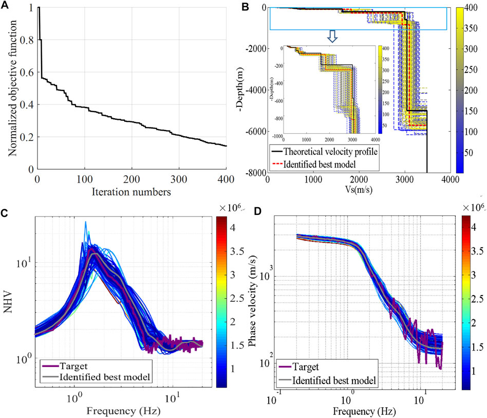
FIGURE 8. The joint inversion of NHV and DC by the noise-contaminated synthetic case with the GVDA model (A) Iterative convergence curve by objective functions versus iteration numbers (B) All the inverted Vs. models, the color bar is calibrated in terms of the order of appearance of the individuals. (C) and (D) The corresponding NHV and DC curves of all the iterative models colored in terms of the value of objective functions which converge to the target curves (purple lines) with decreasing objective functions.
To highlight the advantage of joint inversion, we compared its performance with the one of EHV or DC inversion alone. The EHV and DC inversions follow the same procedure as the joint inversion, except that their objective functions are
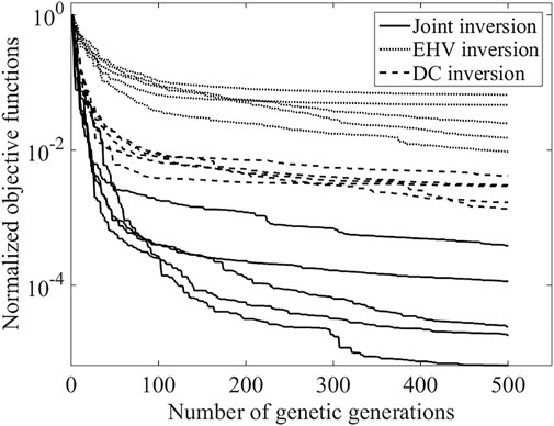
FIGURE 9. Convergence curves with normalized objective functions versus generation numbers by three inversion methods with each for five random numerical experiments.
Figure 10 shows a comparison of these inverted profiles and the corresponding EHV and DC curves obtained by different methods. We see that the joint inversion reproduces the theoretical velocity profile very well (Figure 10A), and the EHV (Figure 10B) and DC (Figure 10C) of the identified best model agree well with the corresponding curves of the theoretical velocity profile. The EHV inversion alone (Figures 10D–F) achieves a good fit to the theoretical EHVs, but the fit for the theoretical DCs is not as good as that for the joint inversion. On the other hand, the DC inversion alone (Figures 10G–I) shows a good fit for the theoretical DCs, but shows a bad fit for the theoretical EHVs.
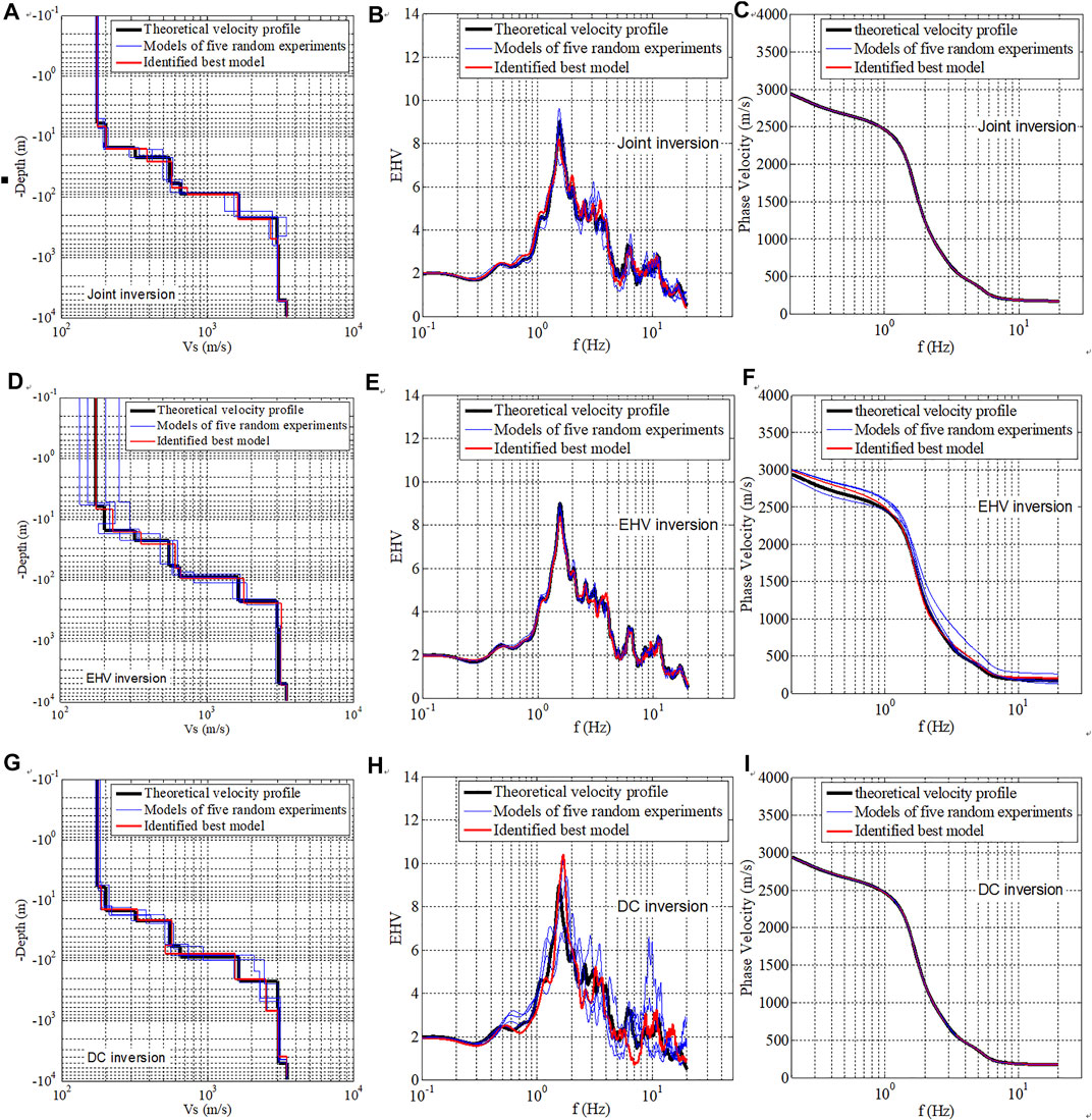
FIGURE 10. Comparison of the theoretical and inverted profiles, EHVs, and DCs by different inversion methods. (A–C) The theoretical and inverted profiles, EHVs, and DCs by proposed joint inversion method. (D–F) The theoretical and inverted profiles, EHVs, and DCs by the EHV inversion alone. (G–I) The theoretical and inverted profiles, EHVs, and DCs by the DC inversion alone. For every inversion methods, five random numerical experiments are conducted.
The proposed joint inversion was applied to observed data from the GVDA site for the P- and S-wave velocities and layer thicknesses. The observed EHV and DC curves were set as target curves, as shown in Figure 11. The observed EHV curve is the average of the EHV curves from several earthquakes. We selected the effective earthquakes that could generate peak ground accelerations greater than 20 cm/s2 and less than 150 cm/s2 in the range of 100 km. As listed in Table 4, 18 events recorded between 1 January 2004, and 31 January 2019, satisfy this requirement. These earthquakes have magnitudes of M2.4–M5.4 with epicentral distances in the range of 4.8–53.4 km. The resulting peak accelerations on the surface of the site range from 57.17 to 146.25 cm/s2. We calculated the EHV curve of each earthquake following the data-processing steps of Rong et al. (2018). There are three processing steps: first, the baseline correction and Chebyshev bandpass filter with a band of 0.1–50 Hz were applied to all the records. Second, a window of more than 5 s, beginning 0.5–1 s before the onset of the S-wave, was taken from each record, and the S-wave onset was visually picked by comparing the horizontal and vertical components for each earthquake. The minimum and maximum S-wave window durations were 5 and 10 s, respectively. Then, the S-wave Fourier spectra were calculated and smoothed by using the Hanning window. Finally, the EHV curve was obtained from the ratio of the geometric mean spectra between the horizontal and vertical components.
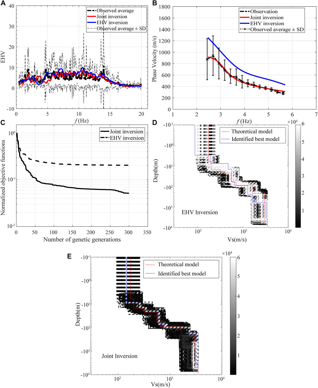
FIGURE 11. (A) Comparison of observed and inverted EHVs by the joint inversion and the EHV inversion alone. The bold black dotted line denotes the observed average EHVs. The thin black dotted lines represent the average ±1 standard deviation (SD) of observations. The red and blue lines denote the best inverted EHVs by the joint inversion and the EHV inversion, respectively. (B) Comparison of observed and inverted DCs. The marked points are measurement points derived from ambient noise array observations. The light error bar represents ±1 SD of observations. The black dotted line is the fitting line of measurement points. The red and blue lines represent the best inverted DCs by the joint inversion and the EHV inversion, respectively. (C) Comparison of convergence curves. (D) Inverted velocity profiles by the EHV inversion alone. (E) Inverted velocity profiles by the joint inversion. In (D) and (E), all the tested models by both the methods are colored in terms of the order of appearance of the individuals. The red and blue lines denote the observed and inverted model profiles, respectively.
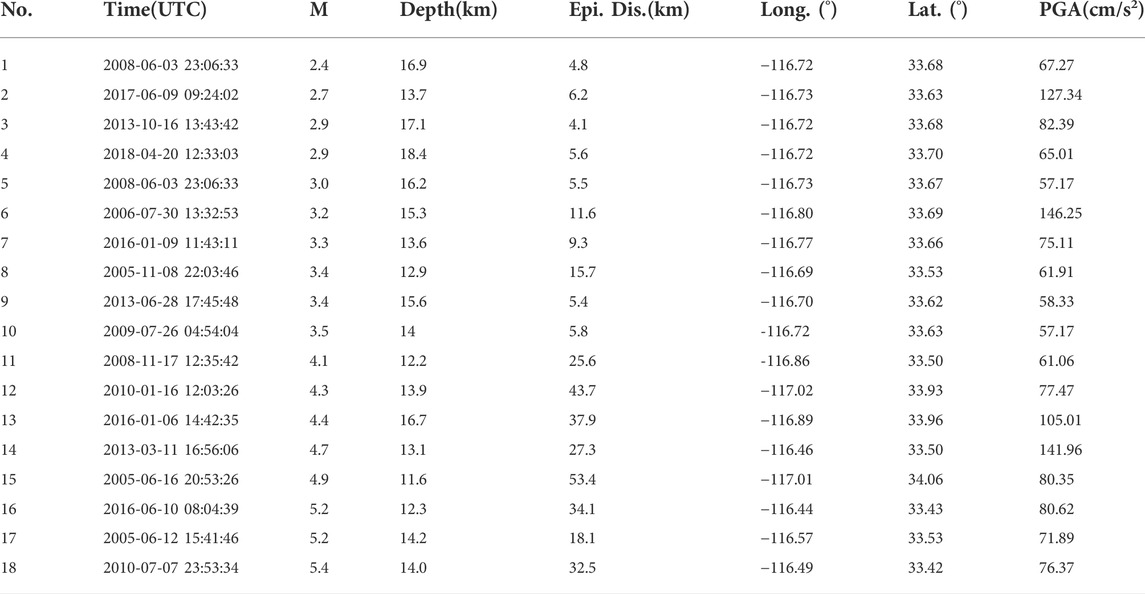
TABLE 4. Earthquake parameters of used accelerograms and corresponding PGAs of vertical array sites.
The observed DC curve is the fitting curve of the phase velocities measured by Liu et al. (2000), as shown in Figure 11B. The measured phase velocities were derived from microtremor recordings by a 10-element nested-triangular array of 100 m aperture on the GVDA site. Although the observed DC curve was only available for about 2–6 Hz, the curve is believed to play an important role in reducing the nonuniqueness in the joint inversion. For comparison, the EHV inversion alone was also conducted following the same procedure and using the relevant parameters. The number of genetic generations for both the inversions was set as 300. The upper and lower limits of velocity and thickness for each layer were in the following ranges (0.5–1.5)VP0 (0.5–1.5)VS0, and (0.5–1.5)h0, with VP0, VS0, and h0 being the P- and S-wave velocities and layer thickness of the measured model, respectively. The other parameters of inversion were set as follows: the popular size of each generation was 200; the generation gap was 0.9; the crossover rate was 0.7; the mutation rate was 0.01; and the initial temperature and scale factor (c0) of the SA were 10°C and 0.99, respectively.
Figure 11 compares the observed and inverted EHVs and DCs for these two inversion methods. We see that the EHV inversion produces a good fit to EHVs but shows obvious discrepancies in the DC curves. The joint inversion produces a good fit for both the EHVs and DCs. Figure 11 compares the convergence curves and inverted velocity profiles obtained by these two inversion methods. We see that the convergence performance (see Figure 11C) of the joint inversion is much better than that of the EHV inversion. The best model identified from the joint inversion in Figure 11E agrees well with the observed model profile with all the tested models colored in terms of generations converging quickly to a narrow white area, and the agreement is much better than in the case of the results (see Figure 11D) obtained by only the EHV inversion. In conclusion, the joint inversion can effectively constrain the model by reducing the non-uniqueness of inversion.
Conventional joint inversions combine the EHV and DC curves with those obtained from array measurements. Such inversions are regarded as the best solution to the non-uniqueness problem arising in the case of the use of EHV or DC inversions alone. To make full use of the additional information of the velocity profile, we proposed an improved joint inversion that combines the Rayleigh wave DCs obtained from array measurements and the EHV obtained from earthquake recordings. We investigated the complementarity of the EHV and surface-wave DCs in the joint inversion through sensitivity analyses. A hybrid global optimization procedure was adopted by combining the GA and SA algorithms. The sensitivity of the inversion parameters was examined to reduce the spatial dimension of inverse problems. We validated the proposed joint inversion by considering a synthetic case of the GVDA model and comparing the results with those obtained by the EHV or DC inversions alone. The proposed method was applied to observation data from the GVDA site for the velocities and thicknesses of soil layers. The main conclusions are summarized as follows:
1. The EHV is more sensitive to sediment thicknesses, especially in the high-frequency range (>10 Hz), and less sensitive to bedrock S-wave velocities. Conversely, the DC is more sensitive to bedrock shear-wave velocities in the low-frequency range (<10 Hz) and less sensitivity to sediment thicknesses. The joint inversion can exploit the complementarity of the EHV and DC to achieve reliable inversion for bedrock shear-wave velocities and sediment thicknesses.
2. The responses of the DC to bedrock S-wave velocities mainly lie in the frequency range less than 2f0, whereas the EHV is sensitive to bedrock S-wave velocities over a wide range of frequencies around f0 and beyond. The frequency complementarity of the EHV and DC can assure the joint inversion for bedrock shear-wave velocities.
3. The sensitivity of inversion parameters demonstrates that the P- and S-wave velocities and thicknesses of soil layers are dominant parameters that affect the EHV or DC responses. It is reasonable to consider VS, VP, and h as the independent variables in the joint inversion.
4. The joint inversion was validated by considering a synthetic case of GVDA site. With increasing generations, the iterative models converged to the measured model rapidly, with most of the inverted model parameters lying in the range of 95% confidence limit. The measured model was identified for the noise-contaminated EHVs and DCs.
5. The joint inversion effectively constrained the model by reducing the non-uniqueness of the inversion. Applications to observed data from the GVDA site achieved perfect convergence of the velocity profiles, with good fits for both the EHVs and DCs. The EHV inversion alone causes obvious discrepancies in the DCs.
All the information of the GVDA, Southern California, used in this study were gathered and authorized by the Earth Research Institute at UCSB. The corresponding observation data can be obtained from http://www.nees.org/(last accessed April 2022). The “gpdc” program used to calculate the theoretical DC can be obtained from http://www.geopsy.org/download.php (last accessed April 2022).
The original contributions presented in the study are included in the article/supplementary material, further inquiries can be directed to the corresponding author.
Conceptualization, MR; methodology, MR; validation, MR and LF; formal analysis, MR and LF; investigation, MR; resources, MR and FS; data curation, MR; writing-original draft preparation, MR, LF and FS; writing-review and editing, LF, FS and WS; visualization, MR and WS; supervision, LF, WS and FS; project administration, MR; funding acquisition, MR and FS. All authors have read and agreed to the published version of the manuscript.
This study is supported by the Natural Science Foundation of China (Grants No. 41720104006 and 51878625) and by DGAPA-UNAM under (Project IN107720).
The authors wish to thank S. Parolai who offered references and helped in the joint inversion method. The authors also appreciate J.E. Plata and G. Sánchez and their team of the Unidad de Servicios de Información (USI) of the Institute of Engineering-UNAM for locating useful references.
The authors declare that the research was conducted in the absence of any commercial or financial relationships that could be construed as a potential conflict of interest.
All claims expressed in this article are solely those of the authors and do not necessarily represent those of their affiliated organizations, or those of the publisher, the editors and the reviewers. Any product that may be evaluated in this article, or claim that may be made by its manufacturer, is not guaranteed or endorsed by the publisher.
Aki, K. (1957). Space and time spectra of stationary stochastic waves with special reference to microtremors. Bull. Earthq. Res. Inst. 35, 415
Arai, H., and Tokimatsu, K. (2004). S-wave velocity profiling by inversion of microtremor H/V spectrum. Bull. Seismol. Soc. Am. 94 (1), 53–63. doi:10.1785/0120030028
Bignardi, S., Mantovani, A., and Abu Zeid, N. (2016). OpenHVSR: Imaging the subsurface 2D/3D elastic properties through multiple HVSR modeling and inversion. Comput. Geosci. 93, 103–113. doi:10.1016/j.cageo.2016.05.009
Bonilla, L. F., Steidl, J. H., Gariel, J. C., and Archuleta, R. J. (2002). Borehole response studies at the garner valley downhole array, southern California. Bull. Seismol. Soc. Am. 92 (8), 3165–3179. doi:10.1785/0120010235
Cui, J. W. (2004). An improved global optimization method and its application to the inversion of surface wave dispersion curves. Chin. J. Geophys. 47 (3), 521.
Fäh, D., Kind, F., and Giardini, D. (2001). A theoretical investigation of average H/V ratios. Geophys. J. Int. 145 (2), 535–549. doi:10.1046/j.0956-540x.2001.01406.x
García-Jerez, A., Piña-Flores, J., Sánchez-Sesma, F. J., Luzón, F., and Perton, M. (2016). A computer code for forward calculation and inversion of the H/V spectral ratio under the diffuse field assumption. Comput. Geosciences 97, 67–78. doi:10.1016/j.cageo.2016.06.016
Gibbs, J. F. (1989). Near-surface P- and S- wave velocities from borehole measurements near Lake Hemet, California. U.S. Geol. Surv. Open File rept. 89, 630.
Gouedard, P., Cornou, C., and Roux, P. (2008). Phase-velocity dispersion curves and small scale geophysics using noise correlation slantstack technique. Geophys. J. Int. 172 (3), 971–981. doi:10.1111/j.1365-246x.2007.03654.x
Herak, M. (2008). Model HVSR-A Matlab tool to model horizontal-to-vertical spectral ratio of ambient noise. Comput. Geosci. 34, 1514–1526. doi:10.1016/j.cageo.2007.07.009
Kawase, H., Mori, Y., and Nagashima, F. (2018). Difference of horizontal-to-vertical spectral ratios of observed earthquakes and microtremors and its application to S-wave velocity inversion based on the diffuse field concept. Earth Planets Space 70 (1), 1. doi:10.1186/s40623-017-0766-4
Kawase, H., Sánchez-Sesma, F. J., and Matsushima, S. (2011). The optimal use of Horizontal-to-Vertical spectral ratios of earthquake motions for velocity inversions based on diffuse field theory for plane waves. Bull. Seismol. Soc. Am. 101 (5), 2001–2014. doi:10.1785/0120100263
Lawrence, J. F., and Wiens, D. A. (2004). Combined receiver-function and surface wave phase-velocity inversion using a niching genetic algorithm: application to patagonia. Bull. Seismol. Soc. Am. 94 (3), 977–987. doi:10.1785/0120030172
Liu, H. P., Boore, D. M., Joyner, W. B., Oppenheimer, D. H., Warrick, R. E., Zhang, W. B., et al. (2000). Comparison of phase velocities from array measurements of Rayleigh waves associated with microtremor and results calculated from borehole shear-wave velocity profiles. Bull. Seismol. Soc. Am. 90 (3), 666–678. doi:10.1785/0119980186
Louie, J. N. (2001). Faster, better: Shear-wave velocity to 100 meters depth from refraction microtremor arrays. Bull. Seismol. Soc. Am. 91 (2), 347–364. doi:10.1785/0120000098
Mosegaard, K., and Sambridge, M. (2002). Monte Carlo analysis of inverse problems. Inverse Probl. 18, 29–54. doi:10.1088/0266-5611/18/3/201
Nagashima, F., Matsushima, S., Kawase, H., Sanchez-Sesma, F. J., Hyakawa, T., Satoh, T., et al. (2014). Application of horizontal-to-vertical spectral ratios of earthquake ground motions to identify subsurface structures at and around the K-net site in tohoku, Japan. Bull. Seismol. Soc. Am. 104 (5), 2288–2302. doi:10.1785/0120130219
Nakamura, Y. (1989). A method for dynamic characteristics estimation of subsurface using microtremor on ground surface. QR Railw. Tech. Res. Inst. 30 (1), 25
Parolai, S., Picozzi, M., Richwalski, S. M., and Milkereit, C. (2005). Joint inversion of phase velocity dispersion and H/V ratio curves from seismic noise recordings using a genetic algorithm, considering higher modes. Geophys. Res. Lett. 32, L01303. doi:10.1029/2004gl021115
Pecker, A., and Mohammadioum, B. (1993). “Garner Valley: analyse statistique de 218 enregistrements seismiques,” in Proceeings of the 3eme colloque national AFPS. France: Saint-Remy-les-Chevreuse, Paris.
Picozzi, M., and Albarello, D. (2007). Combining genetic and linearized algorithms for a two-step joint inversion of Rayleigh wave dispersion andH/Vspectral ratio curves. Geophys. J. Int. 169, 189–200. doi:10.1111/j.1365-246x.2006.03282.x
Picozzi, M., Parolai, S., and Richwalski, S. M. (2005). Joint inversion of H/V ratios and dispersion curves from seismic noise: estimating the S-wave velocity of bedrock. Geophys. Res. Lett. 32 (11), L11308. doi:10.1029/2005gl022878
Pina-Flores, J., Perton, M., Garcia-Jerez, A., Carmona, E., Luzon, F., Molina-Villegas, J. C., et al. (2017). The inversion of spectral ratio H/V in a layered system using the diffuse field assumption (DFA). Geophys. J. Int. 208 (1), 577–588.
Rong, M. S., Fu, L. Y., and Li, X. J. (2018). Inversion of site velocity structure using a hybrid optimization algorithm based on HVSRs of accelerograms recorded by a single station. Chin. J. Geophys. 61 (3), 938. doi:10.6038/cjg2018L0171
Sánchez-Sesma, F. J., Rodriguez, M., Iturraran-Viveros, U., Luzon, F., Campillo, M., Margerin, L., et al. (2011). A theory for microtremor H/V spectral ratio: application for a layered medium. Geophys. J. Int. 186 (1), 221–225. doi:10.1111/j.1365-246x.2011.05064.x
Santos, A. B., Sampaio, E. E. S., and Porsani, M. J. (2005). A robust two-step inversion of complex magnetotelluric apparent resistivity data. Stud. Geophys. Geod. 49 (1), 109–125. doi:10.1007/s11200-005-1628-2
Scherbaum, F., Hinzen, K. G., Ohrnberger, M., Ohrnberger, M., and Herrmann, R. B. (2003). Determination of shallow shear wave velocity profiles in the Cologne, Germany area using ambient vibrations. Geophys. J. Int. 152 (3), 597–612. doi:10.1046/j.1365-246x.2003.01856.x
Tada, T., Cho, I., and Shinozaki, Y. (2009). New circular-array microtremor techniques to infer love-wave phase velocities. Bull. Seismol. Soc. Am. 99 (5), 2912–2926. doi:10.1785/0120090014
Theodulidis, N., Bard, P. Y., Archuleta, R., and Bouchon, M. (1996). Horizontal-to-vertical spectral ratio and geological conditions: the case of Garner valley downhole array in southern california. Bull. Seismol. Soc. Am. 86 (2), 306–319. doi:10.1785/bssa0860020306
Wathelet, M. (2005). Array recordings of ambient vibrations: surface-wave inversion. Liège: University of Liège. [dissertation/doctor’s thesis]. [Belgium].
Wathelet, M., Chatelain, J., Cornou, C., Giulio, G. D., Guillier, B., Ohrnberger, M., et al. (2020). Geopsy: a user-friendly open-source tool set for ambient vibration processing. Seismol. Res. Lett. 91 (3), 1878–1889. doi:10.1785/0220190360
Wu, H., Masaki, K., Irikura, K., and Sánchez-Sesma, F. J. (2017). Application of a simplified calculation for full-wave microtremor H/V spectral ratio based on the diffuse field approximation to identify underground velocity structures. Earth Planets Space 69, 162. doi:10.1186/s40623-017-0746-8
Keywords: earthquake-based HVSR (EHV), joint inversion, site velocity structures, Garner valley site, dispersion curve (DC)
Citation: Mianshui R, Li-Yun F, Francisco José S-S and Weijia S (2022) Joint inversion of earthquake-based horizontal-to-vertical spectral ratio and phase velocity dispersion: Applications to Garner Valley. Front. Earth Sci. 10:948697. doi: 10.3389/feart.2022.948697
Received: 20 May 2022; Accepted: 13 July 2022;
Published: 08 August 2022.
Edited by:
Yefei Ren, Institute of Engineering Mechanics, China Earthquake Administration, ChinaReviewed by:
Dun Wang, China University of Geosciences Wuhan, ChinaCopyright © 2022 Mianshui, Li-Yun, Francisco José and Weijia. This is an open-access article distributed under the terms of the Creative Commons Attribution License (CC BY). The use, distribution or reproduction in other forums is permitted, provided the original author(s) and the copyright owner(s) are credited and that the original publication in this journal is cited, in accordance with accepted academic practice. No use, distribution or reproduction is permitted which does not comply with these terms.
*Correspondence: Fu Li-Yun, bGZ1QHVwYy5lZHUuY24=
Disclaimer: All claims expressed in this article are solely those of the authors and do not necessarily represent those of their affiliated organizations, or those of the publisher, the editors and the reviewers. Any product that may be evaluated in this article or claim that may be made by its manufacturer is not guaranteed or endorsed by the publisher.
Research integrity at Frontiers
Learn more about the work of our research integrity team to safeguard the quality of each article we publish.