 Daniela Famiani
 Fabrizio Cara1
 Giuseppe Di Giulio
 Maurizio Vassallo
95% of researchers rate our articles as excellent or good
Learn more about the work of our research integrity team to safeguard the quality of each article we publish.
Find out more
ORIGINAL RESEARCH article
Front. Earth Sci. , 19 August 2022
Sec. Geohazards and Georisks
Volume 10 - 2022 | https://doi.org/10.3389/feart.2022.937848
This article is part of the Research Topic New Challenges for Seismic Risk Mitigation in Urban Areas View all 11 articles
The presence of normal fault systems in central Italy, outcropping or hidden below Quaternary covers in intra-mountain basins, is the expression of the Neogene–Quaternary evolution of the area, characterized by an extensional tectonic regime following the fold and thrust structuring of the Apennine orogen. Italian urban settlements of central Italy are developed on hills or mountains but also in lowland areas, which are often set up in sedimentary basins. In this framework, urban centers found close to fault lines are common, with strong implications on the seismic risk of the area. In this work, we performed a dense seismological passive survey (88 single-station ambient noise measurements) and used the horizontal-to-vertical spectral ratio (HVNSR) technique to investigate hidden faults in the Trasacco municipality located in the southern part of the Fucino Basin (central Italy), where microzonation studies pointed out hypothetical fault lines crossing the urban area with the Apennine orientation. These hidden structures were only suggested by previous studies based on commercial seismic lines and aerial photogrammetry; their presence in the basin area is confirmed by our measurements. This case study shows the potentiality of using the HVNSR technique in fault areas to have a preliminary indication of anomalous behaviors, to be investigated later with specific geophysical techniques. Our approach can support microzonation studies whenever fault zones are involved, especially in urban areas or in places designated for future developments.
Seismic microzonation studies are often carried out at a basic level, sometimes leaving open scientific points that require further ad hoc investigations to be solved. In this study, we face one of these cases regarding the Fucino Basin (hereinafter FB), a large intra-mountain continental basin in central Italy. The FB was the greatest lake of central Italy until its complete drainage at the end of the 19th century and has a tectonic origin related to the presence of important normal fault systems. Here, we focus on the southern part of the FB, specifically close to Trasacco village (red square in Figure 1). In 2013, the Trasacco municipality (about 6,000 inhabitants) has been the object of a seismic microzonation study, and one of the main objectives was to clarify the position of the Trasacco fault, an active and capable NW-SE oriented normal structure following the elongation of the Vallelonga valley (see zoom in Figure 1 for the location). In fact, the issue of characterizing and zoning active and capable faults is crucial for urban planning purposes and also for ensuring safe conditions to the pre-existing buildings. Despite the large amounts of data (geognostic, geophysical, and geotechnical) collected by professional geologists during the microzonation activities, no evidence of the fault was found in the urbanized area. The spatial continuation of this fault in the northern direction of the basin area is also uncertain.
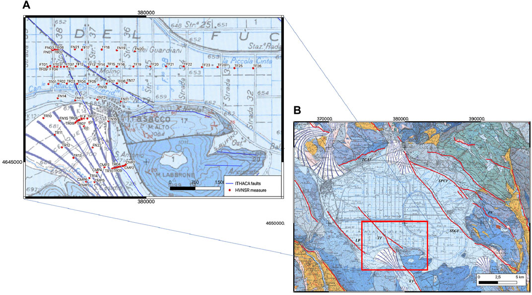
FIGURE 1. Geological map of the Fucino Basin (from Ghisetti and Vezzani, 1998) with the schema of the main fault lines in red (B). Zoom of the study area with red dots representing the HVNSR investigations and fault lines in blue from the ITHACA database (A).
Hence, we decided to perform a geophysical study devoted to identifying the extension of the Trasacco fault in the basin area and other possible tectonic structures in it. In particular, we performed a wide campaign of single-station ambient noise recordings, using the well-known horizontal-to-vertical spectral ratio (HVNSR) technique as the method of analysis (Nakamura, 1989). Some of these data, which were recorded simultaneously at different locations, have been also used to roughly estimate the shear-wave velocities of the sedimentary layers. The HVNSR results are discussed under two different perspectives: first, we adopt a classical interpretation scheme to get a first-order reconstruction of the subsoil of the study area through the identification of the fundamental resonance frequency (f0) of the investigated sites; and second, we perform a directional analysis on HVNSR, for e.g., by rotating the horizontal components of the ground motion for sites close to tectonic elements. The purpose of this latter study was to identify a sort of signature related to specific complexities of the investigated sites and possibly linked to the presence of the Trasacco fault and all the other tectonic structures. The correlation between these observations and the geology is supported by the availability of other relevant previous studies in the Fucino Basin.
The FB is an intra-mountain lacustrine basin with a tectonic origin. Some of the faults that originated in the basin are able to generate large seismic events, such as the 13 January 1915 M 7.0 Avezzano earthquake, which completely destroyed the town of Avezzano and caused about 30,000 casualties. The FB is infilled by Upper Pliocene–Holocene lacustrine and alluvial deposits (Bard and Bouchon, 1980a; Bard and Bouchon, 1980b; Giraudi, 1988; Bosi et al., 1995), which unconformably overlie Meso-Cenozoic carbonate and Neogene terrigenous successions (Cavinato et al., 2002). Quaternary deposits also include alluvial fans made by the dismantling of the surrounding reliefs. FB is the largest intra-mountain endoreic depression of the Apennines, filled by a well-preserved thick Quaternary continental succession (Mannella et al., 2019), representing an important record to reconstruct the geological evolution of central Italy (volcanic eruptions and climate changes). According to Galadini et al. (1995) and Cavinato et al. (2002), from a neo-tectonic point of view, the evolution of the FB has been mainly affected by the activity of two systems of faults that border the northern and eastern sectors of the area. These two can be described as the “active” sides of the basin, and they can be easily distinguished, for the evidence of structural elements and outcropping geological units, from the southern and western parts of the basin which, conversely, are supposed to have a passive role in the genesis of the plain.
The total subsidence of the area may be defined as the sum of the hanging-wall subsidence generated by the normal fault and sediment compaction, and the regional subsidence or uplift (Doglioni et al., 1998).
From the analysis of surface geological data and the interpretation of seismic lines, Cavinato et al. (2002) divided the sedimentary infilling of FB in two different groups of stratigraphic units: Lower and Upper Units. The Lower Units (Upper Pliocene) crop out in the northern and north-eastern margins of the basin and consist of breccia, fluvial, and marginal to open-lacustrine deposits. The Upper Units (Lower Pleistocene–Holocene) are represented by marginal lacustrine/fluvial deposits; thick coarse-grained fan-delta deposits are inter-fingered with fluvial–lacustrine deposits at the foot of the main relief. It is worth mentioning that some of the articles published for the area aimed at studying the characteristics of the recent units more in detail: general descriptions of continental deposits (Zarlenga, 1987), more specific analysis of morphotectonic (Bard and Bouchon, 1985; Blumetti et al., 1993) or geomorphological features, as alluvial fans (Frezzotti and Giraudi, 1992) or terraces (Accordi 1975; Messina 1996).
Focusing more on the structural elements present in FB, the main faults are (right side in Figure 1): the Tremonti–Celano–Aielli Fault (TCAF) (WSW–ENE) and S. Potito–Celano Faults (NW-SE) in the north; the Luco Fault (LF) in the west; and the Trasacco Fault (TF) and Villavallelonga Fault (VF), the Pescina–Celano Fault (PCF), and the Serrone Fault (NW–SE) in the southern and southeastern parts of the basin. Recently, Lanari et al. (2021) proposed a structural analysis of the FB making inferences on how sediment loading/unloading influences the dynamics of fault systems, demonstrating positive feedback between sedimentation and faulting.
An important contribution for reconstructing the FB and understanding the role played by every structural element in its general evolution is given by the interpretation of industrial seismic reflection profiles [location by Patruno and Scisciani, (2021) displayed in Figure 2] which can identify the subsurface geometry of outcropping faults and also image the subsoil layers and their thickness.
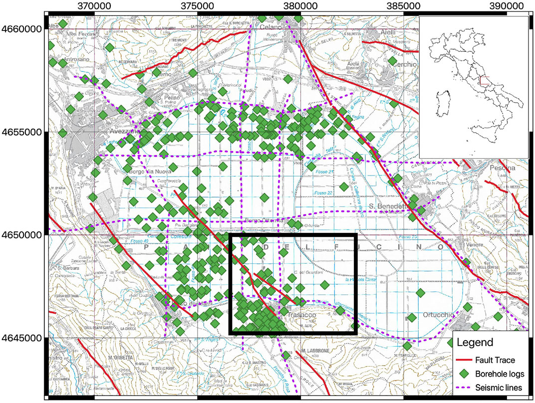
FIGURE 2. Map of previous investigations: the fault lines from the ITHACA database are in red, and boreholes from ISPRA and Ente Fucino are in green. The study area is delimited by a black box.
For some authors, most of the thickness of the fluvio-lacustrine succession (more than 800 m) (Cavinato et al., 2002; Patacca et al., 2008; Cara et al., 2011) is generated by the San Benedetto–Serrone–Gioia dei Marsi fault (hereinafter SSGF) system, located in the eastern margin of the FB. Some others (Patruno and Scisciani 2021), conversely, acknowledged the maximum thickness of the Quaternary deposits (∼1,750 m) in two depocentral areas, for the combined activity of the TCAF and San Benedetto–Serrone–Gioia dei Marsi Fault (SSGF).
In addition to the contribution of seismic lines, some authors (Cella et al., 2021; Mancinelli et al., 2021) recently performed studies on the magnetic anomalies of the FB. Cella et al. (2021) not only carried out a 3D gravity model for evaluating the depth of the Meso-Cenozoic carbonate bedrock but also provided additional constraints on the position of the known hidden faults. Both the aforementioned research works discuss the paleogeographic and paleotectonic evolutions of the FB confirming the presence of a major depocenter as the effect of the activity of the SSGF in the eastern part of the FB, and a second depocenter whose evolution is ascribable to the activity of the Trasacco fault, on its western side.
Mancinelli et al. (2021) reconstructed 2D gravity models along a grid of seven sections crossing the basin, in which is shown the influence of the Miocene flysch deposits in the observed residual general anomaly present in the FB. They also highlighted the thickness of Miocene deposits, as modeled in the sections. A higher thickness of flysch deposits (around 1,100 m) is found in the western part of the basin, consistent with a syn-orogenic emplacement of the deposits, and decreases toward the south and east.
Concerning the shallower part of the subsoil, paleo-seismological studies in FB started during the ‘80s (Giraudi 1986; Serva et al., 1986; Giraudi 1988; Galadini and Galli 1996; Michetti et al., 1996; Galadini et al., 1997; Galadini et al., 1997), and a collection of all the results is summarized in Galadini and Galli (1999). Amoroso et al. (2016) also presented a synoptic review of all the paleoseismic data collected for the FB, including information related to the slip rates of all the tectonic structures, deriving a possible overall extension rate across the basin of about 3–3.5 mm/yr.
The study area of this work is located in the Trasacco municipality, going from the urban area toward the central part of the basin. The target area is interesting due to the presence of alluvial fans in the urbanized area and of buried faults in the most rural area. Although there is no evidence of fault scarps in this area, aerial photos show a straight NW-SE-oriented lineament (Oddone 1915; Galadini and Galli 1999) which represents the contact between soils with different lithologies. This feature addressed the excavation of a huge number of hand boreholes to precisely locate the fault in the field. Paleo-seismological trenches were performed in the area by Galli et al. (2012); Galadini and Galli, (1996), together with many boreholes and trenches, studied the Trasacco fault and reconstructed the vertical displacement along its length and associated them to specific historical seismic events. Results of their study highlighted the multiple activation of this fault during the Holocene: the most recent event is related to the 1915 Fucino earthquake and the previous one is dated to fifth–sixth A.D. The slip rate of the fault obtained from available data decreases toward its NW edge, reflecting the trend of its offsets toward the center of the basin.
The single-station noise measurements were performed by using two different seismic stations: the Reftek-130 and Lennartz MarsLite digitizers modified by SARA electronic instruments connected to Lennartz 3D/5s velocimetric sensors and Terrabot (SARA electronic instruments) units, and all-in-one 24-bit digitizers with internal 4.5 Hz sensors. For all the stations, time synchronization was ensured by GPS antennas.
Overall, the survey consisted of 88 noise measurements performed in different time periods (zoom in Figure 2), of which 12 have been visually inspected to evaluate the quality of data, by the analysis of the Fourier spectra. For some sites with bad quality data, we have repeated the measurement in different time periods (eg., TB** and FN** measures located along Section 1 in Figure 3, zoomed location in Figure 11). The minimum length of recording was fixed at 90 min, in order to allow a good statistic of the results in the frequency domain of interest. The sampling rate was set to 200 or 250 sps. Some sets of measurements were collected simultaneously.
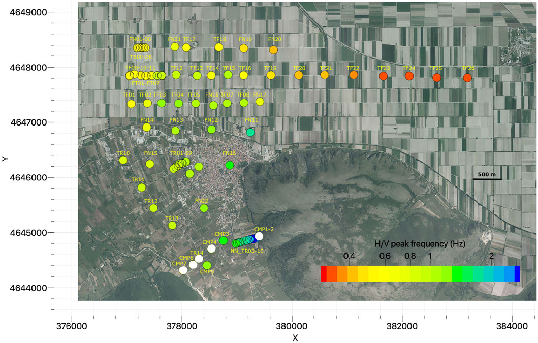
FIGURE 3. F0 map with the location of the HVNSR measurements (results in Supplementary Appendix S1). The color band represents the f0 value of each point of measure. White circles represent measures with no resonance peak or with bad quality data.
The positions of the measurement points were chosen with the aim to obliquely cross the hypothetical surface projection of the Trasacco faults (Apennine trend of the tectonic structures), as evidenced from the seismic lines’ interpretation.
Overall, the final geometry of the survey can be seen as a set of transects trying to cross orthogonally to the supposed fault line. Actually, the survey covered the entire study area but with an irregular density and with special attention to the basin area in the north of Trasacco where buried fault structures were suggested by previous studies. In fact, whenever a set of measurements ended, the following measurements were performed trying to refine the previous results. For this reason, the distance between stations of each transect was largely variable, ranging from 30 to 500 m.
One of the transects (corresponding to Section 2 in Figure 3) is 6 km long and largely exceeds the Trasacco area. The aim of this measurement line was to investigate and understand the general trend of the main impedance contrasts in the FB at a wider scale.
Single-station noise data were analyzed using Geopsy software (Wathelet et al., 2020) in terms of HVNSR curves (Nakamura, 1989). The analysis was also computed by rotating the horizontal components from 0 to 180° in steps of 10. The complete steps of analysis, developed within the SESAME project (Site Effects Using Ambient Excitations, SESAME 2004), consist of:
1) Applying an anti-trigger algorithm that selects 40s-long windows into the whole three-component recordings, in order to avoid short or anomalous transients often of anthropic origins. The chosen length of the windows, 40s, guaranteed a good frequency sampling according to the targets of the study;
2) removing mean and linear trends from each time window;
3) tapering the edges of the time windows;
4) rotating the horizontal components of the desired angle;
5) computing the Fourier spectra of the three components;
6) smoothing the Fourier spectra using the logarithmic Konno–Ohmachi algorithm (Konno and Ohmachi, 1998), with the bandwidth coefficient b equal to 40;
7) by visual inspection, identifying regular trends on the Fourier spectra and discarding windows affected by possible anthropic disturbances;
8) dividing the rotated horizontal spectra by the vertical spectrum for the selected windows;
9) geometrically averaging the spectra or the HVNSR obtained for each 40s-long window.
The classical computation of HVNSR does not imply the directional analysis. In this case, the two horizontal components are NS (0°) and EW (90°), and after points e) and f), the two horizontal spectra are simply merged using an arithmetic mean, in order to have a unique horizontal spectrum for each 40s-long window.
Results of the directional analysis of HVNSR are often shown in an image map, with frequency as x-axis, angle of rotation as y-axis, and the color of the map that is representative of the amplitude of HVNSR for each frequency/angle pair. Nevertheless, the same results can also be shown by plotting the rotated HVNSR curves all together. This kind of representation is useful to prove any possible anisotropy of the wavefield. The classical post-processing of HVNSR (considering only the merged NS and EW components) consists of looking at the shape of each curve and retrieving the main peak, also called the fundamental or resonance frequency (f0) of the selected site. This step is not always trivial. Sometimes, the peak is unique, very narrow, and with an amplitude greater than 2. Therefore, the resonance peak can be recognized easily. On the contrary, there are several peaks very often, or the main peak is very broad and/or weak. In these cases, the user experience on the interpretation of the results is really crucial because it requires a general overview of both the geological setting and the HVNSR curves on the surrounding area of the selected measurement point. Hence, we were able to associate a resonance frequency value for all stations, except for some flat HVNSR curves (Supplementary Appendix S1). The frequency peaks are selected between 0.2 and 4 Hz, discarding higher frequency values because they were considered irrelevant for the scope of this work.
A way of representing the results obtained by the HVNSR technique is to plot the resonance frequencies in a map (Figure 3) and interpolate them (Figure 4) to produce a contour plot (ISPRA, 1881; ITHACA Working Group, 2019; Mascandola et al., 2019). An inverse distance weighting (IDW) method, for e.g., a deterministic spatial interpolation model, was applied to interpolate f0 data in the map. The general premise of this method is that the attribute values of any given pair of points are related to each other, but their similarity is inversely proportional to the distance between the two locations (Lu and Wong, 2008).
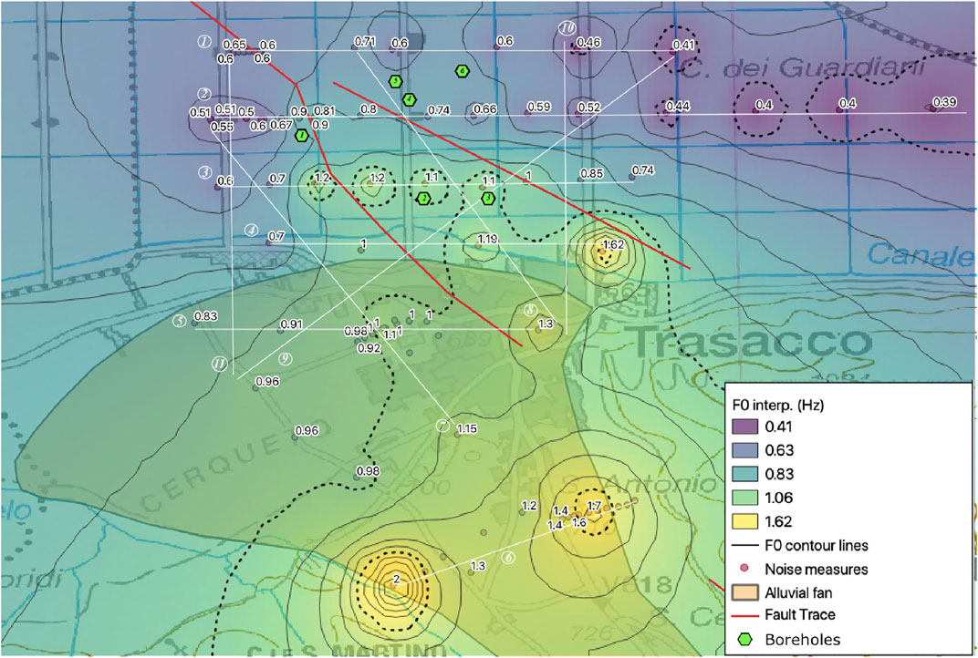
FIGURE 4. Map of f0 interpolation. Red dots represent the noise measurements with the f0 value reported. The fault lines in red come from the ITHACA database. Green diamonds represent the boreholes considered for 1D modeling (Figure 8).
Another way of visualizing information from HVNSR results is to consider the entire curves, not the resonance frequency alone. For each transect, we produced an image map interpolating the HVNSR curves along the distance (Figures 5, 6). The linear regression method was applied to data to find the best fitting line to plot, and then spatial coordinates (in meters) were projected on it. This kind of plot is helpful to imagine subsoil heterogeneities (Joyner et al., 1981; Famiani et al., 2020): the amplitude of spectral ratio curves is represented in a colored scale, while the XY axis shows the distance of the single noise measurement with respect to the beginning of the transect and the frequency values of HVNSR, respectively.
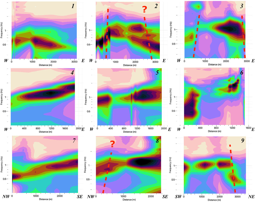
FIGURE 5. HVNSR contour plots of investigations organized along the transects. The plots correspond to sections 1–9 (see location in Figure 4).
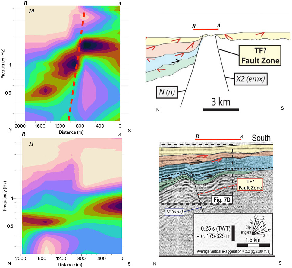
FIGURE 6. HVNSR contour plots of Section 10 and Section 11 located along seismic line 4 (top) and line 2 (bottom) interpreted in Patruno and Scisciani, (2021). The correspondence between the location of HVNSR contour-plot sections and the seismic line is reported with a red line and A and B extremes of the sections. A sketch of the hypothetical fault is also reported with a dotted red line.
Many of the noise measurements were collected in synchronous acquisition. Hence, the simultaneous recordings acted as a passive array of seismic stations, located in 1D (lines along transects) or 2D (when positioned in grids or irregular geometries) configurations. These kinds of data can then be used to retrieve the dispersion characteristics of the noise wavefield crossing the stations and finally estimating a velocity profile for the shallower layers of the area. Unfortunately, among all the possible simultaneous sets of stations, only the ones including stations from TB00 to TB08 (western part of Section 1 in Figure 11) gave reliable results.
To compute the dispersion curve from the noise data, we first calculated the cross-correlation (CC) functions between the vertical components of station pairs. The synchronized recordings of vertical components were first processed using the one-bit normalization and the spectral whitening (Bensen et al., 2007). Then, the CC functions were computed for each station pair. To compute the dispersion curve of the seismic signals emerging from the CC functions, we applied a velocity analysis to them. The method is similar to the constant velocity stack (CVS) analysis (Yilmaz, 1987; Yamanaka et al., 1994), which is very popular in active seismic reflection processing and has already been used on CC results for different Italian areas (Vassallo et al., 2019; Di Giulio et al., 2020). The CC functions were filtered in different frequency bands starting from 0.5 to 20 Hz. For each frequency band, the CC functions were shifted back in time according to the theoretical surface travel times computed for different constant velocities starting from 50 m/s until 900 m/s using a velocity step of 10 m/s. Then, the phase-weighted Stack (PWS, Schimmel and Paulssen, 1997) was computed, and the absolute maximum of the PWS stack was used to estimate the presence of a horizontally aligned phase in the corrected seismic section. For each filter, the maximum stack function provides the velocity of the surface waves at the considered frequency.
The dispersion curves obtained through CC functions and the velocity analysis were finally inverted in order to obtain a preliminary 1D velocity profile of the subsoil. To improve the inversion process, the HVNSR results have also been used as constraints. In particular, the inversion process has been imposed to fit as best as possible to the part of the HVNSR curve around the resonance peak. The computation of the velocity models has been performed using Geopsy software, in particular, the dinver tool (Wathelet 2008): this code adopts a Monte Carlo-like approach, the so-called neighborhood algorithm, to search for subsoil velocity models that fit the data.
The initial parameterization of the subsoil consisted in a four-layered model over a half-space for all the tested sites, for which the shallower layer is assumed to have a linear increasing Vs. However, in order to avoid strict constraints to the process, a wide variability of the parameterization in terms of thickness and Vs of the layers was allowed.
The average spectral ratio curves of all the sites are plotted in Supplementary Appendix S1.
It is worth noting that most of the HVNSR curves showing a single peak, multiple peaks, or flat shapes (CMP2, CMP4, and CMP5) occur in the frequency range of interest (0.2—4 Hz). This observation suggests the presence of a unique strong impedance contrast in the subsoil, likely ascribable to the geological interface between the lacustrine filling and the bedrock of the area (Meso-Cenozoic carbonate and Neogene terrigenous successions). For the stations installed in correspondence to the deeper part of the basin (TF18, FN19, and FN20 in Section 1 and Figure 11 and from TF19 to TF26 in Section 2 and Figure 12), a second broad amplification peak after the fundamental one occurs.
Figures 3, 4 show the resonance frequency and the f0 value interpolation maps, respectively. The distribution of f0 follows a double trend: in the northern part of the maps (Sections 1, 2, and 3, location in Figure 4), there is a decrease of f0 moving toward north, whereas in the southern part (Sections 4, 5, and 6, location in Figure 4) the f0 values decrease toward NW. Contour plots of HVNSR curves along the sections are reported in Figure 5.
Sections from 1 to 6 are all W-E oriented and display HVNSR amplitude contouring from north to south of the study area. Assuming that the depth of the impedance contrast is linearly proportional to 1/f0, we can find a reasonable geologic interpretation of f0. Hence, we can state that sections 1, 2, and 3, representative of the basin part of the Trasacco municipal territory, show a regular decrease in f0, which means the deepening of the impedance contrast toward north and, at the same time, a trend that resembles a structural high feature in the central parts, especially in sections 2 and 3. Moving from the eastern part of Section 2, some HVNSR measurements were performed to follow the general E-W trend of the basin toward the eastern depocenter of the FB (Section 2b—Figure 7). A second broad resonance peak is displayed for the eastern part of this section, which could suggest the presence of a shallower impedance contrast unreachable by all the boreholes available in the area.
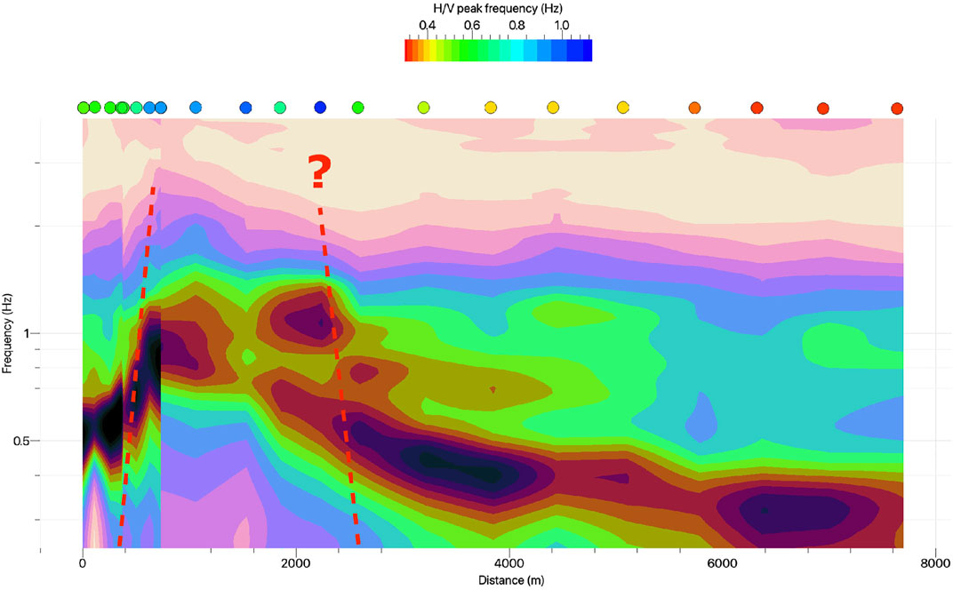
FIGURE 7. HVNSR section plot of Section 2b. The colored circles indicate the position of each ambient noise measurement along the section and their f0 value. A sketch of the hypothetical fault is reported with a dotted red line.
Section 4 represents a transition zone where there is a change in the f0 trend compared to sections 1, 2, and 3. In fact, it shows a more flat and continuous shape of the impedance contrast without any evidence of the structural high.
Sections 5–6 cross the alluvial fan, and the interpretation of the contouring of HVNSR is less straightforward because there is no information about the total thickness and shear-wave velocity of the alluvial fan deposits. When Section 5 shows, similar to Section 4, a continuous seismic interface, Section 6 reveals a typical valley shape, except for the low-frequency amplification for stations CMP6 and CMP7 located at the western border of the valley which might be due to 2D valley effects. Furthermore, in the eastern part of the section, the transect of ambient noise measurements (Figure 8) highlights a quick variation of f0 (from 2.5 to 1.5 Hz) in a very short distance (200 m) suggesting the presence of a quite abrupt interruption of the lateral continuity of the main impedance contrast. This behavior could be due to the presence of a normal fault which was reported by the ITHACA database (Figure 1A).
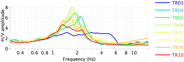
FIGURE 8. HVNSR curves of the eastern part of Section 6. The colors reported in the legend correspond to stations located from east (blue) to west (red) of the section, moving from the outcropping bedrock (almost a flat HVNSR average curve) toward the center of the valley (f0 from 2.5 to 1.5 Hz).
Taking into account that, from available geophysical investigations (multichannel analysis of surface waves) performed on the alluvial fan area (Palombelli, 2014), the average Vs for the shallow depths is around 500 m/s; we can say that the average depth of the Vallelonga valley is between 100 and 150 m. Another interesting observation is that the only three measurements which have a flat HVNSR shape (CMP2, CMP4, and CMP5) are in the central part of Section 6. They then have a similar response in terms of HVNSR as that of the rock sites, suggesting that the presence of alluvial fans can result in deep layers with shear-wave velocities lower than the ones above them (e.g., velocity inversions). In these cases, the capability of the HVNSR technique to retrieve the real resonance frequency of the area is really poor, as also shown by Castellaro and Mulargia, (2009).
Sections 7–8 are both NW-SE oriented and located in the hanging-wall and foot-wall of the Trasacco fault, respectively. They show a similar trend of deepening toward the north but the presence of the structural high in Section 8 is reflected in higher f0 values in the north-western part of the section than Section 7. On the contrary, Section 9 is SW-NE oriented, crossing perpendicularly the main fault structures as reported for the area in the ITHACA database. In this contour-plot is evident that there is a sudden deepening toward NE of the main seismic impedance contrast at around 2,800 m from the beginning of the section which corresponds to the noise measurement TF16 (see location in Figures 3, 4).
Sections 10 and 11 reported in Figure 6 (location in Figure 4) are drawn along two industrial seismic lines interpreted by Patruno and Scisciani, (2021); being particularly important, we postpone the comparison between the sections and the seismic lines afterward, in the Discussion section. However, both the sections are N-S oriented and focused on areas close to buried fault lines: in particular, Section 10 is N-S oriented, following toward the center of the basin in the eastern border of the Vallelonga valley (from FN16 to FN19 in Figure 3). A sudden decrease of the resonance frequency is reported between FN16 and FN11–FN12. Section 11 highlights a deeper seismic interface than Section 10, but ending, in its northern part, to similar frequency values.
In order to reconstruct some 1D subsoil velocity models and make inferences on the stratigraphic structure of the investigated area, we consulted public borehole log data, mostly drilled for hydrologic exploration, and few geognostic drillings made available by independent professionals. The basic level of seismic microzonation studies for the Trasacco municipality (www.webms.it) provided shallow geological and geotechnical data mainly located close to the urban area at the southern border of the FB. Other data consist of old stratigraphic logs coming from ISPRA (Italian Institute for Environmental Protection and Research) and “Ente Fucino”, a local managing institution, for old wells drilled during the ‘50s, mainly consisting of stratigraphy of water wells.
We used them to fill the lack of geological information especially where no natural outcrops were available (e.g., in the urbanized area). Unfortunately, none of the available borehole logs reached the geologic bedrock in the Trasacco municipality and the only information that we took into account was the lithology and the thickness of the deposits, just to estimate qualitatively a reasonable average shear-wave velocity of the shallower fillings of the Vallelonga valley. The presence of a large alluvial fan inside the valley represents a big issue for the interpretation of our results. The noise measurements (TF17 and TF18 belonging to Section 1, FT06 and TF13 belonging to Section 2, and TF05 and FT18 on Section 3) that are close to boreholes (green diamonds in Figure 4) with stratigraphic information (Figure 9 left) were selected to make 1D preliminary models of the subsoil with the dinver tool of Geopsy. For the area where the points are located, the availability of the borehole logs, although the description of the stratigraphic log is not very detailed (some of them were old water wells), allowed us to conclude that the sedimentation conditions are relatively simple. In fact, the shallow layer consists in strata of fine-grained sediments sometimes inter-layered by a gravelly layer (see Figure 9 for details), finally overlying a gray-clay layer. None of these boreholes reaches the depth of the geologic bedrock.
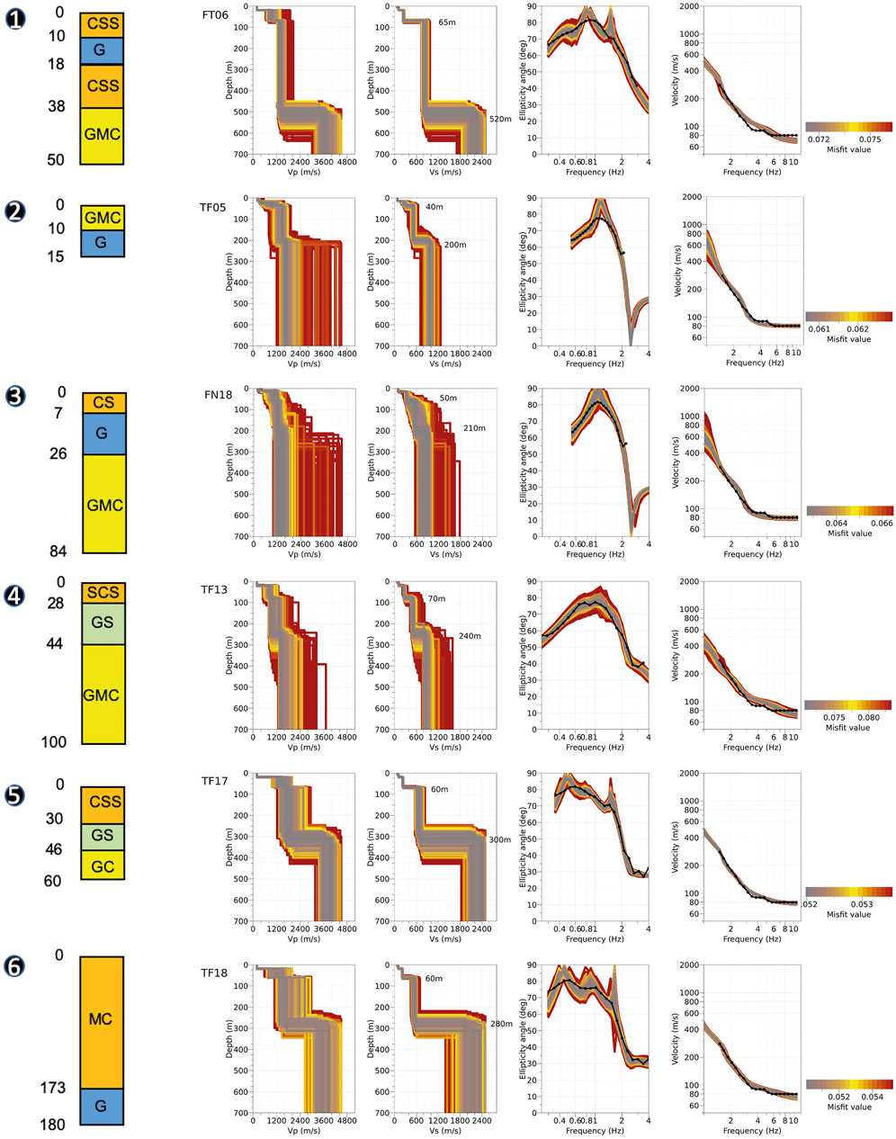
FIGURE 9. 1D models (Vp and Vs on the left) for six representative sites selected in the study area (see location in Figure 4). The target curves of the joint inversion (HVNSR considered Rayleigh-wave ellipticity and dispersion curves) are shown in black. The color scale is proportional to the misfit between experimental and theoretical curves. On the left, the borehole logs available are used to set the shallow part of the initial subsoil structure for 1D models. Legend of borehole logs: C, MC, and GMC—clay deposits; CSS, SCS, and CS—sand deposits; GS and G—gravel deposits.
The parameterization of the input subsoil starting model was designed according to the available stratigraphic logs.
The Vs models (Figure 9) obtained by joint-inverting the empirical HVNSR and the dispersion curve obtained through the cross-correlation technique (Figure 10) give an idea of the main impedance contrasts for the area. During the joint inversion, the HVNSR curve was assumed as the ellipticity of the fundamental mode of the Rayleigh wave. The inversion is able to reproduce the main features of the field curves even if in some cases the frequency trough present in the HVNSR curve is not found (e.g., for TF05 and FN18). Due to the simplified approximations of our inversion on the target curves, the 1D velocity results can be considered rough models with an increasing uncertainty at larger depths. However, we observe two main velocity contrasts in the profiles obtained from the inversion (Figure 9): the first one is found at a depth between 40 and 70 m and the second one at a depth between 200 and 520 m. From these preliminary models, we can summarize the results as follows:
1) TF05, FN18, and TF13 sites seem to be located on a structural high with a main impedance contrast located less than 250 m below the ground surface;
2) TF17 and TF18 are in an intermediate setting, with the depth of the main interface being between 280 and 300 m;
3) FT06 is outside the structural high, with a deep interface at 500 m.
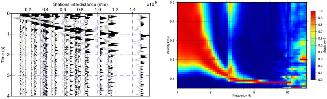
FIGURE 10. Cross-correlation of the ambient noise of synchronous HVNSR measurements in the northern part of the Trasacco area (Section 1).
The directional analysis of HVNSR can highlight the possible 2D or 3D effects in the site response of some noise measurements. We explored specific features of these analyses trying to correlate them with other geological and geophysical information, retrieved from other studies. In particular, we focused on the points closer to the uncertain tectonic elements of the investigated area: the surface fault lines identified from the satellite imagery (ITHACA database) and the buried fault segments hypothesized by the interpretation of the seismic lines (Cavinato et al., 2002; Patacca et al., 2008; Patruno and Scisciani, 2021). The latter was useful to have an idea of the main seismic interfaces present in the area including fault lines and their mutual relations.
Directional HVNSR was computed for sites located along sections 1, 2, and 3 (Figure 4), and the results are plotted in Figures 11–13.
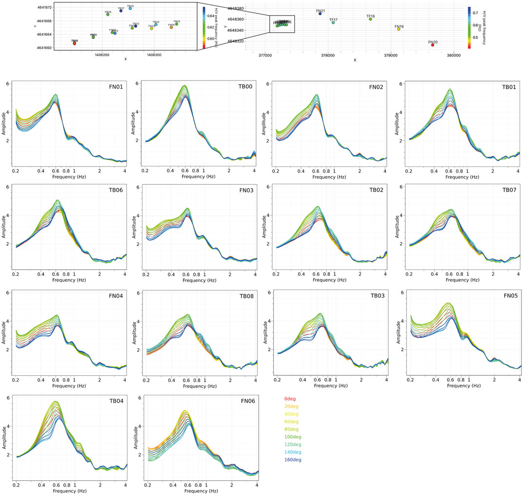
FIGURE 11. Directional HVNSR of Section 1.
For Section 3 (results in Figure 11 Figure 12 Figure 13), we observe a marked azimuthal dependence of the resonance frequency; moving from 80 to 170°, we notice a change in the f0 value from 0.85 to 1.2 Hz, respectively, for site TF08. A similar behavior is observed for stations FT06 and FT07 for Section 2 (results in Figure 12); moreover, in this case, the stations between TF12 and TF15 show a second peak close to the fundamental one not justifiable with abrupt changes of the stratigraphy.
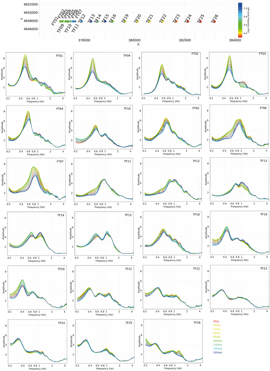
FIGURE 12. Directional HVNSR of Section 2.
For Section 1 (results in Figure 11 Figure 12 Figure 13), the directional analysis pointed out a clear azimuthal variation of HVNSR, for FN05 and TB04 stations, close to the Trasacco fault branch. In terms of HVNSR amplitudes, we observe at all the mentioned sites, minimum values around f0 for the azimuth parallel to the strike of the nearby fault. This is a feature also observed by Matsushima et al. (2014). Concerning the frequency of the HVNSR peaks, the results of Section 3 seem to be the clearer to interpret. In particular, the TF05 site, which is located on the structural high, shows a directional HVNSR revealed by the shift of the f0 peak from 1 Hz and the azimuth perpendicular to the strike of the fault (NW-SE direction), to the f0 peak of 1.3 Hz and the azimuth parallel to the strike of the fault. The TF08 results, conversely, highlight the opposite condition: the f0 peak value moving from values of 0.8 to 1 Hz for the azimuth parallel and perpendicular to the fault strike, respectively.
The detection of subsoil geological structures is a common goal for many geoscience disciplines. It is in general faced by integrating results coming from different geophysical techniques. The HVNSR technique is particularly effective for the estimations of the resonance frequencies of a given site and, by using independent information, for the estimations of the thickness or the average shear-wave velocity of the surface layers below the measurement point. It works well in simple geological settings, such as the sedimentary contexts, with horizontal and parallel low-velocity layers over a stiff seismic bedrock. The FB, of Quaternary age, only partially fulfills this geological simplicity, being interested by several faults, not all exactly known, that interrupt the homogeneity of the geological strata. Also, the presence of alluvial fans in large parts of the basin is a big issue for the right interpretation of HVNSR curves. In this work, we collected all the previous geological and geophysical information about the Trasacco area. This information not only drove the choice of the dense single-station noise survey but also helped in the interpretation of the HVNSR results. The starting motivation of this survey was to have an idea of the local structure of the continental basin but also to estimate the depth of the calcareous or siliciclastic bedrock. However, we were aware that the FB has a quite complex geologic setting: it has plenty of reverse and normal faults which, during their past activation, caused a relevant displacement of the geological layers and the interruption of their lateral continuity.
Nevertheless, we believe that the results of our noise survey added useful information for the subsoil reconstruction of the FB, shedding some lights on this complex topic, especially for the presence of buried structures in the basin area. The interpolation map of f0 allowed us to observe a double trend of the main impedance contrast of the subsoil. When the northern part of the study area shows a lowering of f0 values toward north (center of the basin), the f0 isolines (Figure 4) in the southern part show a slight change in the trend of the main impedance contrast which now dips toward NW; this variation can be explained by the co-presence of the Trasacco alluvial fan and the Vallelonga valley which could both locally influence the seismic response. Regarding the identity of the impedance contrast responsible for the fundamental resonance peak, we believe that it does not correspond to the top of calcareous rocks but to siliciclastic deposits, supported also by the high thickness values of flysch deposits reconstructed for the study area by Mancinelli et al. (2021).
Organizing the measurements in regular linear geometries has allowed the comparisons with the interpreted seismic lines already available in the FB. Despite a partial disagreement between the authors (Cavinato et al., 2002; Patacca et al., 2008; Patruno and Scisciani 2021) on the interpretation of some parts of the commercial seismic lines available in FB, the HVNSR curves interpolated along the sections (Figure 6) revealed similar results to what were provided by seismic reflection lines for depths compatible with the resonance frequency of the area.
The extension of the surveys to the scale of the municipality gave the chance to promptly reveal the presence of abrupt subsoil lateral heterogeneities as the presence of fault lines. This is easily proved following the f0 isolines from the map of f0 interpolation (Figure 4), and checking the trend of the HVNSR curves along the transects. Moreover, the strong azimuthal variation of HVNSR for the sites close to the tectonic elements supports their real presence where they are expected to be, as highlighted by Matsushima et al. (2014). A common feature for the HVNSR directional results is that, for sites close to tectonic structures, the spectral ratio curves display minimum amplitude around the f0 for the azimuth almost parallel to the strike of the fault. This seems to prove that the presence of lateral subsoil heterogeneities strongly influences the noise wavefield. This statement becomes more difficult to justify for TF12–TF13–TF14–TF15 sites (Section 2), where the amplitude values change for azimuth for the two HVNSR peaks which seem to be uncorrelated to the strike of the fault, maybe for a combined effect with other subsoil structures unknown so far. Concerning the azimuthal dependence of f0 peak values, while Section 1 does not show important f0 variations close to the Trasacco fault, and Section 2 is complex to interpret because of the disagreement in the structural reconstruction from commercial seismic lines which raise uncertainties in the existence and location of possible fault segments, Section 3 (HVNSR contour-plot in Figure 5 and directional HVNSR in Figure 13) leads itself to comment on that topic because its subsoil structure can be reasonably interpreted as a 2D structure. As discussed in the Results section, directional HVNSR curves for TF05 and TF08 sites (see location in Figure 3), among others, show a slight variation of the peak frequency related to the azimuth of computation. TF05, which we assume to be located on a structural high respect to the TF08 site (see Figure 9 for the numerical 1D simulation and comments in the related section), has an HVNSR curve with a lower f0 value (1 Hz) for the azimuth perpendicular to the fault strike and, conversely reaching a maximum of 1.3 Hz for the azimuth parallel to the fault. TF08 shows azimuthal dependence but with an opposite behavior in terms of f0 values changing from 0.8 to 1 Hz from azimuth parallel to perpendicular, respectively. We propose the following: these sites can be affected by the proximity of a lateral variation in terms of frequency of the resonant layer; this means that the trend of subsoil geometries for the area drives the energy of the noise wavefield. To demonstrate directional effects on HVNSR measurements, Matsushima et al. (2014) showed that performing numerical modeling in these cases can help understand the contribution of 1D versus 2D and 3D structures on the wavefield and, therefore, on the HVNSR curves.
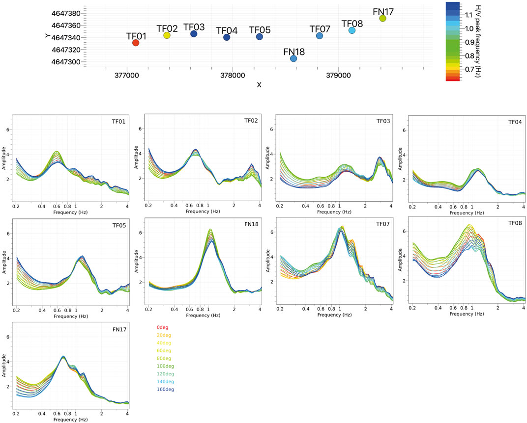
FIGURE 13. Directional HVNSR of Section 3.
Many of the noise measurements were recorded simultaneously, and gave us the opportunity to use these data to estimate the dispersion characteristics of the noise wavefield in the 1.5–10 Hz frequency range. Finally, the dispersion curve obtained using both the cross-correlation and constant velocity stack (CVS) analyses was inverted to retrieve a reliable velocity profile for the shallower layers of the western edge of Section 1. Moreover, the dispersion curve (Figure 9, right) was used, together with the HVNSR curves, as a constraint for the calculation of 1D velocity models (Figure 9) for some test sites located close to boreholes where the stratigraphy was pretty well known. Of course, this inversion process assumed that the dispersion curve obtained for the western part of Section 1 is representative of the shallow velocities of the subsoil for the entire area. We believe that this assumption is fairly realistic because it is supported by the stratigraphic logs available for the area which reflect the general homogeneity of the lithologies representative of the subsoil. However, we assigned variable depth and thickness for all the layers included the inversion process as free parameters to avoid over-constraining of the initial model. The results of these inversions in terms of velocity profiles show a variability of the depth of the main geological interface.
Finally, taking into account all the limitations of the HVNSR technique, our study has demonstrated that if this method is used as a preliminary investigation tool to identify and locate the hypothetical hidden heterogeneity, it can give some important contributions for seismic risk assessment studies, with the advantage of being an easy application and cheap when compared with other geophysical techniques. Remarkably, the HVNSR technique can give significant advancements on the geometrical reconstruction and the geological evolution of an area similar to the FB, for which extensional quaternary tectonics played an important role for its general setting. The results of this study highlight the presence of a structural high hidden by Quaternary deposits in the northern part of the Trasacco territory within the basin area. Its shape was very well constrained by the dense mesh of HVNSR measures. Another important finding is that the directional analysis for the sites of Section 2 located over this structure (from TF12 to TF15), combined with the interpretation of seismic lines and a good stratigraphic knowledge for the area, suggests that the double peak in HVNSR curves is not related to a stratigraphic effect but probably connected to the lateral heterogeneity of the subsoil.
Nevertheless, the FB has been the object of several geophysical studies in the past, and apart from some uncertainties in the precise localization, most of the hidden structures are known.
The aim of our noise measurement survey was to verify if, even in a complex context as the FB, the HVNSR technique was able to give useful information.
Our study in the Trasacco area has demonstrated that most of the HVNSR curves show a unique frequency peak (as in the 1D conditions), but the more the measurement point is close to hidden tectonic elements, the more complex the HVNSR curves become. This major complexity also affects the azimuthal variation of the HVNSR frequency peaks. The loss of continuity of the resonance peak as well as the increase of azimuthal variations are directly related to the hidden faults. Therefore, the HVNSR technique can be used as a preliminary investigation tool to reveal the presence of these hidden tectonic elements.
Therefore, the HVNSR technique has a double potential: assessing the thickness and then the geometry of the sedimentary layers, and being an indicator of potential hidden structures.
The original contributions presented in the study are included in the article/Supplementary Material; data presented in this study are available on request from the corresponding author. Further inquiries can be directed to the corresponding author.
DF: substantial contributions to the conception or design of the work, drafting the work or revising it critically for important intellectual content, acquisition, and analysis or interpretation of data for the work. FC: substantial contributions to the conception or design of the work, drafting the work or revising it critically for important intellectual content, acquisition, and analysis or interpretation of data for the work. GDG: drafting the work or revising it critically for important intellectual content, acquisition and analysis or interpretation of data for the work. MV: acquisition and analysis or interpretation of data for the work. GM: drafting the work or revising it critically for important intellectual content.
This work has been funded by MZS Avezzano livello 3 project. The authors DF, FC, GDG, and MV during part of this research work held temporary positions at INGV supported by FIRB Abruzzo - UR07 (n. RBAP10ZC8K).
The authors thank the Laboratorio Effetti di Sito (https://www.ingv.it/it/monitoraggio-e-infrastrutture-per-la-ricerca/laboratori/laboratorio-effetti-di-sito) for providing seismic equipment used in the field measurements. The authors are grateful for the insightful comments and suggestions provided by Francesco Maesano about the study area and Alessia Mercuri for providing useful suggestions with Geopsy software tools and her comments in different stages of this research project. Useful contribution to improve the paper was given by the reviewers PB and SM.
The authors declare that the research was conducted in the absence of any commercial or financial relationships that could be construed as a potential conflict of interest.
All claims expressed in this article are solely those of the authors and do not necessarily represent those of their affiliated organizations, or those of the publisher, the editors, and the reviewers. Any product that may be evaluated in this article, or claim that may be made by its manufacturer, is not guaranteed or endorsed by the publisher.
The Supplementary Material for this article can be found online at: https://www.frontiersin.org/articles/10.3389/feart.2022.937848/full#supplementary-material
Supplementary Material S1 | Average HVNSR for all the single station ambient noise measurements performed in the study area.
Supplementary Table S1 | Main parameters of the HVNSR recordings: Site Name, Lat, Lon, f0n.
Accordi, G. (1975). Nuovi affioramenti di lacustre sollevato a terrazzi al bordo settentrionale del fucino (abruzzi). Boll. Soc. Nat. Napoli 84, 1
Amoroso, S., Bernardini, F., Blumetti, A. M., Civico, R., Doglioni, C., Galadini, F., et al. (2016). Quaternary geology and paleoseismology in the fucino and L’aquila basins. Geol. Field T 8 (1.2), 1–88. doi:10.3301/GFT.2016.02
Bard, P.-Y., and Bouchon, M. (1980a). The seismic response of sediment-filled valleys. Part 1. the case of incident SH waves. Bull. Seismol. Soc. Am. 70, 1263–1286. doi:10.1785/bssa0700041263
Bard, P.-Y., and Bouchon, M. (1980b). The seismic response of sediment-filled valleys. part 2. the case of incident P and SV waves. Bull. Seismol. Soc. Am. 70 (5), 1921–1941. doi:10.1785/bssa0700051921
Bard, P.-Y., and Bouchon, M. (1985). The two-dimensional resonance of sediment-filled valleys. Bull. Seismol. Soc. Am. 75, 519–541. doi:10.1785/bssa0750020519
Bensen, G. D., Ritzwoller, M. H., Barmin, M. P., Levshin, A. L., Lin, F., Moschetti, M. P., et al. (2007). Processing seismic ambient noise data to obtain reliable broad-band surface wave dispersion measurements. Geophys. J. Int. 169 (3), 1239–1260. doi:10.1111/j.1365-246x.2007.03374.x
Blumetti, A. M., Dramis, F., and Michetti, A. M. (1993). Fault-generated mountain fronts in the central apennines (Central Italy): geomorphological features and seismotectonic implications. Earth Surf. Process. Landf. 18, 203–223. doi:10.1002/esp.3290180304
Bosi, C., Galadini, F., and Messina, P. (1995). Stratigrafia Plio-Pleistocenica della conca del fucino. Il Quat. 8 (1), 83
Cara, F., Di Giulio, G., Cavinato, G. P., Famiani, D., and Milana, G. (2011). Seismic characterization and monitoring of fucino basin (central Italy). Bull. Earthq. Eng. 9, 1961–1985. doi:10.1007/s10518-011-9282-2
Castellaro, S., and Mulargia, F. (2009). The effect of velocity inversions on H/V. Pure appl. Geophys. 166, 567–592. doi:10.1007/s00024-009-0474-5
Cavinato, G. P., Carusi, C., Dall’Asta, M., Miccadei, E., and Piacentini, T. (2002). Sedimentary and tectonic evolution of plio–pleistocene alluvial and lacustrine deposits of Fucino Basin (central Italy). Sediment. Geol. 148, 29–59. doi:10.1016/s0037-0738(01)00209-3
Cella, F., Nappi, R., Paoletti, V., and Florio, G. (2021). Basement mapping of the fucino basin in central italy by ITRESC modeling of gravity data. Geosci. (Basel). 11, 398. doi:10.3390/geosciences11100398
Di Giulio, G., Ercoli, M., Vassallo, M., and Porreca, M. (2020). Investigation of the Norcia basin (Central Italy) through ambient vibration measurements and geological surveys. Eng. Geol. 267, 105501. doi:10.1016/j.enggeo.2020.105501
Doglioni, C., Mongelli, F., and Pialli, G. P. (1998). Boudinage of the alpine belt in the apenninic back-arc. Mem. Soc. Geol. It. 52, 457
Famiani, D., Brunori, C. A., Pizzimenti, L., Cara, F., Caciagli, M., Melelli, L., et al. (2020). Geophysical reconstruction of buried geological features and site effects estimation of the middle valle umbra basin (central Italy). Eng. Geol. 269, 105543. ISSN 0013-7952. doi:10.1016/j.enggeo.2020.105543
Frezzotti, M., and Giraudi, C. (1992). Evoluzione geologica tardo-pleistocenica ed olocenica del conoide complesso della Valle Majelama (Massiccio del Velino - Abruzzo). Il Quat. 5 (1), 33
Galadini, F., Galli, P., and Giraudi, C. (1997). Geological investigations of Italian earthquakes: new paleoseismological data from the fucino plain (central Italy). J. Geodyn. 24, 87–103. doi:10.1016/s0264-3707(96)00034-8
Galadini, F., Galli, P., Giraudi, C., and Molin, D. (1995). Il terremoto del 1915 e la sismicità della piana del Fucino (Italia Centrale). Boll. Soc. Geol. It. 114, 635–663. doi:10.12910/EAI2015-075
Galadini, F., and Galli, P. (1996). Paleoseismology related to deformed archaeological remains in the fucino plain. implications for subrecent seismicity in Central Italy. Ann. Geofis. 39, 925–940. doi:10.4401/ag-4025
Galadini, F., and Galli, P. (1999). The Holocene paleoearthquakes on the 1915 Avezzano earthquake faults (central Italy): implications for active tectonics in the central apennines. Tectonophysics 308, 143–170. doi:10.1016/s0040-1951(99)00091-8
Galli, P., Messina, P., Giaccio, B., Peronace, E., and Quadrio, B. (2012). Early Pleistocene to late Holocene activity of the magnola fault (fucino fault system, central Italy). Boll. Di Geofis. Teor. Ed. Appl. 53 (4), 435–458. doi:10.4430/bgta0054
Giraudi, C. (1988). Evoluzione geologica della Piana del Fucino (Abruzzo) negli ultimi 30.000 anni. Il Quat. 1 (2), 131.
Giraudi, C. (1986). Faglie ad attività olocenica nella piana del fucino. Mem. Soc. Geol. It. 35, 875
ISPRA (1881) Geological survey of Italy. Available at: http://sgi2.isprambiente.it/ithacaweb/Mappatura.aspx.
ITHACA Working Group (2019). ITHACA (ITaly HAzard from CApable faulting), A database of active capable faults of the Italian territory. Version December 2019. ISPRA Geological Survey of Italy. Available at: http://sgi2.isprambiente.it/ithacaweb/Mappatura.aspx.
Joyner, W. B., Warrick, R. E., and Fumal, T. E. (1981). The effect of Quaternary alluvium on strong ground motion in the coyote lake, california, earthquake of 1979. Bull. Seismol. Soc. Am. 71 (4), 1333–1349. doi:10.1785/bssa0710041333
Lanari, R., Faccenna, C., Benedetti, L., Sembroni, A., Bellier, O., Menichelli, I., et al. (2021). Formation and persistence of extensional internally drained basins: The case of the Fucino basin (central apennines, Italy). Tectonics 40, e2020TC006442. doi:10.1029/2020tc006442
Lu, G. Y., and Wong, D. W. (2008). An adaptive inverse-distance weighting spatial interpolation technique. Comput. Geosciences 34 (9), 1044–1055. ISSN 0098-3004. doi:10.1016/j.cageo.2007.07.010
Mancinelli, P., Scisciani, V., Patruno, S., and Minelli, G. (2021). Gravity modeling reveals a messinian foredeep depocenter beneath the intermontane fucino basin (central apennines). Tectonophysics 821, 229144. ISSN 0040-1951. doi:10.1016/j.tecto.2021.229144
Mannella, G., Giaccio, B., Zanchetta, G., Regattieri, E., Niespolo, E. M., Pereira, A., et al. (2019). Palaeoenvironmental and palaeohydrological variability of mountain areas in the central mediterranean region: a 190 ka-long chronicle from the independently dated fucino palaeolake record (central Italy). Quat. Sci. Rev. 210, 90–210. ISSN 0277-3791. doi:10.1016/j.quascirev.2019.02.032
Mascandola, C., Massa, M., Barani, S., Albarello, D., Lovati, S., Martelli, L., et al. (2019). Mapping the seismic bedrock of the po plain (Italy) through ambient-vibration monitoring. Bull. Seismol. Soc. Am. 109 (1), 164–177. doi:10.1785/0120180193
Matsushima, S., Hirokawa, T., De Martin, F., Kawase, H., and Sánchez-Sesma, F. J. (2014). The effect of lateral heterogeneity on horizontal-to-vertical spectral ratio of microtremors inferred from observation and synthetics. Bull. Seismol. Soc. Am. 104 (1), 381–393. doi:10.1785/0120120321
Messina, P. (1996). Tettonica meso pleistocenica dei terrazzi nord-orientali del Fucino (Italia centrale). Il Quat. 9 (1), 393
Michetti, A. M., Brunamonte, F., Serva, L., and Vittori, E. (1996). Trench investigations of the 1915 Fucino earthquake fault scarps (Abruzzo, Central Italy): geological evidence of large historical events. J. Geophys. Res. 101 (B3), 5921–5936. doi:10.1029/95JB02852
Nakamura, Y. (1989). A method for dynamic characteristics estimation of subsurface using microtremor on the ground surface. Q. Rep. RTRI 30 (1), 25
Oddone, E. (1915). Gli elementi fisici del grande terremoto marsicano-fucense del 13 gennaio 1915. Boll. Soc. Sismol. Ital. 19, 71
Palombelli, R. (2014). Indagini geofisiche finalizzate allo studio della microzonazione sismica nel territorio del comune di Trasacco (AQ). Dissertation. Rome, Italy: Sapienza Università di Roma.
Patacca, E., Scandone, P., Di Luzio, E., Cavinato, G. P., and Parotto, M. (2008). Structural architecture of the central apennines: interpretation of the CROP 11 seismic profile from the adriatic coast to the orographic divide. Tectonics 27, 1–36. doi:10.1029/2005tc001917
Patruno, S., and Scisciani, V. (2021). Testing normal fault growth models by seismic stratigraphic architecture: The case of the pliocene-quaternary Fucino basin (central apennines, Italy). Basin Res. 33 (3), 2118–2156. doi:10.1111/bre.12551
Schimmel, M., and Paulssen, H. (1997). Noise reduction and detection of weak, coherent signals through phase-weighted stacks. Geophys. J. Int. 130 (2), 497–505. doi:10.1111/j.1365-246x.1997.tb05664.x
Serva, L., Blumetti, A., and Michetti, A. (1986). Gli effetti sul terreno del terremoto del Fucino (13 gennaio 1915); tentativo di interpretazione dell'evoluzione tettonica recente di alcune strutture. Mem. Soc. Geol. It. 35, 893–907.
Vassallo, M., De Matteis, R., Bobbio, A., Di Giulio, G., Adinolfi, G. M., Cantore, L., et al. (2019). Seismic noise cross-correlation in the urban area of Benevento city (Southern Italy). Geophys. J. Int. 217 (3), 1524–1542. doi:10.1093/gji/ggz101
Wathelet, M. (2008). An improved neighborhood algorithm: Parameter conditions and dynamic scaling. Geophys. Res. Lett. 35, L09301. doi:10.1029/2008GL033256
Wathelet, M., Chatelain, J.-L., Cornou, C., Di Giulio, G., Guillier, B., Ohrnberger, M., et al. (2020). Geopsy: a user-friendly open-source tool set for ambient vibration processing. Seismol. Res. Lett. 91 (3), 1878–1889. doi:10.1785/0220190360
Yamanaka, H., Takemura, M., Ishida, H., and Niwa, M. (1994). Characteristics of long-period microtremors and their applicability in exploration of deep sedimentary layers. Bull. Seismol. Soc. Am. 84, 1831–1841. doi:10.1785/bssa0840061831
Yilmaz, O. (1987). Seismic data processing in investigations in geophysics, 2: Soc. Expl. Geophys, series. Editors S. M. Doherty, and E. B. Neitzel, (Texas, United States: SEG).
Keywords: microzonation, HVNSR, hidden faults, lateral heterogeneities, subsoil reconstruction
Citation: Famiani D, Cara F, Di Giulio G, Vassallo M and Milana G (2022) Detection of hidden faults within the Fucino basin from single-station ambient noise measurements: The case study of the Trasacco fault system. Front. Earth Sci. 10:937848. doi: 10.3389/feart.2022.937848
Received: 06 May 2022; Accepted: 15 July 2022;
Published: 19 August 2022.
Edited by:
Simone Barani, University of Genoa, ItalyReviewed by:
Paolo Boncio, University of Studies G. d'Annunzio Chieti and Pescara, ItalyCopyright © 2022 Famiani, Cara, Di Giulio, Vassallo and Milana. This is an open-access article distributed under the terms of the Creative Commons Attribution License (CC BY). The use, distribution or reproduction in other forums is permitted, provided the original author(s) and the copyright owner(s) are credited and that the original publication in this journal is cited, in accordance with accepted academic practice. No use, distribution or reproduction is permitted which does not comply with these terms.
*Correspondence: Daniela Famiani, ZGFuaWVsYS5mYW1pYW5pQGluZ3YuaXQ=
Disclaimer: All claims expressed in this article are solely those of the authors and do not necessarily represent those of their affiliated organizations, or those of the publisher, the editors and the reviewers. Any product that may be evaluated in this article or claim that may be made by its manufacturer is not guaranteed or endorsed by the publisher.
Research integrity at Frontiers
Learn more about the work of our research integrity team to safeguard the quality of each article we publish.