An Effective Denoising Method Based on Cumulative Distribution Function Thresholding and its Application in the Microseismic Signal of a Metal Mine With High Sampling Rate (6 kHz)

Microseismic events can be used to analyze the risk of tunnel collapse, rock burst, and other mine hazards in space and time. In practice, the artificial activities and other signals at the mining site can seriously interfere with the microseismic waveforms, reducing the signal-to-noise ratio. In this study, we propose a denoising method based on the threshold of the cumulative distribution function (CDF) of the wavelet coefficients in the wavelet domain using synchrosqueezed continuous wavelet transform (SS-CWT). First, the ratio of microseismic signal variance between two adjacent time windows is used to determine the range of background noise. Then, the microseismic signal is transformed into a wavelet domain using SS-CWT, and the threshold of wavelet coefficients at each scale is estimated based on the cumulative distribution function (CDF) of background noise. At last, a post-processing step is applied by utilizing an amplitude smoothing function, to further suppress the noise. The proposed denoising method is tested by both synthetic and filed microseismic data recorded in a metal mine. The results show that the method is effective in denoising and can improve the SNR of mine microseismic data with a high sampling rate.

Introduction

In order to monitor mine hazards, such as roof fall, collapse, and rockburst, passive microseismic monitoring technology was introduced in the mining industry (Young et al., 1992; Li et al., 2007; Hudyma and Potvin, 2010). By detecting and analyzing microseismograms, the location, magnitude, and source mechanism of microseismic events are calculated. Applying the seismological theories, the distribution of stress drops, displacements, and radiated energy can be obtained to provide basic data for the safety evaluation of surrounding environments during mining production (Yabe et al., 2015). However, in many conventional seismic methods, the SNR of microseismic data strongly affects the reliability of data and the accuracy of waveform parameters’ estimation, such as arrival time and polarity. As a result, the accuracy of microseismic location and other source parameters extracted from waveform is also influenced by the noise content. Especially for mine data, the high sampling rate and persistent human activities in the monitoring environment make complex noises being recorded and superimposed on the microseismic signal. Therefore, it is a challenging task to accurately separate microseismic signals from miscellaneous background noise. There is still a great need for developing suitable procedures that improve SNR allowing for robust seismic processing.

The noise in seismic data is divided into two categories: regular noise and random noise. Regular noise refers to the noise with a certain apparent velocity and frequency, such as surface wave, acoustic wave, secondary interference wave, multiple-wave, and 50 Hz alternating current interference. Spectral filtering is a common method for denoising noise with the specified frequency band, but it is not effective for removing noise with the same frequencies as the signal. Moreover, effective filter bands must be known in advance, and band-pass filtering inevitably distorts the signal and generates artifacts to influence the true onset time and polarity (Douglas, 1997; Scherbaum, 2001).

The microseismic data can also be denoised using multichannel methods, which are widely used in the active-source seismic community, such as predictive filtering methods (Liu et al., 2012; Liu and Chen 2013), singular spectrum analysis (Huang et al., 2015, 2016a; Zhang et al., 2016a; Zhang et al., 2016b; Zhang et al., 2016c), low-rank approximation based methods (Huang et al., 2016b; Xie et al., 2016; Chen et al., 2017; Zhou and Zhang 2017; Bai et al., 2018), dictionary learning-based methods (Chen 2017; Siahsar et al., 2017; Wu and Bai 2018a, b), and morphological filtering based method (Huang et al., 2017). The multichannel denoising methods rely on a fairly dense spatial sampling of the data. For most microseismic monitoring projects, where the number of spatial sensors is not large enough, the multichannel denoising methods are inapplicable or cannot give acceptable results. Especially, the sensors’ number in one microseismic monitoring system is relatively small, and the spatial layout is irregular. Therefore, the denoising method based on multichannel information is not suitable for denoising of mining microseismic processing.

Many effective single-channel microseismic signal denoising methods based on time-frequency transformation have been developed, such as empirical mode decomposition (EMD) (Huang et al., 1998), short-time Fourier transform (STFT) (Mousavi and Langston, 2016a), continuous wavelet transform (CWT) (Goupillaud et al., 1984; Mousavi and Langston, 2016b), S transform (ST) (Stockwell et al., 1996; Askari and Siahkoohi, 2008; Wang et al., 2010), and general S transform (GST) (Wang et al., 2015). Recently, a new signal decomposition algorithm called synchrosqueezing transform (SST) was introduced by Daubechies et al. (2011) as an alternative to EMD. The SST can produce a sparse time-frequency representation for the modulated oscillation signal. More importantly, it has better mathematical support and more adaptive performance than EMD. Synchrosqueezed continuous wavelet transform (SS-CWT) combines wavelet analysis and SST to obtain time-frequency maps with significantly improved resolution. Mousavi et al. (2016c); Mousavi and Langston (2017) applied the SS-CWT to denoise single-channel microseismic data based on a custom thresholding strategy.

Donoho and Johnstone. (1997); Donoho and Johnstone (1995) showed that the universal threshold can be obtained for Gaussian noise in the time-frequency domain, which provides a reliable basis for subsequent denoising methods in the time-frequency domain. In this article, we introduce an effective denoising method based on cumulative distribution function (CDF) thresholding in the SS-CWT domain, including the range determination of pure background noise for noise level estimation, denoising noise based on CDF thresholding, and post-processing of weight suppression. Then, we use synthetic and field data examples to test and confirm the effectiveness of the proposed algorithm. Finally, we draw some key conclusions at the end of the article.

Theoretical Background

Synchrosqueezed Continuous Wavelet Transform

Basically, the seismic data s(t) recorded by geophones contains both microseismic signal and environmental noise, which can be expressed as

$\mathit{s}\left(\mathit{t}\right)={\mathit{s}}_0\left(\mathit{t}\right)+\mathit{\eta }\left(\mathit{t}\right),(1)$

where s₀(t) is a microseismic signal, η(t) is environmental noises.

The continuous wavelet transform (CWT) of s(t) with a given mother wavelet ψ is (Daubechies, 1988; Heil and Walnut, 1989; Farge, 1992)

${\mathit{W}}_{\mathit{s}}\left(\mathit{a},\mathit{\tau }\right)=\frac{\mathbf{1}}{\sqrt{\mathit{a}}}\underset{-\infty }{\overset{+\infty }{{\displaystyle \int }}}\mathit{s}\left(\mathit{t}\right){\mathit{\psi }}^{\mathit{\ast }}\left(\frac{\mathit{t}-\mathit{\tau }}{\mathit{a}}\right)\mathit{dt,}(2)$

where ψ* represents the complex conjugate of a mother wavelet, a and τ are the scale variable and time shift, respectively.

With a flexible trade-off between time and frequency achieved by the variable length of the mother wavelet, the signal can be presented in the time-frequency domain. However, due to signal windowing and spectral leakage, the energy is spread out on a time-scale plane in the actual application, which leads to a blurred time-frequency spectrum. Hence, the synchrosqueezed transform is used here to squeeze the energy into the real instantaneous frequency of the signal, which improves the accuracy of wavelet-based transforms for frequency content estimation.

The instantaneous frequency can be estimated by the derivative of the wavelet coefficient (Auger et al., 2013):

$\mathit{\omega }\left(\mathit{a},\mathit{\tau }\right)=-\mathit{i}{\mathit{W}}_{\mathit{s}}{\left(\mathit{a},\mathit{\tau }\right)}^{-\mathbf{1}}\frac{\partial {\mathit{W}}_{\mathit{s}}\left(\mathit{a},\mathit{\tau }\right)}{2\mathit{\pi }\partial \mathit{\tau }},for\mathit{ }{\mathit{W}}_{\mathit{s}}\left(\mathit{a},\mathit{\tau }\right)\ne 0.(3)$

This allows us to convert the time-scale plane (a, τ) into the time-frequency plane (w(a, τ), τ). Also, the synchrosqueezed wavelet transform of s(t) is (Daubechies et al., 2011)

${\mathit{T}}_{\mathit{s}}\left({\mathit{\omega }}_{\mathit{l}},\mathit{\tau }\right)=\frac{\mathbf{1}}{\text{Δ}\mathit{\omega }}{\displaystyle \sum }_{{\mathit{a}}_{\mathit{k}}:\left|\mathit{w}\left({\mathit{a}}_{\mathit{k}},\mathit{\tau }\right)-{\mathit{\omega }}_{\mathit{l}}\right|\le \frac{\text{Δ}\mathit{\omega }}{2}}{\mathit{W}}_{\mathit{s}}\left({\mathit{a}}_{\mathit{k}},\mathit{\tau }\right){\mathit{a}}_{\mathit{k}}^{\frac{-3}{2}}{\left(\text{Δ}\mathit{a}\right)}_{\mathit{k}},(4)$

where ω_l is the lth discrete frequency and the center of the interval [ω_l - 1/2Δω, ω_l + 1/2Δω]. a_k is the kth scale, and Δω = ω_k - ω_k-1. The individual component s_k from the T_s can be reconstructed by integrating the coefficients over frequencies ω_l that corresponds to the kth component (Thakur et al., 2013).

The inverse transform of the SS-CWT is (Herrera et al., 2014)

$\mathit{s}\left(\mathit{t}\right)=2{\mathit{C}}_{\mathit{\psi }}^{-1}\mathit{Re}\left({\displaystyle \sum }_{\mathit{l}}{\mathit{T}}_{\mathit{s}}\left({\mathit{\omega }}_{\mathit{l}},\mathit{ t}\right)\right),(5)$

where $C_{\psi }$ is a constant, which is given in Thakur et al. (2013) depending on the mother wavelet. As an example, Figure 1 shows the transform results of a field seismic signal using SS-CWT and other classic time-frequency analyses. Compared with STFT (Figure 1B) and CWT (Figure 1C), the SS-CWT (Figure 1D) exhibits higher energy concentration in the time-frequency plane, which brings advantages in threshold-based denoising.

FIGURE 1

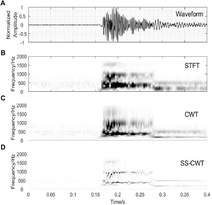
FIGURE 1. Time-frequency Spectrum of a seismic record using STFT, CWT, and SSWT. (A) Field mine microseismic signal with high SNR, the sampling rate is 6000 Hz. (B) (C), and (D) shows the STFT, CWT, and SS-CWT of the time series in (A), respectively, where CWT and SS-CWT are both based on the Morlet wavelet.

Methods

Estimation of Background Noise Range

The threshold function for denoising is determined based on the statistics of the noise. Therefore, it is important to estimate the pure background noise range accurately to obtain the threshold of each wavelet scale precisely. In the first step, the ratio of the microseismic signal variance between two adjacent time windows is proposed to determine the range of background noise. The core idea is from the conventional short-term-average (STA)/long-term-average (LTA) (Withers et al., 1998) algorithm for picking up arrival time, which utilizes the variance change of amplitude in two windows to indicate whether the presence or absence of a signal. The ratio of variance (ROV) is defined by

$\mathit{ROV}\left(\mathit{i}\right)=\frac{\mathit{var}\left({\mathit{s}}_{0,\mathit{i}}\right)}{\mathit{var}\left({\mathit{s}}_{\mathit{i},\mathit{N}}\right)},(6)$

where ROV(i) is the ratio of signal amplitude variance in two-time windows before and after the time i, var(s_{0, i}) and var(s_{i, N}) are the signal amplitude variance in two adjacent time windows, respectively. N is the length of the input data. The pure background noise range is determined according to the minimum point of ROV. Figure 2 shows an example of background noise estimation using the ROV curve. The result suggests that the ROV method can provide reliable and real-time pure background noise data, which is essential to the accurate determination of wavelet threshold for denoising in the subsequent step.

FIGURE 2

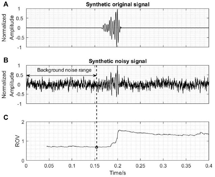
FIGURE 2. The range of background noise estimation via ROV curve. (A) The waveform of the original seismic signal. (B) Synthetic seismic signal with noise. (C) ROV curve of the synthetic noisy signal, where a black circle indicates the minimum of ROV.

Wavelet Threshold Determination Based on Cumulative Distribution Function

If the background noise obeys Gaussian distribution, the threshold function can be computed using the mean and standard deviation of the absolute value of the wavelet coefficients at each scale (Langston and Mousavi, 2019):

$\mathit{\beta }\left(\mathit{a}\right)=\mathit{mean}\left(\left|\mathit{W}(\mathit{a},\mathit{ \tau })\right|\right)+\mathit{c}\hspace{0.17em}\ast \hspace{0.17em}\mathit{st}.\mathit{dev}.\left(\left|\mathit{W}(\mathit{a},\mathit{ \tau })\right|\right),(7)$

where $\text{mean}\left(\left|W(a, \tau )\right|\right)$ and $st.dev.\left(\left|W(a, \tau )\right|\right)$ are the mean and standard deviation of wavelet coefficients at each scale a. Parameter c determines the value of wavelet coefficients threshold. It needs to be emphasized that $\beta \left(a\right)$ is computed using the pure background noise obtained in the previous step rather than the entire seismic data because the seismic signal would bias the statistic values in Eq. 7.

Donoho and Johnstone (1997) proposed a mild criterion to set the parameter c, and a widely used “universal threshold” is obtained:

$\mathit{c}=\sqrt{2\mathit{lo}{\mathit{g}}_{10}\mathit{N}},(8)$

where parameter c is related to the number of noise samples N at each scale and its value is close to 3 from this relation if N has an order of 10⁴. The threshold function will yield a confidence interval of about 99.7% for the number of noise samples N. Under such a threshold, most of the noise will be removed and about 0.3% of the noise is retained. To obtain the threshold more flexible, we take the approach of estimating the cumulative distribution function of Gaussian distribution for noise in the time window at each scale and calculating the confidence value for the distribution. The threshold function becomes

$\mathit{\beta }\left(\mathit{a}\right)=\mathit{CD}{\mathit{F}}_{\mathit{Gauss}}^{-\mathbf{1}}\left(\mathit{a}\right)\mathit{ }\left(\mathit{P}=\mathit{THRE}\right),(9)$

in which $CD{F}_{Gauss}^{-1}\left(a\right)$ is the inverse cumulative distribution function at the scale a using Gaussian distribution, and parameter THRE is the confidence value that needs to be set. Once the wavelet coefficient threshold $\beta \left(a\right)$ on each scale a is obtained, we can apply the hard thresholding method to remove noise in the time-frequency domain.

Hard thresholding is a nonlinear process. It keeps the wavelet coefficients if they are greater than a threshold criterion $\beta \left(a\right)$; otherwise, they are set to zero (Donoho and Johnstone, 1995). The denoising scheme can be expressed as follows:

$\tilde{\mathit{W}}\left(\mathit{a},\mathit{\tau }\right)=\{\begin{array}{ccc}\mathit{W}\left(\mathit{a},\mathit{\tau }\right)& \mathit{if }\left|\mathit{W}\left(\mathit{a},\mathit{\tau }\right)\right|\ge \mathit{\beta }\left(\mathit{a}\right)& \\ 0& \mathit{otherwise}& \end{array}.(10)$

Hard thresholding is known to yield abrupt artifacts in the denoised signal (Chang et al., 2000). Therefore, many scholars have developed soft thresholding functions (Weaver et al., 1991; Yoon and Vaidyanathan., 2004; Shuchong and Xun, 2014). Soft thresholding produces smaller errors but often results in oversmoothing of the denoised signal. In the next step, we add a post-processing step to smooth residual noise and minimize damage to the amplitude of the microseismic signal as much as possible.

Post-Processing

After hard thresholding in the previous step, most wavelet coefficients of noise are removed, while the wavelet coefficients of the seismic signal are almost retained. The energy of the seismic signal in the time-frequency domain exhibits higher connectivity and is numerically larger than the remaining noise. Therefore, to further suppress the noise, we construct a smoothing function, which comprehensively considers the continuity and intensity of wavelet coefficients on the time axis. To do this, the function DF is calculated by stacking the amplitude of wavelet coefficients using all scales:

$\mathit{DF}\left(\mathit{\tau }\right)={\displaystyle \sum }_{\mathit{a}=1}^{{\mathit{n}}_{\mathit{a}}}\left|\tilde{\mathit{W}}\left(\mathit{a},\mathit{\tau }\right)\right|\mathbf{for}\mathit{\tau }=\mathrm{1},\cdots ,\mathit{N},(11)$

where $n_a$ is the number of scales. Then, the smoothing function SF is calculated using DF:

$\mathit{SF}\left(\mathit{\tau }\right)=\mathbf{1}-{\left[\mathbf{1}-\mathit{exp}\left(-\frac{\mathit{\lambda }\left|\mathit{\tau }-{\mathit{\tau }}_{\mathit{m}}\right|}{\mathit{N}}\right)\right]}^{\mathit{\alpha }\frac{\mathit{DF}\left(\mathit{\tau }\right)}{\mathit{D}{\mathit{F}}_{\mathit{m}}}},(12)$

where $D{F}_m$ is the maximum of the function DF, and ${\tau }_m$ is the time position of $D{F}_m$ on the time series with length N. Parameters α and λ are nonnegative and used to adjust the importance of time distance $\left|\tau -{\tau }_m\right|$ and the ratio of the wavelet coefficient energy $DF\left(\tau \right)/D{F}_m$. If α is close to 0, the smoothing function mainly is dependent on the $\left|\tau -{\tau }_m\right|$ value; If λ is close to 0, the value $DF\left(\tau \right)/D{F}_m$ plays a dominant role in the smoothing function. The value of parameters α and λ should not be large so that the amplitude of the arrival waveform will be retained as much as possible. Notice that the smoothing function $SF\left(\tau \right)$ is only relative to time $\tau$ and independent of scale a. Therefore, the smoothing function is used to uniformly suppress the wavelet coefficients of the residual noise on all scales. An advantage of the proposed smoothing method is that the maximum amplitude of the microseismic event signal is not affected, which can improve the accuracy of mine local magnitude (M_L) calibration that utilizes the maximum amplitude information of the seismic signal.

Results

We first apply the method to synthetic data. In this way, the shape of the whole output signal can be compared with the theoretical signal. Then, the algorithm will be applied to observed microseismograms in a metal mine. In the synthetic data test, we will show the denoising performance of this method by comparing the information of phase-arrival shapes, root-mean-square error (RMS), SNR, and cross-correlation coefficients (CC) between the denoised and original signal. The SNR is measured as the ratio of the root-mean-square amplitude in a time window around the signal to that in the same length window of preceding noise. On the other hand, because the theoretical signal of the observed data in the mine is not known, we will compare the sensitivity of the onset pick-up threshold setting before and after signal denoising using a 2D microseismic event signal detector composed of STA/LTA and kurtosis algorithms. The lower the sensitivity of the microseismic event recognition threshold, the less likely it is to be misidentified.

Synthetic Data Test

The denoising algorithm is applied to a known synthetic signal and the original signal is from the field data with high SNR (Figure 2A). Then, the complex noise including the random and a fixed frequency of 50 Hz is added to the original signal to yield the resulting noisy signal with an SNR of 2.9072 (Figure 2B). According to the previous description of the denoising process, the pure background noise range should be estimated at first. Figure 3B shows that the ROV curve of the noisy signal and the range of pure background noise in a noisy signal is accurately obtained according to the minimum position of the curve, which indicates that the pure background noise estimation method we proposed is highly feasible. Then, the noisy signal is transformed into the time-frequency domain using SS-CWT and the wavelet coefficients at all scales are estimated using the hard thresholding rule of Eq. 10, scale-by-scale. In this step, the threshold function $\beta \left(a\right)$ is determined using Eq. 9, where the parameter THER is set to 99.9%, meaning the 99.9% confidence value for the distribution in the time window at each scale. The hard thresholding denoised result is shown in Figure 3C. Compared with the denoising result using the universal threshold of Donoho and Johnstone (1997) (Figure 5D), it can be seen that the wavelet coefficients of residual noise in the time-frequency spectrum of Figure 3C are less. Finally, the smoothing function of Eq. 12 is applied to smooth the CDF thresholding signal to yield the final denoising signal as shown in Figure 3D. For the waveform after denoising, the SNR is significantly improved because the noise before and after the microseismic signal is effectively removed. In the denoising time-frequency spectrum, the isolated noisy coefficients remaining after the previous steps are cleaned up and the wavelet coefficients of the signal are retained completely.

FIGURE 3

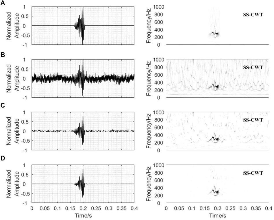
FIGURE 3. Results of each step on denoising. (A) Synthetic original signal’s waveform and SS-CWT spectrogram. (B) Synthetic noisy signal waveform and SSWT spectrogram. (C) Denoising waveform and SS-CWT spectrogram after CDF thresholding. (D) Denoising waveform and SS-CWT spectrogram after post-processing.

The goal of the denoising algorithm is to observe the effects of the denoised process on the polarity, the onset time, and smoothing of very small emergent arrivals at the very beginning of the signal buried under the background noise and track the change in other parts more easily. We compare the denoised waveform with the original waveform as shown in Figure 4A. The denoised and synthetic signals match very well over the entire waveform, especially the onset and polarity are preserved very well. The arrival time that was buried under the noise became clear after denoising, which improves arrival time picking and further benefits the source location estimation. This is greatly significant to the mining microseismic monitoring which needs a high-precision location. Comparing SS-CWT spectrums in Figures 4A,B, the noise energy is completely extracted without destroying the signal energy, which can provide reliable noise information for background noise imaging research.

FIGURE 4

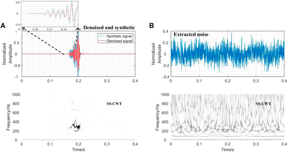
FIGURE 4. (A) Denoised seismogram and its associated SS-CWT. (B) Extracted noise and its associated SS-CWT.

The superior performance of the CDF thresholding compared with other methods commonly used is clearly shown in Figure 5. A detailed observation of the useful information of the first arriving waveform (arrival time and polarity direction of the onset) illustrates the good performance of the proposed denoising method when compared with the band-pass filtering, hard and soft thresholding. Band-pass filtering removes noise with frequencies higher and lower than the signal’s frequency range but noise within the frequency range of the signal is untouched (Figure 5C). Soft and hard thresholding preserve the structure of the signal, whereas they were much less effective in noise removal (Figures 5D,E).

FIGURE 5

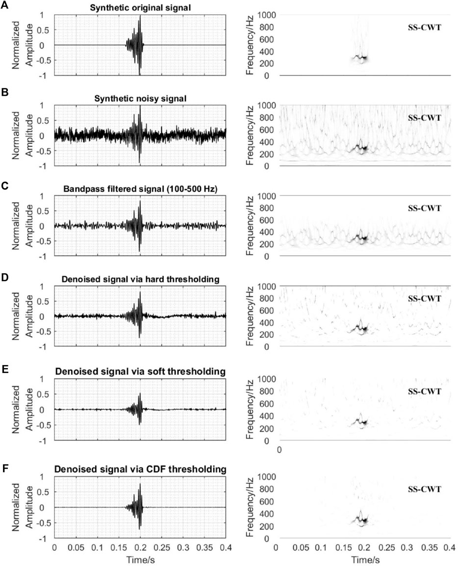
FIGURE 5. (A) The original seismic data and its SS-CWT spectrogram. (B) The synthetic noisy data and its SS-CWT spectrogram. (C) Waveform and SS-CWT spectrogram of denoised data after band-pass filtering (100–500 Hz). (D) Waveform and SS-CWT spectrogram after hard thresholding. (E) Waveform and SS-CWT spectrogram of denoised data after soft thresholding. (F) Waveform and SS-CWT spectrogram after CDF thresholding and post-processing.

The good performance of the CDF thresholding method can be further confirmed by quantitative comparative analysis of the RMS, SNR, and cross-correlation values between the denoised and original waveforms presented in Table 1. In this table, the CDF thresholding method has the smallest RMS (0.0326), the highest SNR (79.1576), and the maximal CC (0.9731) compared with the band-pass filtering and hard and soft thresholding. In terms of computational time, the CDF thresholding method takes more time to work, but it is acceptable.

TABLE 1

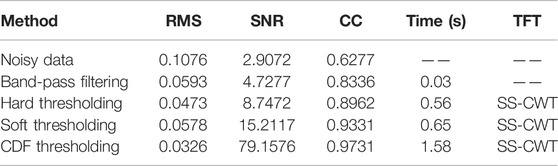
TABLE 1. Comparison of RMS, SNR, CC, and time cost among different denoising approaches.

Mine Microseismic Data

Complex background noise removal is a challenging task encountered in microseismic monitoring, especially in mine. The main reason is that the monitoring scope is small relative to the mine, so it’s necessary to accurately identify and pick up the arrival time of the microseismic signal to get the accurate source location for seismicity analysis. Therefore, the sampling rate of the microseismic record needs to be high enough to capture the microseismicity. However, the high sampling rate simultaneously makes the microseismic event more susceptible to burry in diverse environmental noise. We apply the CDF thresholding to passively recorded, complex noise mine microseismic data with different SNR to test the performance of this method in denoising and automatic detection.

Field microseismic data was recorded by seismometers of high sampling rate (6 kHz) trigger-based network operation located at a metal mine in Xinjiang, China (Figure 6). The amplitude-frequency response curve of the seismometer is shown in Figure 7. The denoising frequency band is chosen as 10–1000 Hz because the amplitude-frequency response is stable in this frequency range.

FIGURE 6

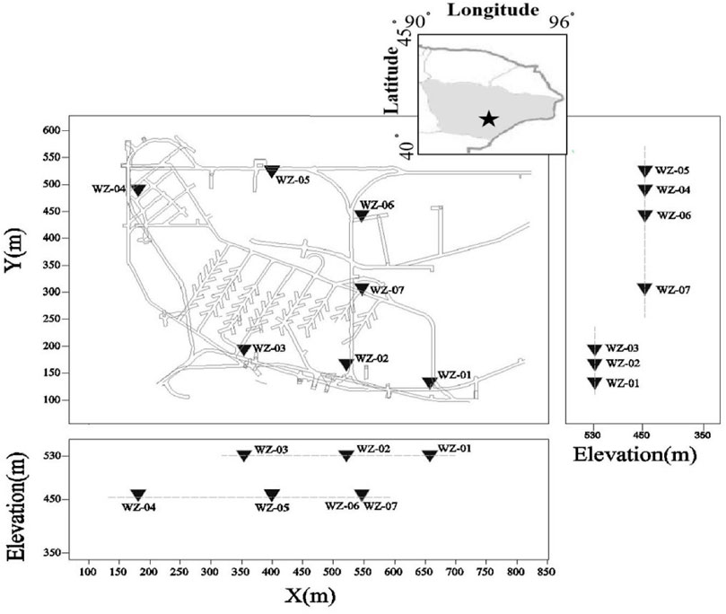
FIGURE 6. A metal mine microseismic monitoring network in Xinjiang, China, shown in one horizontal (XY) and two vertical depth sections (XZ and ZY) views. Dark inverted triangles are triggered-based seismometers.

FIGURE 7

FIGURE 7. Amplitude-frequency response curve of the seismometer utilized in the metal mine microseismic monitoring network in Xinjiang, China.

The denoising results of microseismic signals with different SNRs using the CDF thresholding are shown in Figure 8. The comparison of microseismic signals before and after denoising are from time, time-frequency, and Fourier amplitude domains. For the waveform in the time domain, the SNR of the denoised microseismic signals has been significantly improved. This can facilitate the picking of the first arrival times and their polarity which has special importance for the source location and fracture imaging. Thus, denoising microearthquakes can help to improve the detection, location, and understanding of wave propagation, which are crucial steps in microseismic processing. Comparing the signals before and after denoising in the time-frequency domain, the frequency band of the noise is almost consistent with the signal, which leads to the failure of the frequency band filtering method. The CDF thresholding method does not only cleanly remove the noise in the same frequency band as the signal, but also cleans the current interference noise of 50 Hz (Figure 8A) and the strong interference noise with multiples of 50 Hz (Figures 8B,C).

FIGURE 8

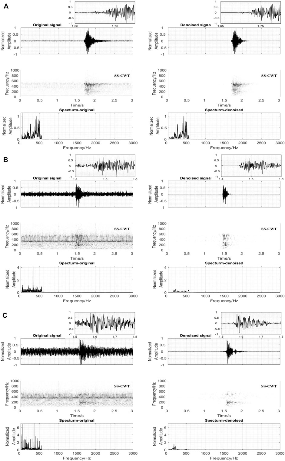
FIGURE 8. Denoised results for mining-induced microseismic records of (A) high (B) moderate, and (C) low SNR using the proposed method.

To further demonstrate the effectiveness of denoising, the performance of automatic detection is investigated. The STA/LTA (Withers et al., 1998) and kurtosis characterization function (Saragiotis et al., 2002) are combined, forming a 2D detector, which allows identifying time windows that potentially contain signals corresponding to microseismic events (Palgunadi et al., 2020). We used the training data set of 66 seismic events and 66 pure noise records to determine threshold values for this 2D detector. We recorded the maximum values of STA/LTA and kurtosis characterization functions in each event and each pure background noise time window, respectively. The result of the training data set before and after denoising is presented in Figure 9. The optimal threshold values of the original data set are around 2 and 5 for STA/LTA and kurtosis characterization function before denoising, respectively. For the denoised data set, the optimal threshold values are around 6.5 and 100. In the automatic detection procedure, any time window with values of STA/LTA and kurtosis characterization function above the two thresholds is taken as containing a microseismic event (gray rectangle in Figures 9A,B). As shown in Figure 9A, the adjustable threshold range of the original data set is narrower, implying that the automatic detection results in Figure 9A are much more sensitive to the thresholds than that in Figure 9B. This suggests that the proposed denoising method could improve the robustness of the automatic detection of microseismic events.

FIGURE 9

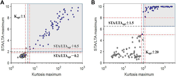
FIGURE 9. Comparison of the robustness of automatic microseismic event detection before and after denoising. White dots indicate noise measurements, blue dots correspond to microseismic events. (A) Results of Original training data set, dark dashed lines indicate the selected optimal threshold level of maximum kurtosis (K_opt=5), and maximum STA/LTA (STA/LTA_opt=2), and red dashed lines indicate the selected optimal threshold level range of kurtosis (K_opt ± 1) and STA/LTA (STA/LTA_opt - 0.2 and STA/LTA_opt + 0.5). (B) Results of denoising data set, dark dashed lines indicate the selected optimal threshold level of maximum kurtosis (K_opt=100), and maximum STA/LTA (STA/LTA_opt = 6.5), red dashed lines indicate the selected optimal threshold level range of kurtosis (K_opt ± 20) and STA/LTA (STA/LTA_opt ± 1.5).

Discussion

The first step in the denoising process is to estimate the pure background noise range, which is extremely important to the entire denoising process, as the universal threshold is related to the statistical characteristics of the background noise. In practice, the noise and seismic signals mix up with each other, and it is very difficult to accurately tell when the seismic signal arrives before denoising. The proposed ROV method can be used to obtain the pure background noise closest to the microseismic signal, providing a real-time noise estimation. This theoretically enables a more precise threshold estimation of noise and increases the denoising efficiency in the following step.

The smoothing function in the post-processing step has two nonnegative parameters. Parameter λ adjusts the weights of time distance $\left|\tau -{\tau }_m\right|$ and parameter α modulates the decay rates according to the ratio of the wavelet coefficient energy $DF\left(\tau \right)/D{F}_m$. SF increases with λ and decreases with α. The two parameters are trained by a group of the synthetic data set, and their values are between 1 and 10. The denoising results are not sensitive to the values of the two parameters, suggesting the robustness of the proposed smoothing function. Our denoising method cannot preserve the amplitude of the entire seismic signal. However, the smoothing value is equal to 1 when $\tau ={\tau }_m$, where ${\tau }_m$ represents the position of the maximum amplitude of the microseismic signal. The smoothing function can preserve the maximum amplitude of the microseismic signal. Because local magnitude (M_L) calibration utilizes the maximum amplitude information of seismic signal, the preserved maximum amplitude after denoising benefits improves the accuracy of M_L. This is crucial for subsequent seismic risk assessment.

As shown in Figure 4, wavelet coefficients of the seismic signal can be accurately separated from the noisy data without changing the time-frequency structure of the background noise using the proposed method. This provides a useful way for extracting background noise, which is crucial to dispersion curve measurement and surface wave inversion from ambient noise (Bensen et al., 2007; Wang et al., 2019).

Conclusion

We propose a new denoising framework for complex noise removal based on CDF thresholding in the SS-CWT domain. The denoising method includes the estimation of pure background noise range, determination of thresholding function based on CDF, coefficient thresholding process for wavelet coefficient, and post-processing with smooth function. Performance on both synthetic and field data demonstrates the effectiveness of the denoising method. After denoising by the proposed method, the automatic seismic detection results become less sensitive to the detector threshold, suggesting the practical value of the denoising method in handling microseismic data with a high sampling rate.

Data Availability Statement

The original contributions presented in the study are included in the article/Supplementary Material; further inquiries can be directed to the corresponding author.

Author Contributions

Conceptualization: DZ, PH, and ZZ; methodology: ZZ and PH; software: ZZ; validation: DZ, ZZ, YS, YC, RD, HJ, and PH; formal analysis: ZZ; investigation: ZZ and PH; resources: DZ; data curation: DZ, ZZ, and PH; writing—original draft preparation: ZZ; writing—review and editing: ZZ, YC, DZ, and PH; visualization: ZZ; and supervision: DZ and PH. All authors have read and agreed to the published version of the manuscript.

Funding

This research was partly supported by the National Key Research & Development Program of China (2018YFE0121000 and 2020YFE0202800), Key Special Project for Introduced Talents Team of Southern Marine Science and Engineering Guangdong Laboratory (Guangzhou) (GML2019ZD0203), and Shenzhen Key Laboratory of Deep Offshore Oil and Gas Exploration Technology (Grant No. ZDSYS20190902093007855).

Conflict of Interest

The authors declare that the research was conducted in the absence of any commercial or financial relationships that could be construed as a potential conflict of interest.

Publisher’s Note

All claims expressed in this article are solely those of the authors and do not necessarily represent those of their affiliated organizations, or those of the publisher, the editors, and the reviewers. Any product that may be evaluated in this article, or claim that may be made by its manufacturer, is not guaranteed or endorsed by the publisher.

Acknowledgments

The microseismic data are from the Institute of Mining Engineering, BGRIMM Technology Group, Beijing, China.

References

Askari, R., and Siahkoohi, H. R. (2008). Ground Roll Attenuation Using the S and X-F-K Transforms. Geophys. Prospect 56, 105–114. doi:10.1111/j.1365-2478.2007.00659.x

CrossRef Full Text | Google Scholar

Auger, F., Flandrin, P., Lin, Y.-T., McLaughlin, S., Meignen, S., Oberlin, T., et al. (2013). Time-frequency Reassignment and Synchrosqueezing: An Overview. IEEE Signal Process. Mag. 30, 32–41. doi:10.1109/MSP.2013.2265316

CrossRef Full Text | Google Scholar

Bai, M., Wu, J., Xie, J., and Zhang, D. (2018). Least-squares Reverse Time Migration of Blended Data with Low-Rank Constraint along Structural Direction. J. Seismic Explor. 27 (1), 29–48.

Google Scholar

Bensen, G. D., Ritzwoller, M. H., Barmin, M. P., Levshin, A. L., Lin, F., Moschetti, M. P., et al. (2007). Processing Seismic Ambient Noise Data to Obtain Reliable Broad-Band Surface Wave Dispersion Measurements. Geophys. J. Int. 169(3), 1239–1260.doi:10.1111/j.1365-246X.2007.03374.x

CrossRef Full Text | Google Scholar

Chang, S. G., Bin YuYu, B., and Vetterli, M. (2000). Adaptive Wavelet Thresholding for Image Denoising and Compression. IEEE Trans. Image Process. 9, 1532–1546. doi:10.1109/83.862633

PubMed Abstract | CrossRef Full Text | Google Scholar

Chen, Y. (2017). Fast Dictionary Learning for Noise Attenuation of Multidimensional Seismic Data. Geophys. J. Int. 209, 21–31. doi:10.1093/gji/ggw492

CrossRef Full Text | Google Scholar

Chen, Y., Zhou, Y., Chen, W., Zu, S., Huang, W., and Zhang, D. (2017). Empirical Low-Rank Approximation for Seismic Noise Attenuation. IEEE Trans. Geosci. Remote Sens. 55 (8), 4696–4711. doi:10.1109/TGRS.2017.2698342

CrossRef Full Text | Google Scholar

Daubechies, I., Lu, J., and Wu, H.-T. (2011). Synchrosqueezed Wavelet Transforms: An Empirical Mode Decomposition-like Tool. Appl. Comput. Harmon. Analysis 30 (2), 243–261. doi:10.1016/j.acha.2010.08.002

CrossRef Full Text | Google Scholar

Daubechies, I. (1998). Orthonormal Bases of Compactly Supported Wavelets. Commun. Pure Appl. Math. 41, 909–996. doi:10.1002/(ISSN)1097-0312

CrossRef Full Text | Google Scholar

Donoho, D. L., and Johnstone, I. M. (1995). Adapting to Unknown Smoothness via Wavelet Shrinkage. J. Am. Stat. Assoc. 90 (432), 1200–1224. doi:10.1080/01621459.1995.10476626

CrossRef Full Text | Google Scholar

Donoho, D. L., and Johnstone, I. M. (1994). Ideal Spatial Adaptation by Wavelet Shrinkage. Biometrika 81, 425–455. doi:10.1093/biomet/81.3.425

CrossRef Full Text | Google Scholar

Douglas, A. (1997). Bandpass Filtering to Reduce Noise on Seismograms: Is There a Better Way? Bull. Seismol. Soc. Am. 87, 770–777. doi:10.1785/BSSA0870030770

CrossRef Full Text | Google Scholar

Farge, M. (1992). Wavelet Transforms and Their Applications to Turbulence. Annu. Rev. Fluid Mech. 24, 395–458. doi:10.1146/annurev.fl.24.010192.002143

CrossRef Full Text | Google Scholar

Goupillaud, P., Grossmann, A., and Morlet, J. (1984). Cycle-octave and Related Transforms in Seismic Signal Analysis. Geoexploration 23 (1), 85–102. doi:10.1016/0016-7142(84)90025-5

CrossRef Full Text | Google Scholar

Heil, C. E., and Walnut, D. F. (1989). Continuous and Discrete Wavelet Transforms. SIAM Rev. 31, 628–666. doi:10.1137/1031129

CrossRef Full Text | Google Scholar

Herrera, R. H., Han, J., and van der Baan, M. (2014). Applications of the Synchrosqueezing Transform in Seismic Time-Frequency Analysis. Geophysics 79 (3), V55–V64. doi:10.1190/geo2013-0204.1

CrossRef Full Text | Google Scholar

Huang, N. E., Shen, Z., Long, S. R., Wuau, M. C., Shihau, H. H., Zhengau, Q., et al. (19981971). The Empirical Mode Decomposition and the Hilbert Spectrum for Nonlinear and Non-stationary Time Series Analysis. Proc. R. Soc. Lond. A 454, 903–995. doi:10.1098/rspa.1998.0193

CrossRef Full Text | Google Scholar

Huang, W., Wang, R., Chen, X., Zhou, Y., Chen, Y., and You, J. (2017). “Lowfrequency Noise Attenuation of Seismic Data Using Mathematical Morphological Filtering,” in 87th Annual International Meeting, SEG, Expanded Abstracts, Houston, Texas, September 28, 2017, 5011–5016. doi:10.1190/segam2017-17665921.1

CrossRef Full Text | Google Scholar

Huang, W., Wang, R., Chen, Y., Yuan, Y., and Zhou, Y. (2016a). “Randomizedorder Multichannel Singular Spectrum Analysis for Simultaneously Attenuating Random and Coherent Noise,” in 86th Annual International Meeting SEG Expanded Abstracts, Dallas, Texas, October 16–21, 2016, 4777–4781. doi:10.1190/segam2016-13859407.1

CrossRef Full Text | Google Scholar

Huang, W., Wang, R., Zhang, M., Chen, Y., and Yu, J. (2015). “Random Noise Attenuation for 3D Seismic Data by Modified Multichannel Singular Spectrumanalysis.” in 77th Annual International Conference and Exhibition, EAGE, Extended Abstracts. IFEMA Madrid, Spain, 1-4 June 2015.doi:10.3997/2214–4609.201412830

CrossRef Full Text | Google Scholar

Huang, W., Wang, R., Zhou, Y., Chen, Y., and Yang, R. (2016b). “Improved Principal Component Analysis for 3D Seismic Data Simultaneous Reconstruction and Denoising,” in 86th Annual International Meeting SEG Expanded Abstracts, Dallas, Texas, October 18, 2016, 4777–4781. doi:10.1190/segam2016-13858769.1

CrossRef Full Text | Google Scholar

Hudyma, M., and Potvin, Y. H. (2010). An Engineering Approach to Seismic Risk Management in Hardrock Mines. Rock Mech. Rock Eng. 43 (6), 891–906. doi:10.1007/s00603-009-0070-0

CrossRef Full Text | Google Scholar

Langston, C. A., and Mousavi, S. M. (2019). Separating Signal from Noise and from Other Signal Using Nonlinear Thresholding and Scale-Time Windowing of Continuous Wavelet Transforms. Bull. Seismol. Soc. Am. 109 (5), 1691–1700. doi:10.1785/0120190075

CrossRef Full Text | Google Scholar

Li, T., Cai, M. F., and Cai, M. (2007). A Review of Mining-Induced Seismicity in China. Int. J. Rock Mech. Min. Sci. 44 (8), 1149–1171. doi:10.1016/j.ijrmms.2007.06.002

CrossRef Full Text | Google Scholar

Liu, G., Chen, X., Du, J., and Wu, K. (2012). Random Noise Attenuation Using F-X Regularized Nonstationary Autoregression. Geophysics 77 (2), V61–V69. doi:10.1190/geo2011-0117.1

CrossRef Full Text | Google Scholar

Liu, G., and Chen, X. (2013). Noncausal F-X-Y Regularized Nonstationary Prediction Filtering for Random Noise Attenuation on 3D Seismic Data. J. Appl. Geophys. 93, 60–66. doi:10.1016/j.jappgeo.2013.03.007

CrossRef Full Text | Google Scholar

Mousavi, S. M., and Langston, C. A. (2016a). Adaptive Noise Estimation and Suppression for Improving Microseismic Event Detection. J. Appl. Geophys. 132, 116–124. doi:10.1016/j.jappgeo.2016.06.008

CrossRef Full Text | Google Scholar

Mousavi, S. M., and Langston, C. A. (2017). Automatic Noise-Removal/signal-Removal Based on General Cross-Validation Thresholding in Synchrosqueezed Domain and its Application on Earthquake Data. Geophysics 82 (4), V211–V227. doi:10.1190/geo2016-0433.1

CrossRef Full Text | Google Scholar

Mousavi, S. M., Langston, C. A., and Horton, S. P. (2016c). Automatic Microseismic Denoising and Onset Detection Using the Synchrosqueezed Continuous Wavelet Transform. Geophysics 81 (4), V341–V355. doi:10.1190/geo2015-0598.1

CrossRef Full Text | Google Scholar

Mousavi, S. M., and Langston, C. A. (2016b). Hybrid Seismic Denoising Using Higher‐Order Statistics and Improved Wavelet Block Thresholding. Bull. Seismol. Soc. Am. 106, 1380–1393. doi:10.1785/0120150345

CrossRef Full Text | Google Scholar

Nazari SiahsarSiahsar, M. A., Gholtashi, S., Kahoo, A. R., Chen, W., and Chen, Y. (2017). Data-driven Multitask Sparse Dictionary Learning for Noise Attenuation of 3D Seismic Data. Geophysics 82 (6), V385–V396. doi:10.1190/geo2017–0084.110.1190/geo2017-0084.1

CrossRef Full Text | Google Scholar

Palgunadi, K. H., Poiata, N., Kinscher, J., Bernard, P., De Santis, F., and Contrucci, I. (2020). Methodology for Full Waveform Near Real-Time Automatic Detection and Localization of Microseismic Events Using High (8 kHz) Sampling Rate Records in Mines: Application to the Garpenberg Mine (Sweden). Seismol. Res. Lett. 91 (1), 399–414. doi:10.1785/0220190074

CrossRef Full Text | Google Scholar

Saragiotis, C. D., Hadjileontiadis, L. J., and Panas, S. M. (2002). PAI-S/K: A Robust Automatic Seismic P Phase Arrival Identification Scheme. IEEE Trans. Geosci. Remote Sens. 40 (6), 1395–1404. doi:10.1109/tgrs.2002.800438

CrossRef Full Text | Google Scholar

Scherbaum, F. (2001). Of Poles and Zeros Fundamentals of Digital Seismology. 1st edn. Springer Dordrecht: Kluwer Academic Publishers.

Google Scholar

Shuchong, L., and Xun, C. (2014). Seismic Signals Wavelet Packet De-noising Method Based on Improved Threshold Function and Adaptive Threshold. Comput. Model. New Technol. 18, 1291–1296.

Google Scholar

Stockwell, R. G., Mansinha, L., and Lowe, R. P. (1996). Localization of the Complex Spectrum: the S Transform. IEEE Trans. Signal Process. 44 (4), 998–1001. doi:10.1109/78.492555

CrossRef Full Text | Google Scholar

Thakur, G., Brevdo, E., FučkarFuckar, N. S., and Wu, H.-T. (2013). The Synchrosqueezing Algorithm for Time-Varying Spectral Analysis: Robustness Properties and New Paleoclimate Applications. Signal Process. 93, 1079–1094. doi:10.1016/j.sigpro.2012.11.029

CrossRef Full Text | Google Scholar

Wang, D.-w., Li, Y.-j., Zhang, K., and Xu, H.-m. (2010). An Adaptive Time-Frequency Filtering Method for Nonstationary Signals Based on the Generalized S-Transform. Optoelectron. Lett. 6 (2), 133–136. doi:10.1007/s11801-010-9250-0

CrossRef Full Text | Google Scholar

Wang, D., Wang, J., Liu, Y., and Xu, Z. (2015). “An Adaptive Time-Frequency Filtering Algorithm for Multi-Component LFM Signals Based on Generalized S-Transform,” in 21st International Conference on Automation and Computing (ICAC), Glasgow, UK, 11-12 September 2015 (IEEE). doi:10.1109/iconac.2015.7314000

CrossRef Full Text | Google Scholar

Wang, J., Wu, G., and Chen, X. (2019). Frequency‐Bessel Transform Method for Effective Imaging of Higher‐Mode Rayleigh Dispersion Curves From Ambient Seismic Noise Data. J. Geophys. Res. Solid Earth 124, 3708–3723. doi:10.1029/2018JB016595

CrossRef Full Text | Google Scholar

Weaver, J. B., XuYansun, Y., Healy, D. M., and Cromwell, L. D. (1991). Filtering Noise from Images with Wavelet Transforms. Magn. Reson. Med. 21, 288–295. doi:10.1002/mrm.1910210213

PubMed Abstract | CrossRef Full Text | Google Scholar

Withers, M., Aster, R., Young, C., Beiriger, J., Harris, M., Moore, S., et al. (1998). A Comparison of Select Trigger Algorithms for Automated Global Seismic Phase and Event Detection. Bull. Seismol. Soc. Am. 88 (1), 95–106. doi:10.1785/BSSA0880010095

CrossRef Full Text | Google Scholar

Wu, J., and Bai, M. (2018b). Attenuating Seismic Noise via Incoherent Dictionary Learning. J. Geophys. Eng. 15 (4), 1327–1338. doi:10.1093/jge/aaaf57

CrossRef Full Text | Google Scholar

Wu, J., and Bai, M. (2018a). Incoherent Dictionary Learning for Reducing Crosstalk Noise in Least-Squares Reverse Time Migration. Comput. Geosciences 114, 11–21. doi:10.1016/j.cageo.2018.01.010

CrossRef Full Text | Google Scholar

Xie, J., Di, B., Wei, J., Xie, Q., Zu, S., and Chen, Y. (2016). “Stacking Using Truncated Singular Value Decomposition and Local Similarity.” in 78th Annual International Conference and Exhibition, EAGE, Extended Abstracts. Houten The Netherlands, May 2016 (European Association of Geoscientists & Engineers).doi:10.3997/2214–4609.201601325

CrossRef Full Text | Google Scholar

Yabe, Y., Nakatani, M., Naoi, M., Philipp, J., Janssen, C., Watanabe, T., et al. (2015). Nucleation Process of an M2 Earthquake in a Deep Gold Mine in South Africa Inferred from On-Fault Foreshock Activity. J. Geophys. Res. Solid Earth 120, 5574–5594. doi:10.1002/2014JB011680

CrossRef Full Text | Google Scholar

Yoon, B. J., and Vaidyanathan, P. P. (2004). “Wavelet-based Denoising by Customized Thresholding,” in International Conference on Acoustic Speech Signal Process(ICASSP), Montreal, Québec, 17-21 May 2004 (IEEE).

Google Scholar

Young, R. P., Maxwell, S. C., Urbancic, T. I., and Feignier, B. (1992). Mining-induced Microseismicity: Monitoring and Applications of Imaging and Source Mechanism Techniques. Pageoph 139, 697–719. doi:10.1007/BF00879959

CrossRef Full Text | Google Scholar

Zhang, D., Chen, Y., and Gan, S. (2016a). “Iterative Reconstruction of 3D Seismic Data via Multiple Constraints,” in 78th Annual International Conference and Exhibition, EAGE, Extended Abstracts, Houten The Netherlands, May 2016 (European Association of Geoscientists & Engineers). doi:10.3997/2214–4609.201601241

CrossRef Full Text | Google Scholar

Zhang, D., Chen, Y., and Gan, S. (2016b). “Multi-Dimensional Seismic Data Reconstruction With Multiple Constraints,” in 86th Annual International Meeting, SEG, Expanded Abstracts, Houston Texas UN, October 19, 2016 (Society of Exploration Geophysicists), 4801–4806. doi:10.1190/segam2016-13763335.1

CrossRef Full Text | Google Scholar

Zhang, D., Chen, Y., Huang, W., and Gan, S. (2016c). “Multi-step Reconstruction of 3D Seismic Data via an Improved MSSA Algorithm,” in 2016 International Geophysical Conference & Exposition, SEG, Expanded Abstracts, CPS/SEG Beijing, 745–749.

Google Scholar

Zhou, Y., and Zhang, S. (2017). Robust Noise Attenuation Based on Nuclear Norm Minimization and a Trace Prediction Strategy. J. Appl. Geophys. 147, 52–67. doi:10.1016/j.jappgeo.2017.09.005

CrossRef Full Text | Google Scholar