 Kai Liu
 Chunqiao Song
 Pengfei Zhan
 Shuangxiao Luo
94% of researchers rate our articles as excellent or good
Learn more about the work of our research integrity team to safeguard the quality of each article we publish.
Find out more
ORIGINAL RESEARCH article
Front. Earth Sci., 13 July 2022
Sec. Hydrosphere
Volume 10 - 2022 | https://doi.org/10.3389/feart.2022.925944
This article is part of the Research TopicClimatic and Associated Cryospheric and Hydrospheric Changes on the Third Pole, volume IIView all 11 articles
The widespread lakes on the Tibetan Plateau (TP) are key components of the water cycle, thus the knowledge of their spatial distribution and volume is crucial for understanding the hydrological processes under ongoing climate change. Many previous studies focus on investigating surface elevation, inundation area variations and water volume changes for these lakes. However, how much water is stored in lakes across the TP remains relatively unexplored. It is because of the incapacity of satellite remote sensing methods in lake depth measurements and the high cost of field bathymetric measurement. This study developed a low-cost approach by integrating remote sensing data and limited underwater surveys. The observed lake areas and surface elevations generated the elevation-area relationship. Underwater surveys were conducted to detect the potentially “maximum” lake depths using three optimized survey routes. With the constraint of lake-bottom elevation, the lake-bottom zone area could be estimated for calculating the lake volume. Experiments on nine TP lakes with different size and geometric characteristics demonstrate that the optimized survey line along the lake short axis is well balanced in efficiency and accuracy, with an overall volume bias of 15% approximately. The proposed hypsometric curve method coupled with the bottom elevation measurement is expected to provide a simplified but efficient solution for estimating the lake water volume on the TP, which could be applicable to ungauged lakes in other harsh environments.
Lakes play a critical part in the water cycle and provide wide-ranging ecosystem services (Pekel et al., 2016; Busker et al., 2019; Woolway et al., 2020; Liu et al., 2021b). Remote sensing observations indicated more than 100 million lakes worldwide with uneven distribution (Verpoorter et al., 2014). As one of the most concentrated areas of lake distribution, the Tibetan Plateau (TP) hosts more than 1330 lakes (>1 km2) in 2020, with a total area of ∼5 × 10⁴ km2 (Zhang et al., 2021a). Lakes on the TP are highly sensitive to climate change because of minimal disturbances from human activities. Many previous studies have examined the lake dynamics by using various remote sensing techniques (Lei et al., 2013; Yang et al., 2018; Yao et al., 2018; Li et al., 2019a; Qiao et al., 2019b; Liu et al., 2021a; Cheng et al., 2022). However, the satellite remote sensing-based studies focus on investigating variations of surface elevation, inundation area and water storage for these lakes. Lack of the underwater depths for most of the Tibetan lakes is a major obstacle for calculating absolute lake volume of this region. Thus, to answer how much water is stored in the high-altitude deep lakes of the TP is still a very challenging task due to the harsh environment and high cost of field investigation (Zhang et al., 2020).
Field measurement using the onboard sonar is the most reasonable method for generating the bathymetric map (Bandini et al., 2018; Qiao et al., 2019a; Coggins and Ghadouani, 2019). However, the labor cost and low efficiency limited the large-scale underwater lake surveys over the TP. To overcome the disadvantage of the traditional survey, some researchers attempted to derive the bathymetric map using remote sensing technologies (Getirana et al., 2018; Li et al., 2019b, 2020). Both the optical images and satellite altimetry were used to derive the underwater topography of inland or coastal waterbodies (Armon et al., 2020; Xu et al., 2022), yet being restricted in deep or turbid water conditions (Saylam et al., 2017; Bandini et al., 2018). Some spatial prediction and modeling methods were gradually proposed to overcome such difficulties mentioned above by predicting underwater bathymetry using exposed lake-surrounding terrains (Hollister et al., 2011; Heathcote et al., 2015; Cael et al., 2017; Getirana et al., 2018). For example, Messager et al. (2016) developed a geo-statistical model based on available bathymetric data of 12,150 natural lakes to estimate the lake volume globally. This approach is believed to derive reasonable results on a global scale. However, the uncertainty for lake individuals varies considerably.
Given the high cost of field measurement in full coverage and the low accuracy of the spatial prediction method for local scale, this study aims to propose an efficient method for water volume estimation for lakes on the TP. Inspired by the application of the lake hypsometric curve method in monitoring lake volume change trajectory (Yigzaw et al., 2018; Fassoni-Andrade et al., 2020; Li et al., 2021), we tried to estimate the lake volume by extrapolating the hypsometric curve fitting to the near-bottom constrained by the minimized water depth surveys. The most commonly used hypsometric curve method is to combine the water area estimations from satellite imagery (e.g., Landsat and MODIS) with elevations from altimetry datasets (e.g., Hydroweb, G-REALM, and DAHITI) (Crétaux et al., 2011; Busker et al., 2019). Recently, Li et al. (2019a) developed a novel approach to establishing the lake elevation-area (E-A) relationship by projecting the lidar-based elevation profile (i.e., ICESat-2) onto the surface water occurrence generated from long-term water classifications, and this method has been applied to the global scale (Li et al., 2020). In this study, the hypsometric curve of the lake E-A relationship was derived from the satellite observation of the historically inundated areas and corresponding water levels. Subsequently, an optimized survey line over the lake was designed for determining the bottom depths (elevations) with limited underwater surveys. The lake-bottom elevation was further used for constraining the hypsometric curve to predict the near-bottom area. Finally, after obtaining the water depth and area of the bottom zone, the lake elevation-volume (E-V) curve can be generated along with the estimated lake water volume.
The Tibetan Plateau is the highest and most extensive highland worldwide, with an average elevation exceeding 4000 m above sea leave (Chen et al., 2020). The TP is widely acknowledged as the Asian Water Tower because more than ten large rivers originate from the TP and adjacent mountain ranges (Immerzeel and Bierkens, 2012), where are distributed with about 50,000 km2 of lakes. The TP lakes are mainly concentrated in the endorheic basin and are sensitive to climate change. Many previous studies have investigated the long-term trend and spatial pattern of lake dynamics over the TP (Song et al., 2013; Li et al., 2019a). This study targets to demonstrate the approach of estimating absolute lake volume. Three items of criteria were considered in selecting the case lakes. First, the bathymetric data is available for evaluating the accuracy of lake water volume estimates. Currently, only nearly 30 lakes on the TP have open-access bathymetry. Second, the long-term satellite altimetry data can be accessed for deriving the lake level series. Last, the selected lakes should be roughly representative in the area, morphology, location, and surrounding topography. We eventually chose nine lakes based on the above-mentioned criteria, including Aksai Chin Lake, Bangda Co, Eling Lake, Manasarovar Lake, Kusai Lake, Pung Co, Tangra Yumco, Taro Co, and Zharinam Co. (Figure 1). The basic information about the case lakes is listed in Table 1.
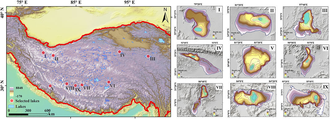
FIGURE 1. Distribution of nine selected lakes and their bathymetric data. The lakes are in order as follows: Aksai Chin Lake, Bangda Co, Eling Lake, Kusai Lake, Manasarovar Lake, Pung Co, Tangra Yumco, Taro Co, and Zharinam Co.
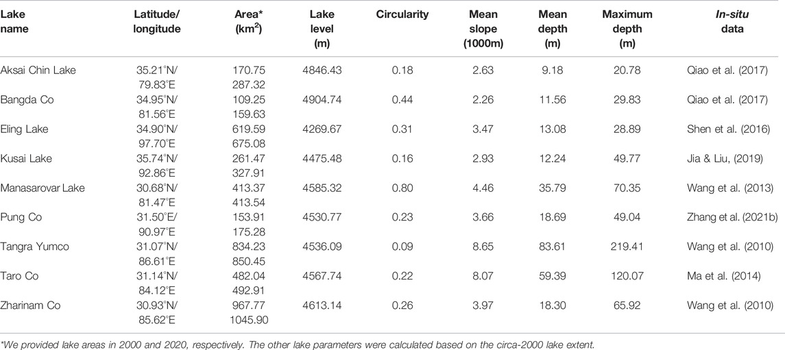
TABLE 1. Basic information of the selected lakes.
We collected the bathymetric maps of the nine case lakes from the published literature, which were generated based on full-coverage measurements using the boat-mounted depth meter. The high-quality lake bathymetry data can provide the reference data for the performance assessment of volume estimation. The hypsometric curve construction requires the paired time series of lake areas and water levels in the (near-) synchronous measurement periods. Landsat-7 ETM+ and Landsat-8 OLI images were employed for lake extent mapping. Lake level series were derived from the satellite altimetry data, including ICESat/ICESat-2 and Hydroweb dataset. In addition, the digital elevation model (DEM), which depicts the lake surrounding terrains, was also used. Among all the available DEMs over the TP, MERIT, the improved version of the SRTM DEM was selected due to its high accuracy and early acquisition time (February 2000) (Yamazaki et al., 2017; Liu et al., 2019).
This study proposes a low-cost and simplified method for lake volume estimation. As shown in Figure 2, the method includes four main steps. First, the hypsometric curve of the “Elevation-Area (E-A)” relationship was constructed based on the (near-) synchronous lake area and water level series. Next, the underwater survey was conducted along with the optimized survey line for determining the lake bottom elevation. Then, with the constraint of the lake bottom, the lake-bottom area was predicted by extending the hypsometric curve to the permanently inundated area. Last, the year 2000 was selected as the benchmark, and the total lake volume in 2000 can be estimated by calculating the volume of a frustum based on the solid geometry formula. The details of the above four steps are as follows.
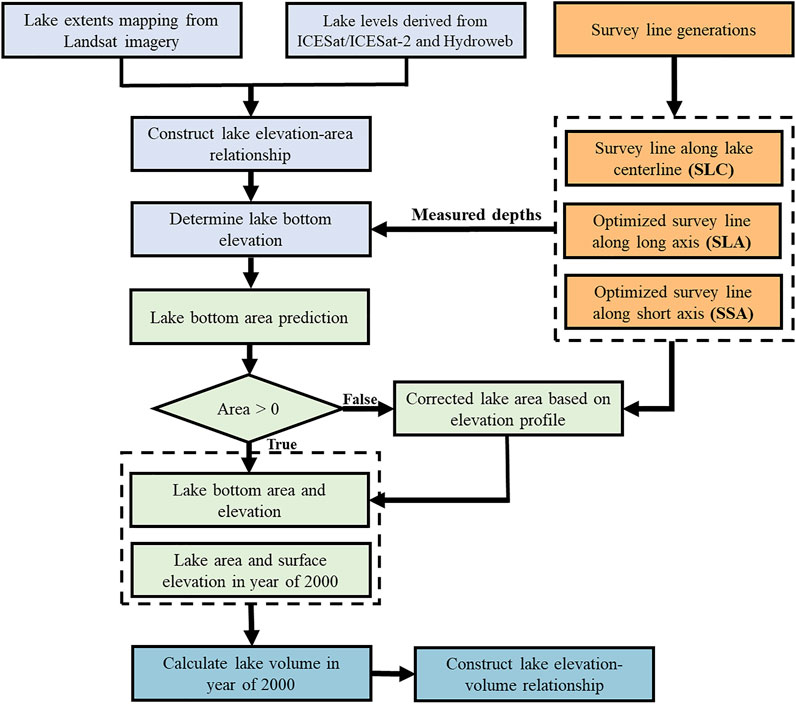
FIGURE 2. Workflow of the proposed method.
The E-A relationship is a widely-used metric for capturing the morphologic features of lakes and reservoirs, which is constructed by pairing up the lake areas and corresponding elevations (water levels) information from in-situ measurements or satellite observations. As all selected lakes are ungauged in this study, the ICESat/ICESat-2 measurements and the altimetry data provided by Hydroweb were jointly used for monitoring lake level changes. Our previous studies have revealed two-generation ICESat mission data coverage over the TP lakes (Luo et al., 2021), among which seven study lakes are included. The long-term change of these seven lakes was determined by integrating ICESat/GLAH14 and ICESat-2 ATL13 version 4 data. We collected the orthometric heights in the EGM96 datum by subtracting geoid heights from ellipsoidal heights. The other two lakes, Pung Co and Kusai Lake, have the altimetry data provided by the Hydroweb.
According to the time slots of our obtained lake levels, we collected the temporally corresponding images for mapping the lake areas. We employed the Landsat-7 ETM+ and Landsat-8 OLI images to extract multi-temporal lake inundation extents. The common-used normalized difference water index (NDWI) was applied in this study along with a two-step threshold segmentation strategy to extract the water extent area based on our previous studies (Sheng et al., 2016; Song et al., 2018). Lake mapping was performed in the Google Earth Engine platform, reducing the time cost of preparing the source imagery. After generating long-term surface elevation and surface areas, the hypsometric curves of the E–A relationship can be derived for each lake.
Water-depth measurement is necessary for this method to determine the lake-bottom elevation. However, the full-coverage survey is not recommended due to its high cost and low efficiency. The key step of our proposed method is to design an optimal survey route that can go through the lake bottom zone using limited underwater surveys. Three strategies are considered and compared in this study, including the survey line along the lake centerline (SLC) and optimized survey lines along the lake long axis (SLA) or lake short axis (SSA). Lake centerline determination is initialized by searching the starting and ending points of the bathymetric survey, which are usually generated from the intersection points between the lake boundary and its bounding rectangle. The two points split the lake boundary into two arcs. Then, the Euclidean allocation algorithm is applied to allocate the cells to one side based on the closest proximity. After turning proximity regions into polygons, the lake centerline can be determined as the shared boundary.
The underlying assumption of the SLC is that the maximum lake depth is in the points farthest from shore. However, the spatial heterogeneity of the lake topography may cause an asymmetric distribution of the bathymetric map, and the deep-water zones tend to approach the shore with steep terrains. Thus, the lake shoreline topography is considered in the optimization of the survey line, which is implemented by two procedures. First, the vertical direction of each pixel along the lake shoreline is determined by aligning its adjacent pixels within a certain distance (ten pixels were used in this study) (Figure 3A). Second, the gradient value for each shoreline pixel is calculated for representing the vertical drop per mile of longitudinal reach. The default buffer size is set to 600 m in this study (Figure 3B) (The influences of different buffer sizes will be discussed below). The generated gradient map of the lake shoreline can indicate the difference in surrounding terrains. Subsequently, lake cross-sections that are approximately perpendicular to the lake’s major axis were generated. As shown in Figure 3C, the starting and ending points split the lake boundary into the left and right sides. Each side is further sampled by a certain number, determining how many cross-sections need to be generated. Each selected pixel on the left side is connected to its corresponding pixel with the same relative distance on the right side. After connecting the two pixels, a cross-section is generated. The next step is to determine the possible deepest point in each cross-section. It can be roughly assumed that the steepness of the lake’s exposed terrains is an extension of the inundated area within certain distances. The elevation profile is thus generated by extending the lakeside slope towards the underwater area. The deepest point along the cross-section is selected as the candidate point for creating the survey route. A distance threshold with the value of 1 km is suggested to remove the point close to the lake shoreline. Finally, the optimized survey line is created after connecting all the remaining deep points.
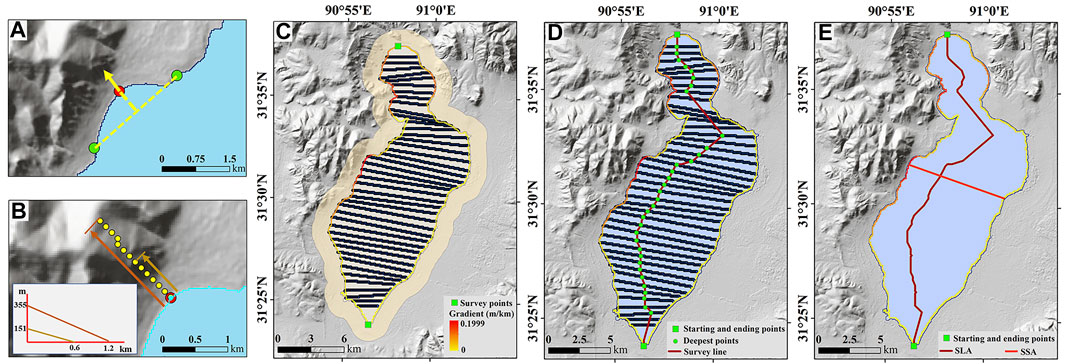
FIGURE 3. Steps for generating the optimized survey lines along the major axis and minor axis. (A) Vertical angle of the center pixel (red point) is calculated using two adjacent points (green points). (B) Gradient calculation using different buffer sizes. (C) Cross sections generation. (D) The predicted deepest points in each cross section were used for creating the optimized survey line along the major axis. (E) The pixel along the lake shoreline with the largest gradient value was selected to develop the optimized survey line along the minor axis.
Both the SAC and SLA are along the lake’s major axis, leading to a great deal of survey work, especially for the long-sharp lake. To improve the practicability of the proposed approach, whether the underwater surveys along the short axis can ensure the estimation accuracy is also investigated by using the SSA strategy. The SSA is easy to generate with a two-step process. The first step is to detect the lake-shoreline pixel with the highest gradient value. As the underwater topography is a spatial extension of the exposed terrains, the deepest zone of a lake is likely to be close to the lake shoreline with the steepest surrounding landscapes. Hence, the second step generates a perpendicular line to the lake boundary direction. As shown in Figure 3E, the created SSA is much shorter than SLA. Meanwhile, its straight direction is another advantage in practical application.
Both lake-bottom elevation and the corresponding lake area are essential for estimating the lake volume. Unfortunately, the lake-bottom site is hard to measure with limited underwater surveys. It is predicted using the constructed E-A relationship (Figures 4A,B) and the measured “maximum” lake depth (transferred to lake-bottom elevation). However, the differences in lake geometry and topography between water-fluctuated and underwater regions may cause the uncertainty of lake area prediction, even leading to a negative value. This study used an alternative method by referring to the ratio between survey length within the bottom zone and the total length. As shown in Figure 4C, after detecting the point with the maximum depth, all the points with a relative elevation of fewer than 1 m are labeled as the lake bottom. The ratio of the lake-bottom area is assumed to be approximately equal to the percentage of lake-bottom length. Hence, the lake bottom area can be calculated by multiplying the lake surface area and the bottom length ratio.
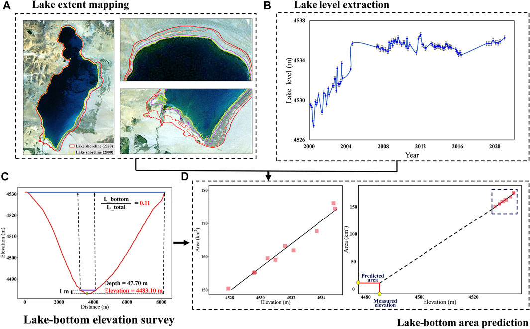
FIGURE 4. Workflow for predicting the lake-bottom area (A,B) Lake extent mapping and lake level extraction are conducted to pair up E-A relationship. (C) Vertical profile along the survey line was generated as the lowest elevation was selected as the lake-bottom elevation. (D) Lake-bottom area was predicted by using the measured elevation and the E-A relationship.
After obtaining the lake-bottom area and elevation (Figure 4D), the total lake volume can be estimated by calculating the difference value between the bottom zone and the referenced lake extent. Although the direct calculation is not infeasible due to the lack of lake bathymetry, we adopted the solid geometry method assuming that a lake can be simplified as a frustum (Abileah and Vignudelli, 2011). In this case, the volume between two conical surfaces can be calculated using the following equation: (eq. 1):
where V is the lake volume, Href and Hbottom are the water levels in the referenced time and that of bottom area, respectively, and Aref and Abottom represent the lake areas. The accuracy of the adopted hypsometric analysis has been proven by the comparation with in-situ measurement of lake volume change for Nam Co. (Zhang et al., 2011).
As most lakes on the TP experienced a rapid expansion trend in the 21st century, the newly inundated area can be captured by the SRTM DEM collected in February 2000. Hence, the total lake volume in 2000 is regarded as the benchmark data which remains to be estimated in this study.
There are strong linear relations between lake levels and area changes, with R2 values larger than 0.9 for all study lakes (Figure 5). To obtain the lake-bottom area by employing the constructed E-A relationship, a constraint value of lake depth is necessary based on the underwater measurements with the optimized survey lines. Both SLC and SLA are along the lake’s major axis (Figure 6). SLA is more zigzagged and longer than the SLC because its generation considers the influence of surrounding topography. The depth bias is used to evaluate whether the survey line had gone through the deepest zone. Table 2 indicates that the SLC is generally acceptable, with a bias of less than 10% in all cases except the Bangda Co. The SLA further reduces the depth bias in the case of Aksai Chin Lake, Bangda Co, Kusai Lake, and Pung Co. However, SLA even achieves a larger bias in another four lakes (Tangra Yumco, Manasarovar Lake, and Zharinam Co), although more complex and longer underwater surveys need to be conducted. There is no doubt that the SSA exhibits a huge advantage in reducing the survey work. For example, the length of the SSA in Kusai Lake is only 4.14 km, reducing about 90% of survey work compared with those created by SLA or SLC. Nevertheless, the simplified survey line is challenging in detecting the deepest area. Fortunately, most lakes agree with the assumption that the deepest underwater area is close to the steepest lake shoreline, except for Kusai Lake and Zharinam Co Particularly in the case of Kusai Lake, the water depth estimated based on SSA has an underestimation bias of 28.33%.
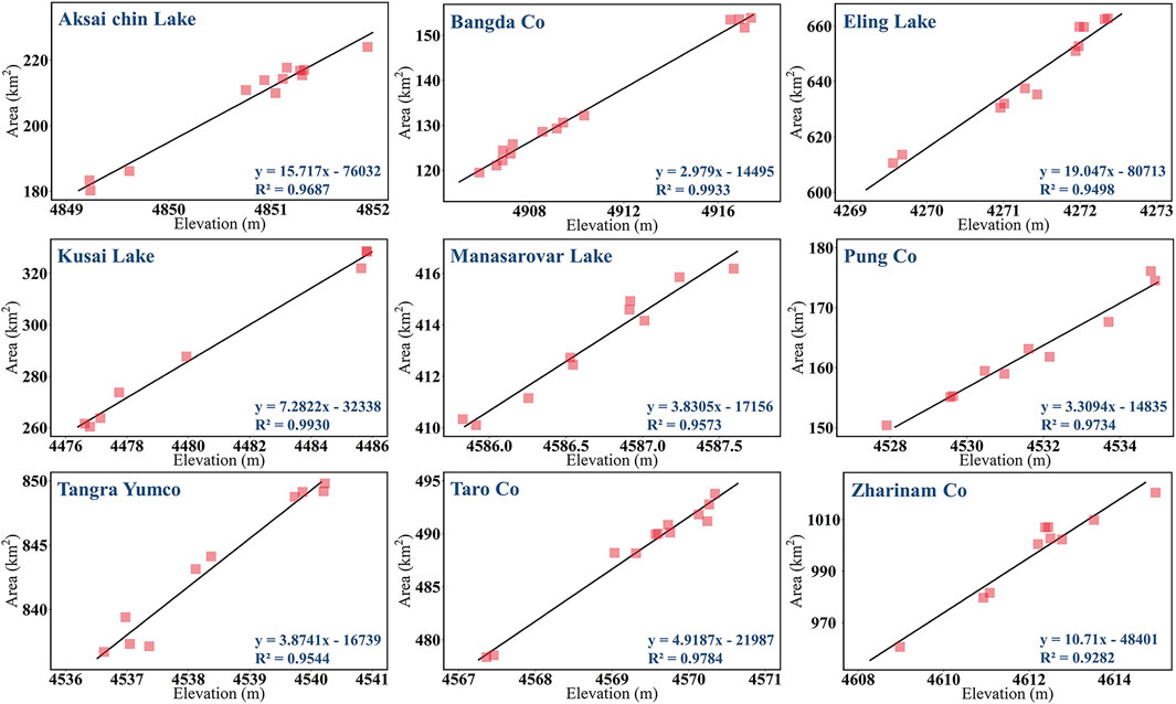
FIGURE 5. E-A relationship of nine selected lakes.
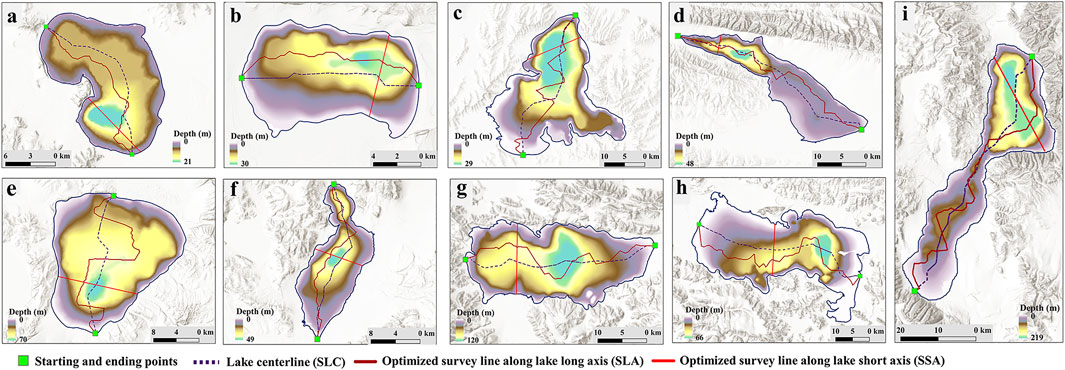
FIGURE 6. The generated survey line using three different strategies. The lakes are in order as follows: Aksai Chin Lake, Bangda Co, Eling Lake, Kusai Lake, Manasarovar Lake, Pung Co, Taro Co, Zharinam Co, and Tangra Yumco.
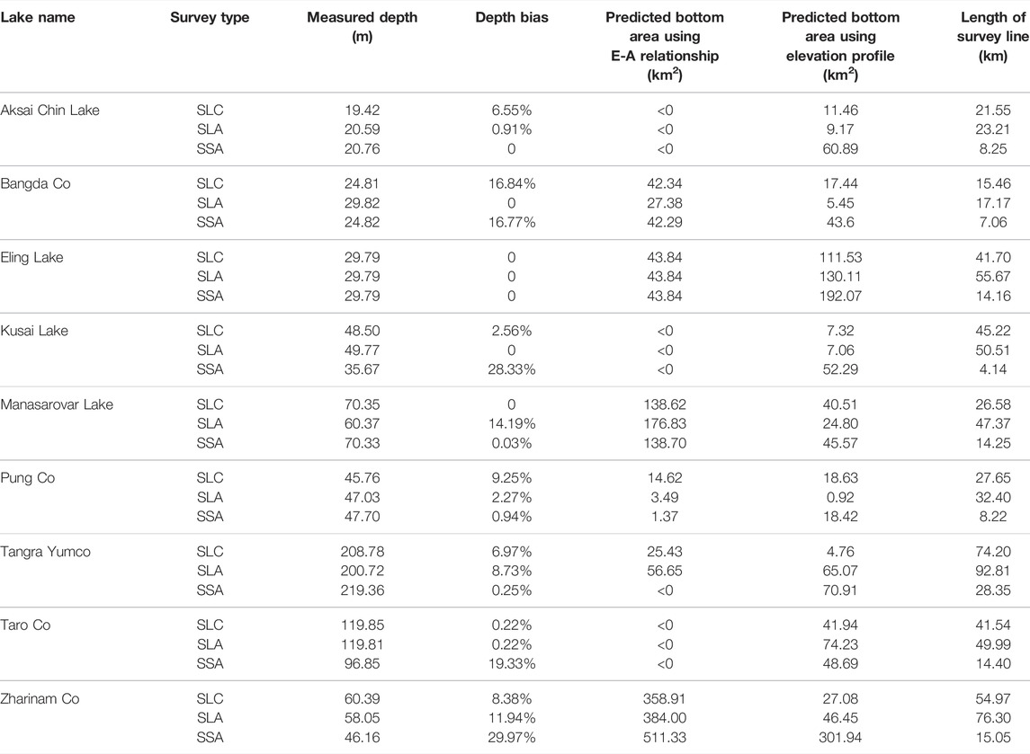
TABLE 2. Measured lake depth and predicted lake bottom area under different survey strategies.
After deciding the lake bottom elevation, the corresponding lake area was calculated based on the constructed E-A relationship. The lake-bottom areas were predicted based on the assumption that the E-A relationship within the water-fluctuating region could be extended to the permanently inundated area. It should be noted that the predicted lake area cannot be accepted if the value is less than zero. In this case, the expected bottom area was calculated using the lake surface area and lake-bottom ratio. As shown in Table 2, such an alternative solution was used in the case of Aksai Chin Lake, Tangra Yumco, Kusai Lake, and Taro Co.
In this study, we calculated the lake volume of each lake based on the circa-2000 lake map and the corresponding lake level. The comparison of the predicted volumes among three different survey strategies is listed in Table 3. The bias of lake volume between referenced data derived from the lake bathymetry and the estimated value by using the proposed method was used for accuracy assessment. Generally, the bias of the lake volume in most cases is less than 30%. The mean bias values of SLC, SLA, and SSA are 22.97, %, 23.83%, and 15.99%. Although the SSA is restricted in survey length, its performance accuracy is even higher than the other two survey strategies. SSA achieved the lowest bias in the case of Aksai Chin Lake, Bangda Co, Pung Co, Tangra Yumco, and Zharinam Co. This strategy balanced well between efficiency and accuracy and is strongly recommended for determining the lake-bottom elevation in the proposed method. It is worth noting the volume bias is negative for most of the lakes, suggesting that the proposed method trends to achieve an overall underestimation of lake volume. This phenomenon should not be entirely ascribed to the missing of the deepest zone. For example, all the three strategies of the water-depth survey line can search the deepest elevation of Eling Lake. However, its water volume estimate is still highly underestimated. It is inferred that the unconformity between the variation of lake geometry and the simplified processing may induce uncertainties in lake volume estimation. Besides estimating the lake volume in 2000, the elevation-volume (E-V) relationship was also constructed by using ten equal interval elevations from the lake bottom to lake level in 2000 (Figure 7). The constructed E-V relationship can estimate the lake volume when the lake level is below that of 2000.
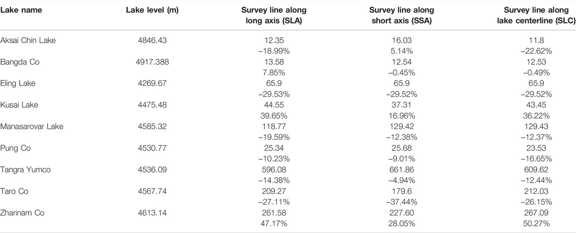
TABLE 3. The predicted lake volumes (108 m3) and the volume bias under different survey strategies.
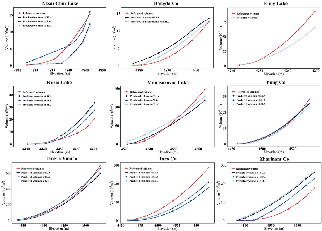
FIGURE 7. Comparations of E-V relationships between the predicted results and the reference data.
This study does not attempt to extrapolate the E-V curve to the lake level above the benchmark value obtained in 2000. As the SRTM DEM can capture the newly exposed region, the gained lake volume since 2000 can be calculated directly. After adding the benchmark volume in 2000, we can estimate the lake volume in any period with a higher lake level. Beneficial from the available topography in the newly flooded region, the bias of the estimated volume is likely to decline when a higher lake level is adopted. For example, the estimated lake volume of Zharinam Co based on the SSA strategy was obviously overestimated in 2000, with a volume bias of 28.05%. After experiencing a dramatic lake expansion, the estimated volume increased from 22.76 Gt to 27.98 Gt. Meanwhile, the bias of the estimated volume dropped to 22.77%.
To facilitate potential applications of our proposed method, we here discuss how the lake volume estimation could be influenced, including the buffer size in lakeside slope calculation and the simplification of lake morphology.
Buffer size determines the width of the exposed terrains around a lake used for calculating the shoreline gradient value. The variation of the estimated gradient value will further lead to different survey routes. This study suggests the default buffer size of 600 m based on previous studies (Liu and Song, 2022). We also investigate the influences of the buffer selection on the survey line generation. As shown in Figure 8, four buffer sizes ranging from 300 to 1200 m were used to generate the survey routes by taking Pung Co and Manasarovar Lake as examples. The generated SLA becomes more zigzag as the increase of buffer size. It can be explained by the potentially greater difference in topographic relief between two sides when a large buffer size was used. The varying buffer size could also lead to the change of detected SSA. It should be noted that only the deepest value along the survey routes was further used for lake volume calculation. In this case, the variation of survey routes has little impact on the final results, except for the generated SSA when the buffer size was set to 1200.
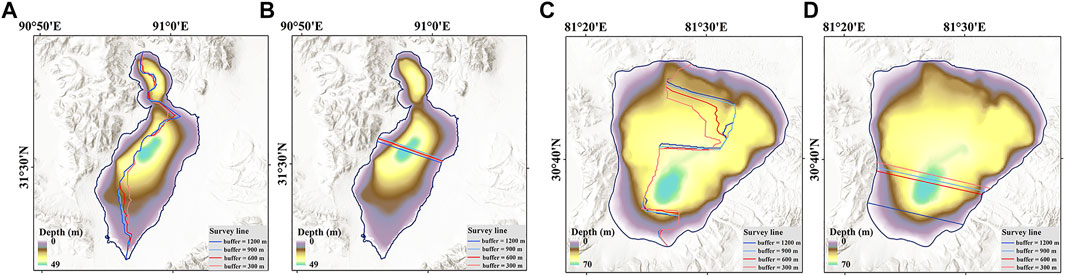
FIGURE 8. The generated survey lines (in long and short axis) using four different buffer sizes (A,B) Pung Co and (C,D) Manasarovar Lake.
Another factor that may cause the uncertainty of the proposed method is the simplified processing of the lake’s geometric shape. In this study, the underlying assumption of the E-A relationship application in estimating the lake-bottom area is that the lake was approximated as a cone. However, the spatial heterogeneity of the lake geometry between the water-fluctuating region zone and permanently standing water region may cause biased predictions of the lake-bottom area. We also noticed its potential influences as the negative lake area appeared in a few cases. Therefore, an alternative method was adopted by calculating the ratio of bottom area to lake surface area using the measured elevation profile. Such similar simplification may also bring uncertainties in lake total volume calculation. As the lake bathymetry mapping is not the target of this study, the water volume estimation in which a cone approximation provides the mathematics method. However, the reported studies indicated that the lake waterbody could be approximated by various geometric shapes such as box, triangular prism, ellipsoid, and the cone (Khazaei et al., 2022). The unified treatment of a cone shape has improved the efficiency, while the oversimplification restricted its performance for effective representation in some cases.
To better understand the characteristics of the proposed method, a comparison with the existing approaches was further conducted (Table 4). HydroLAKES provided the estimated lake volume globally by utilizing the geo-statistical model based on the connection between lake mean depth and lake surrounding terrains (Messager et al., 2016). In this study, Zharinam Co and Tangra Yumco were excluded from the comparison as their volumes were collected from literature records rather than the modeling estimates according to the data specification in HydroLAKES. In comparison, the predicted water volumes for the other seven lakes in HydroLAKES have larger errors than the proposed method. Without any constraint from underwater surveys, the HydroLAKES volume values of Kusai Lake, Pung Co, and Taro Co’s are biased greater than 30%. For Longmu Lake, a case not involved in this study, the estimated volume (1.03 Gt) is even less than half of the referenced volume (2.52 Gt).
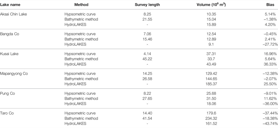
TABLE 4. Comparation between the proposed hypsometric curve method and the results provided by Bathymetric method and HydroLAKES.
A comparison was also conducted between this study and the our pervious study, in which the lake bathymetry was constructed based on the machine-learning method and the limited underwater surveys along the lake centerline (Liu and Song, 2022). Generally, the performance of the lake volume based on the constructed bathymetry is better, with the volume bias less than 20% for all the selected lakes. Specifically, eight of the selected lakes achieved a higher volume bias based on the proposed method, except for Bangda Co. However, sufficient underwater surveys are not feasible for all the lakes on the TP due to the limitation of time cost and weather conditions. The advantage of the proposed method is its minimized cost of underwater surveys. The optimized survey line along the short axis is likely to achieve the deepest underwater elevation at a minimal cost. Hence, this method could effectively complement the large-scale lake investigation in the TP or similar harsh environments.
In order to overcome the challenges in lake volume estimation over the TP, this study aims to propose an efficient method by integrating the remote sensing data and limited underwater surveys. Lake bathymetry, the base data for a commonly-used method for lake volume estimation, is no longer a prerequisite in this method. Instead, this study estimates the lake volume by coupling the lake hypsometric curve and bottom elevation based on the minimal field survey of water depths. The key issue of this method is how to detect the lake-bottom zone without full-coverage measurements. Three survey route strategies were designed, including the lake centerline and the optimized survey lines along the lake’s long axis and short axis. The performances of the proposed methods were demonstrated on nine typical lakes over the TP. Generally, the proposed method with three survey strategies can produce acceptable estimates of lake water volume. The mean value of the estimated bias is approximately 20% for the three strategies. An optimized survey line along the lake short axis is highly recommended because its survey work is much less than the other two strategies, with a good balance between efficiency and accuracy.
This study provides a practical approach for simplifying the lake volume estimation and has the potential to narrow the knowledge gap in quantifying the lake volume of the TP. Although the uncertainties of this approach in some specific lakes cannot be ignored, it is still a necessary supplement for the ongoing project of lake bathymetry measurement across the TP. In addition, this approach is promising to be applied in other remote and data-scarce areas for investigating the lake volume with limited filed work. A better representation of the lake physical characteristics will provide essential information for understanding hydrological fluxes and managing water resources.
Landsat-7 ETM+ and Landsat-8 OLI images are stored in Google Earth Engine cloud computing platform (https://earthengine.google.com/). MERIT DEM is available at http://hy-dro.iis.u-tokyo.ac.jp/yamadai/MERIT_DEM/. The time series of the water level are obtained from online databases (HYDROWEB: http://hydroweb.theia-land.fr/; DAHITI: http://dahiti.dgfi.tum.de/en/). Further inquiries can be directed to the corresponding author.
CS and KL designed the study. PZ and SL provided data. KL and CF analyzed the data. KL and CS led the writing of the manuscript. All authors contributed to the article and approved the submitted version.
This study was supported by the Second Tibetan Plateau Scientific Expedition and Research (STEP) (Grant No.2019QZKK0202), and the National Natural Science Foundation of China (Grant Nos. 42171421, 41971403, and 41930102).
The authors declare that the research was conducted in the absence of any commercial or financial relationships that could be construed as a potential conflict of interest.
All claims expressed in this article are solely those of the authors and do not necessarily represent those of their affiliated organizations, or those of the publisher, the editors and the reviewers. Any product that may be evaluated in this article, or claim that may be made by its manufacturer, is not guaranteed or endorsed by the publisher.
We are grateful to the satellite data providers: USGS for Landsat, NSIDC for ICESat/ICESat-2, LEGOS for Hydroweb, Yamazaki Lab for MERIT DEM. We also grateful to the scientific editor and the reviewers for their valuable comments on the manuscript.
Abileah, R., and Vignudelli, S. (2011). “A Completely Remote Sensing Approach to Monitoring Reservoirs Water Volume,” in Fifteenth International Water Technology Conference, IWTC 15, Alexandria, Egypt, 29 May, 2011, 59–72.
Armon, M., Dente, E., Shmilovitz, Y., Mushkin, A., Cohen, T. J., Morin, E., et al. (2020). Determining Bathymetry of Shallow and Ephemeral Desert Lakes Using Satellite Imagery and Altimetry. Geophys. Res. Lett. 47, 1–9. doi:10.1029/2020GL087367
Bandini, F., Olesen, D., Jakobsen, J., Kittel, C. M. M., Wang, S., Garcia, M., et al. (2018). Technical Note: Bathymetry Observations of Inland Water Bodies Using a Tethered Single-Beam Sonar Controlled by an Unmanned Aerial Vehicle. Hydrol. Earth Syst. Sci. 22, 4165–4181. doi:10.5194/hess-22-4165-2018
Busker, T., de Roo, A., Gelati, E., Schwatke, C., Adamovic, M., Bisselink, B., et al. (2019). A Global Lake and Reservoir Volume Analysis Using a Surface Water Dataset and Satellite Altimetry. Hydrol. Earth Syst. Sci. 23, 669–690. doi:10.5194/hess-23-669-2019
Cael, B. B., Heathcote, A. J., and Seekell, D. A. (2017). The Volume and Mean Depth of Earth's Lakes. Geophys. Res. Lett. 44, 209–218. doi:10.1002/2016GL071378
Chen, F., Zhang, J., Liu, J., Cao, X., Hou, J., Zhu, L., et al. (2020). Climate Change, Vegetation History, and Landscape Responses on the Tibetan Plateau during the Holocene: A Comprehensive Review. Quat. Sci. Rev. 243, 106444. doi:10.1016/j.quascirev.2020.106444
Cheng, J., Song, C., Liu, K., Fan, C., Ke, L., Chen, T., et al. (2022). Satellite and UAV-Based Remote Sensing for Assessing the Flooding Risk from Tibetan Lake Expansion and Optimizing the Village Relocation Site. Sci. Total Environ. 802, 149928. doi:10.1016/j.scitotenv.2021.149928
Coggins, L. X., and Ghadouani, A. (2019). High-Resolution Bathymetry Mapping of Water Bodies: Development and Implementation. Front. Earth Sci. 7, 1–11. doi:10.3389/feart.2019.00330
Crétaux, J.-F., Arsen, A., Calmant, S., Kouraev, A., Vuglinski, V., Bergé-Nguyen, M., et al. (2011). SOLS: A Lake Database to Monitor in the Near Real Time Water Level and Storage Variations from Remote Sensing Data. Adv. Space Res. 47, 1497–1507. doi:10.1016/j.asr.2011.01.004
Fassoni‐Andrade, A. C., Paiva, R. C. D., and Fleischmann, A. S. (2020). Lake Topography and Active Storage from Satellite Observations of Flood Frequency. Water Resour. Res. 56, 1–18. doi:10.1029/2019WR026362
Getirana, A., Jung, H. C., and Tseng, K.-H. (2018). Deriving Three Dimensional Reservoir Bathymetry from Multi-Satellite Datasets. Remote Sens. Environ. 217, 366–374. doi:10.1016/j.rse.2018.08.030
Heathcote, A. J., del Giorgio, P. A., and Prairie, Y. T. (2015). Predicting Bathymetric Features of Lakes from the Topography of Their Surrounding Landscape. Can. J. Fish. Aquat. Sci. 72, 643–650. doi:10.1139/cjfas-2014-0392
Hollister, J. W., Milstead, W. B., and Urrutia, M. A. (2011). Predicting Maximum Lake Depth from Surrounding Topography. PLoS One 6, e25764–6. doi:10.1371/journal.pone.0025764
Immerzeel, W. W., and Bierkens, M. F. P. (2012). Asia's Water Balance. Nat. Geosci. 5, 841–842. doi:10.1038/ngeo1643
Jia, W., and Liu, X. (2019). Decadal- to Centennial-Scale Climate Changes over the Last 2000 Yr Recorded from Varved Sediments of Lake Kusai, Northern Qinghai-Tibetan Plateau. Quat. Res. 92, 340–351. doi:10.1017/qua.2019.19
Khazaei, B., Read, L. K., Casali, M., Sampson, K. M., and Yates, D. N. (2022). GLOBathy, the Global Lakes Bathymetry Dataset. Sci. Data 9, 1–10. doi:10.1038/s41597-022-01132-9
Lei, Y., Yao, T., Bird, B. W., Yang, K., Zhai, J., and Sheng, Y. (2013). Coherent Lake Growth on the Central Tibetan Plateau since the 1970s: Characterization and Attribution. J. Hydrology 483, 61–67. doi:10.1016/j.jhydrol.2013.01.003
Li, X., Long, D., Huang, Q., Han, P., Zhao, F., and Wada, Y. (2019a). High-temporal-resolution Water Level and Storage Change Data Sets for Lakes on the Tibetan Plateau during 2000-2017 Using Multiple Altimetric Missions and Landsat-Derived Lake Shoreline Positions. Earth Syst. Sci. Data 11, 1603–1627. doi:10.5194/essd-11-1603-2019
Li, Y., Gao, H., Allen, G. H., and Zhang, Z. (2021). Constructing Reservoir Area-Volume-Elevation Curve from TanDEM-X DEM Data. IEEE J. Sel. Top. Appl. Earth Obs. Remote Sens. 14, 2249–2257. doi:10.1109/JSTARS.2021.3051103
Li, Y., Gao, H., Jasinski, M. F., Zhang, S., and Stoll, J. D. (2019b). Deriving High-Resolution Reservoir Bathymetry from ICESat-2 Prototype Photon-Counting Lidar and Landsat Imagery. IEEE Trans. Geosci. Remote Sens. 57, 7883–7893. doi:10.1109/tgrs.2019.2917012
Li, Y., Gao, H., Zhao, G., and Tseng, K.-H. (2020). A High-Resolution Bathymetry Dataset for Global Reservoirs Using Multi-Source Satellite Imagery and Altimetry. Remote Sens. Environ. 244, 111831. doi:10.1016/j.rse.2020.111831
Liu, C., Zhu, L., Wang, J., Ju, J., Ma, Q., Qiao, B., et al. (2021a). In-situ Water Quality Investigation of the Lakes on the Tibetan Plateau. Sci. Bull. 66, 1727–1730. doi:10.1016/j.scib.2021.04.024
Liu, K., Ke, L., Wang, J., Jiang, L., Richards, K. S., Sheng, Y., et al. (2021b). Ongoing Drainage Reorganization Driven by Rapid Lake Growths on the Tibetan Plateau. Geophys. Res. Lett. 48, 1–11. doi:10.1029/2021GL095795
Liu, K., Song, C., Ke, L., Jiang, L., Pan, Y., and Ma, R. (2019). Global Open-Access DEM Performances in Earth's Most Rugged Region High Mountain Asia: A Multi-Level Assessment. Geomorphology 338, 16–26. doi:10.1016/j.geomorph.2019.04.012
Liu, K., and Song, C. (2022). Modeling Lake Bathymetry and Water Storage from DEM Data Constrained by Limited Underwater Surveys. J. Hydrology 604, 127260. doi:10.1016/j.jhydrol.2021.127260
Luo, S., Song, C., Zhan, P., Liu, K., Chen, T., Li, W., et al. (2021). Refined Estimation of Lake Water Level and Storage Changes on the Tibetan Plateau from ICESat/ICESat-2. Catena 200, 105177. doi:10.1016/j.catena.2021.105177
Ma, Q., Zhu, L., Lü, X., Guo, Y., Ju, J., Wang, J., et al. (2014). Pollen-inferred Holocene Vegetation and Climate Histories in Taro Co, Southwestern Tibetan Plateau. Chin. Sci. Bull. 59, 4101–4114. doi:10.1007/s11434-014-0505-1
Messager, M. L., Lehner, B., Grill, G., Nedeva, I., and Schmitt, O. (2016). Estimating the Volume and Age of Water Stored in Global Lakes Using a Geo-Statistical Approach. Nat. Commun. 7, 1–11. doi:10.1038/ncomms13603
Pekel, J.-F., Cottam, A., Gorelick, N., and Belward, A. S. (2016). High-resolution Mapping of Global Surface Water and its Long-Term Changes. Nature 540, 418–422. doi:10.1038/nature20584
Qiao, B., Zhu, L., Wang, J., Ju, J., Ma, Q., Huang, L., et al. (2019a). Estimation of Lake Water Storage and Changes Based on Bathymetric Data and Altimetry Data and the Association with Climate Change in the Central Tibetan Plateau. J. Hydrology 578, 124052. doi:10.1016/j.jhydrol.2019.124052
Qiao, B., Zhu, L., Wang, J., Ju, J., Ma, Q., and Liu, C. (2017). Estimation of Lakes Water Storage and Their Changes on the Northwestern Tibetan Plateau Based on Bathymetric and Landsat Data and Driving Force Analyses. Quat. Int. 454, 56–67. doi:10.1016/j.quaint.2017.08.005
Qiao, B., Zhu, L., and Yang, R. (2019b). Temporal-spatial Differences in Lake Water Storage Changes and Their Links to Climate Change throughout the Tibetan Plateau. Remote Sens. Environ. 222, 232–243. doi:10.1016/j.rse.2018.12.037
Saylam, K., Brown, R. A., and Hupp, J. R. (2017). Assessment of Depth and Turbidity with Airborne Lidar Bathymetry and Multiband Satellite Imagery in Shallow Water Bodies of the Alaskan North Slope. Int. J. Appl. Earth Observation Geoinformation 58, 191–200. doi:10.1016/j.jag.2017.02.012
Sheng, Y., Song, C., Wang, J., Lyons, E. A., Knox, B. R., Cox, J. S., et al. (2016). Representative Lake Water Extent Mapping at Continental Scales Using Multi-Temporal Landsat-8 Imagery. Remote Sens. Environ. 185, 129–141. doi:10.1016/j.rse.2015.12.041
Song, C., Huang, B., and Ke, L. (2013). Modeling and Analysis of Lake Water Storage Changes on the Tibetan Plateau Using Multi-Mission Satellite Data. Remote Sens. Environ. 135, 25–35. doi:10.1016/j.rse.2013.03.013
Song, C., Ke, L., Pan, H., Zhan, S., Liu, K., and Ma, R. (2018). Long-term Surface Water Changes and Driving Cause in Xiong'an, China: from Dense Landsat Time Series Images and Synthetic Analysis. Sci. Bull. 63, 708–716. doi:10.1016/j.scib.2018.05.002
Verpoorter, C., Kutser, T., Seekell, D. A., and Tranvik, L. J. (2014). A Global Inventory of Lakes Based on High-Resolution Satellite Imagery. Geophys. Res. Lett. 41, 6396–6402. doi:10.1002/2014GL060641
Wang, J., Peng, P., Ma, Q., and Zhu, L. (2010). Modem Limnological Features of Tangra Yumco and Zhari Namco, Tibetan Plateau. J. Lake Sci. 22 (4), 629–632. (In Chinese with English abstract)
Wang, J., Peng, P., Ma, Q., and Zhu, L. (2013). Investigation of Water Depth, Water Quality and Modern Sedimentation Rate in MapamYumco and La’ang Co, Tibet. J. Lake Sci. 25 (4), 609–616. (In Chinese with English abstract)
Woolway, R. I., Kraemer, B. M., Lenters, J. D., Merchant, C. J., O’Reilly, C. M., and Sharma, S. (2020). Global Lake Responses to Climate Change. Nat. Rev. Earth Environ. 1, 388–403. doi:10.1038/s43017-020-0067-5
Xu, N., Ma, Y., Yang, J., Wang, X. H., Wang, Y., and Xu, R. (2022). Deriving Tidal Flat Topography Using ICESat‐2 Laser Altimetry and Sentinel‐2 Imagery. Geophys. Res. Lett. 49, 1–10. doi:10.1029/2021gl096813
Yamazaki, D., Ikeshima, D., Tawatari, R., Yamaguchi, T., O'Loughlin, F., Neal, J. C., et al. (2017). A High-Accuracy Map of Global Terrain Elevations. Geophys. Res. Lett. 44, 5844–5853. doi:10.1002/2017GL072874
Yang, K., Lu, H., Yue, S., Zhang, G., Lei, Y., La, Z., et al. (2018). Quantifying Recent Precipitation Change and Predicting Lake Expansion in the Inner Tibetan Plateau. Clim. Change 147, 149–163. doi:10.1007/s10584-017-2127-5
Yao, F., Wang, J., Yang, K., Wang, C., Walter, B. A., and Crétaux, J.-F. (2018). Lake Storage Variation on the Endorheic Tibetan Plateau and its Attribution to Climate Change since the New Millennium. Environ. Res. Lett. 13, 064011. doi:10.1088/1748-9326/aab5d3
Yigzaw, W., Li, H. Y., Demissie, Y., Hejazi, M. I., Leung, L. R., Voisin, N., et al. (2018). A New Global Storage‐Area‐Depth Data Set for Modeling Reservoirs in Land Surface and Earth System Models. Water Resour. Res. 54 (10), 372–410. doi:10.1029/2017WR022040
Zhang, B., Wu, Y., Zhu, L., Wang, J., Li, J., and Chen, D. (2011). Estimation and Trend Detection of Water Storage at Nam Co Lake, Central Tibetan Plateau. J. Hydrology 405, 161–170. doi:10.1016/j.jhydrol.2011.05.018
Zhang, G., Ran, Y., Wan, W., Luo, W., Chen, W., Xu, F., et al. (2021a). 100 Years of Lake Evolution over the Qinghai-Tibet Plateau. Earth Syst. Sci. Data 13, 3951–3966. doi:10.5194/essd-13-3951-2021
Zhang, G., Yao, T., Xie, H., Yang, K., Zhu, L., Shum, C. K., et al. (2020). Response of Tibetan Plateau Lakes to Climate Change: Trends, Patterns, and Mechanisms. Earth-Science Rev. 208, 103269. doi:10.1016/j.earscirev.2020.103269
Keywords: lake volume, Tibetan plateau (TP), hypsometric curve, water-depth survey, remote sensing
Citation: Liu K, Song C, Zhan P, Luo S and Fan C (2022) A Low-Cost Approach for Lake Volume Estimation on the Tibetan Plateau: Coupling the Lake Hypsometric Curve and Bottom Elevation. Front. Earth Sci. 10:925944. doi: 10.3389/feart.2022.925944
Received: 22 April 2022; Accepted: 15 June 2022;
Published: 13 July 2022.
Edited by:
Frédéric Frappart, INRAE Nouvelle-Aquitaine Bordeaux, FranceCopyright © 2022 Liu, Song, Zhan, Luo and Fan. This is an open-access article distributed under the terms of the Creative Commons Attribution License (CC BY). The use, distribution or reproduction in other forums is permitted, provided the original author(s) and the copyright owner(s) are credited and that the original publication in this journal is cited, in accordance with accepted academic practice. No use, distribution or reproduction is permitted which does not comply with these terms.
*Correspondence: Chunqiao Song, Y3Fzb25nQG5pZ2xhcy5hYy5jbg==
Disclaimer: All claims expressed in this article are solely those of the authors and do not necessarily represent those of their affiliated organizations, or those of the publisher, the editors and the reviewers. Any product that may be evaluated in this article or claim that may be made by its manufacturer is not guaranteed or endorsed by the publisher.
Research integrity at Frontiers
Learn more about the work of our research integrity team to safeguard the quality of each article we publish.