 Guo Yu
 Lei Bu
 Chengfeng Wang1
94% of researchers rate our articles as excellent or good
Learn more about the work of our research integrity team to safeguard the quality of each article we publish.
Find out more
ORIGINAL RESEARCH article
Front. Earth Sci., 25 July 2022
Sec. Geohazards and Georisks
Volume 10 - 2022 | https://doi.org/10.3389/feart.2022.923620
This article is part of the Research TopicRock Landslide Risk Assessment, Stability Analysis and Monitoring for The Development of Early Warning Systems and Reinforcement MeasuresView all 24 articles
For the limit equilibrium method based on the assumption model of sliding surface normal stress, the more reasonable the assumed sliding surface normal stress model is, the higher the accuracy of the calculation results will be, which is of great significance to improve the theoretical calculation accuracy. Combined with the powerful spatial data analysis ability of Geographic Information Systems (GIS), the expression of the normal stress distribution function of the slip surface is deduced by establishing a GIS-based three-dimensional slope stability analysis model and limit equilibrium equations. By analyzing the composition of the normal stress distribution on the sliding surface, the composition of the normal stress on the sliding surface is obtained, and then the assumed model of the normal stress distribution on the sliding surface is constructed. Finally, the assumed GIS model of the sliding surface normal stress distribution is verified by calculating the proportion. The model overcomes the problem that the stability factor of the slope will cause large errors in the three-dimensional state, and provides a theoretical calculation basis for the establishment of a three-dimensional slope limit equilibrium method based on the assumption of normal stress on the slip surface in GIS.
Limit equilibrium method is a common analysis method to analyze the stability of slope, and after years of development (Zhou and Cheng, 2013; Du et al., 2019; Du et al., 2020; Du et al., 2021), relevant theories currently have been improved and played an important role in the stability analysis method. Scholars have been exploiting the analysis method of 2D slopes into 3D slopes, for example, Hovland (1979), Hungr (1987), Cheng and Yip (2007), Low Wilson (1997). Extended the two-dimensional models of Hovland, Bishop and Janbu into three-dimensional models, but these methods all need to solve the stability factor by assuming the force between bars or columns, and it is difficult to meet the strict calculation of static balance conditions. Later, Bell (1968), Zhu and Lee (2002), Zhu et al. (2004), Zhu et al. (2009), Yang (2004), Zheng and Tham (2010) assumed that the normal stress distribution pattern of the sliding surface is a function containing multiple dimensionless parameters, to find the stability factor. The advantage of this method is that it does not need to assume the stress and distribution between bars or columns, and the obtained stability factor is closer to the true value. However, the normal stress distribution mode assumed in this kind of method cannot truly reflect the normal stress of the slip surface, so the accuracy of the results calculated by this kind of method is not high.
At the same time, in the calculation of slope stability, GIS is more widely used because it has powerful spatial data processing abilities, as well as unique advantages in the processing of three-dimensional data, and the complex mathematical calculations and difficult algorithms encountered in the process can also be well solved in GIS (Zhou et al., 2003; Ayalew and Yamagishi, 2005). In the study of GIS combined with the limit equilibrium method, Xie et al. (2003), Xie et al. (2006a, 2006b). Extended the 2D model of Hovland, Bishop and Janbu to a 3D model based on the advantages of GIS 3D data processing and developed a 3D limit equilibrium analysis software 3DSlope. However, the establishment of the three-dimensional limit equilibrium method based on the assumption of the normal stress of the sliding surface in GIS has not been studied by scholars. The key step of this method is to establish an assumed model of the normal stress distribution of the sliding surface based on GIS. The more reasonable the assumed model is, the smaller the impacts on stability factors closer the results to the actual value.
Regarding the assumed mode of the normal stress distribution on the sliding surface, for a two-dimensional slope, the difference in the influence of different normal stress distributions on the sliding surface on the slope stability factor is about 19%. After the rationality verification of the inter stripe force distribution, the difference can be reduced to within 7%, to meet the needs of engineering. However, the influence range of three-dimensional state will be greatly increased. Therefore, establish a three-dimensional limit equilibrium method based on the normal stress of the sliding surface in GIS, it is necessary to construct a reasonable three-dimensional sliding surface normal stress assumption model based on GIS to ensure the accuracy of calculation results.
In this paper, by introducing GIS and using its spatial data analysis capability, a hypothetical model of the normal stress distribution of a three-dimensional slope sliding surface is constructed based on the grid column units. Based on GIS, a three-dimensional slope stability analysis limit equilibrium model is established, and the limit equilibrium equation for solving the stability factor is deduced according to the limit equilibrium conditions. And then under the assumption of no force, the distribution composition of normal stress on sliding surface based on the grid column units is deduced and analyzed and later a hypothetical model of the normal stress distribution of the three-dimensional symmetrical slope sliding surface based on GIS is constructed. The assumed model not only overcomes the problem of large errors in the slope stability factor in the three-dimensional state, but also provides a theoretical basis for the establishment of a three-dimensional symmetrical slope limit equilibrium method in GIS based on the assumption of sliding surface normal stress.
Generally, slope data is mostly expressed in the form of two-dimensional vector data, such as ground contours, rock formations, groundwater and mechanical parameters. In GIS, these two-dimensional vector data layers can be converted into GIS-based three-dimensional grid column unit structure data layers by using the spatial analysis function. Therefore, all the data related to the slope can come from the GIS data layer. And based on the 3D grid column unit data structure of GIS, the limit equilibrium equation for 3D slope stability analysis can be established.
As shown in Figures 1A,B, a grid column unit ABCDA1B1C1D1 is taken in the three-dimensional slide body. For the entire slide body, the force between columns is the internal force, and the force is 0, so it is not marked in the figure. And the acting forces on the grid column mainly include: the weight of the grid column unit W; the horizontal seismic inertial force kW with k as the earthquake influence coefficient; the external force P on the slope surface; the normal total stress and shear stress on the sliding surface are respectively σ and τ; the pore water pressure u on the sliding surface.
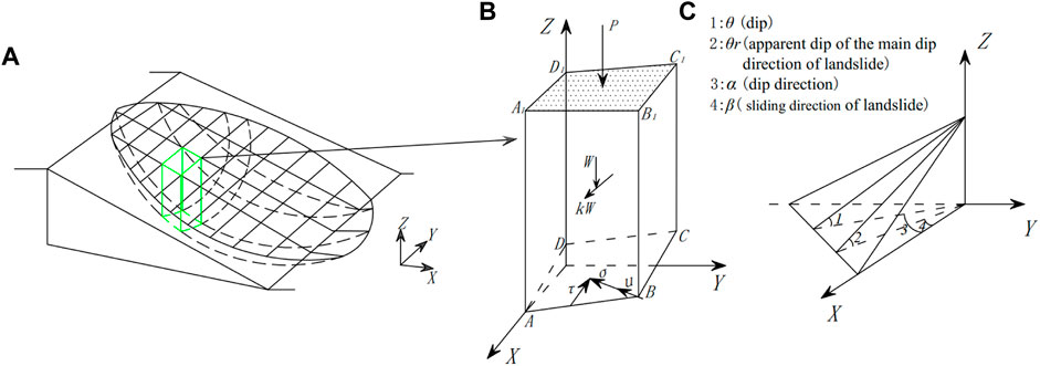
FIGURE 1. Computational modeling and three-dimensional spatial relationship. (A) 3D model of slide body, (B) typical column force analysis, (C) 3D spatial relationship.
Figure 1C shows the spatial relationship of each calculation parameter in the 3D model. On the sliding surface, according to the Mohr-Coulomb criterion:
where c´ and φ′ are the effective cohesion force and the effective internal friction angle, respectively, and FS3D is the three-dimensional stability factor of the slide body.
According to the static force balance of the slide body, for the entire slide body, the force balance equations on the X, Y, and Z axes and a moment balance equation for a rotating axis perpendicular to the sliding direction can be established. The combined force between columns in every axis is 0, then the four equations can be expressed as:
In the formula: J and I are the number of rows and columns of grid units within the slide body range; A is the sliding surface area.
Eqs 1–5 constitute the equilibrium equations for solving the three-dimensional stability factor. Under the assumption of no force, the above 5 equations are simultaneously solved to achieve the normal stress of FS3D and the sliding surface of (J×I) columns, with a total of (J×I+1) unknown numbers, and the number of unknowns is more than the that of equations, hence the equations cannot be solved. If the distribution of the normal stress σ on the sliding surface can be known, it can be solved.
For a single grid column unit, the forces between the columns cannot cancel each other out. Figure 2 is a schematic diagram of the force of a single column. The forces between the columns are horizontal tangential forces T and T+△T on the left and right sides of the column, vertical tangential forces R and R+△R normal Forces F and F+△F; horizontal tangential forces E and E+△E on the front and rear sides, vertical tangential forces V and V+△V, and normal forces H and H+△H. Under the assumption of no force, according to the static balance conditions of a single column, the force balance equation on the X, Y, and Z axes can be obtained as:
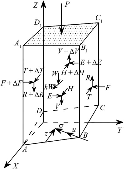
FIGURE 2. Force analysis of a single column.
By eliminating τ from Eqs 6–8, the normal stress distribution function of the sliding surface can be obtained as:
It can be seen from Eq 9 that the distribution of the normal stress on the sliding surface can be divided into two parts, one of which is contributed by the self-weight W of the slide body and the external force P, and the other is contributed by the force between the columns, which can be denoted as σ1 and σ2 respectively. So, formula (9) can be simplified as:
where
If the sliding surface is known, all the parameters in Eq. 11 are known, so σ1 belongs to a known function; however, because the distribution of the force between the columns cannot be accurately obtained, σ2 belongs to an unknown function. At present, in most limit equilibrium analysis methods, certain conditions are generally assumed to solve the stability factor. For example, the Swedish strip method assumes that there is no interaction force between the blocks, the simplified Bishop method assumes that the force between the strips is only horizontal, the simplified Janbu method ignores the shear force between the bars, and the simplified Spencer method assumes that the inclination of the force between bars is a constant.
In order to study the contribution of σ1 and σ2 to the normal stress of the sliding surface, the distribution of σ1 and σ2 is calculated by a calculation example, so that the contribution of each component to the normal stress distribution can be obtained through the actual calculation data. The symmetric slope calculation example is shown in Figure 3 and this calculation example does not consider the influence of earthquake, and the size of the grid unit based on GIS is 0.5 m × 0.5 m.
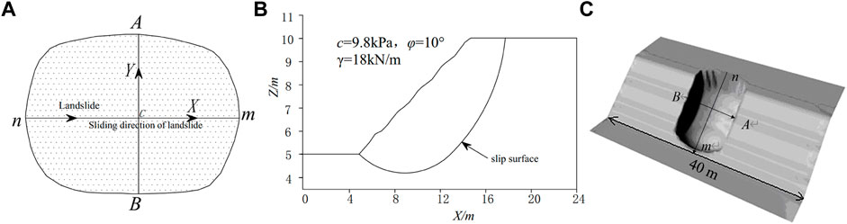
FIGURE 3. Plane and cross-section of slope. (A) plane of slope, (B) cross-section of slope, (C) the DEM model of slope surface.
For this example, the 3D slope stability analysis extension module 3DSlope, which is developed by this research team based on GIS, is used, and two methods, the extended Bishop method and the extended Janbu method based on GIS are applied. The normal stress σ of the sliding surface, as well as the sum of the two component σ1 and σ2 are calculated. A cross-section is drawn along the sliding direction nm of the slide body and perpendicular to the sliding direction AB of the slide body respectively, and then the results of σ、σ1 and σ2 are recorded in Figure 4. Due to the limitation of the three-dimensional effect, only the curves on nm and AB are shown here.
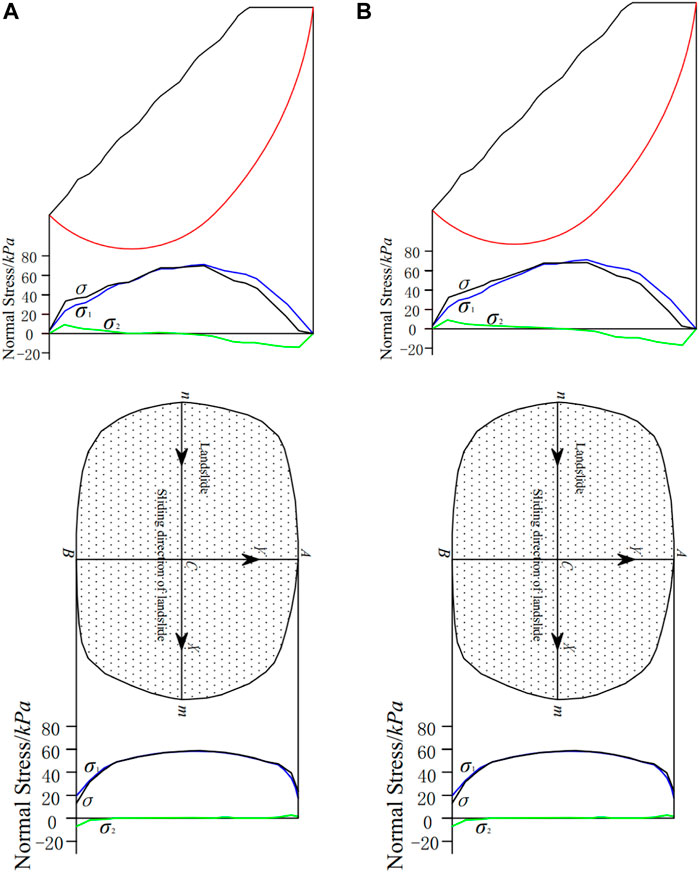
FIGURE 4. Normal stress distributions of slip surface with different calculations. (A) the Bishop method based on GIS (Along the sliding direction of the slide body) and (Perpendicular to the direction of the slide body); (B) the Janbu method based on GIS (Along the sliding direction of the slide body) and (Perpendicular to the direction of the slide body).
It can be concluded from Figure 4: (1) In the composition of the normal stress σ distribution of the sliding surface, the self-weight of the slide body and the external force (σ1) make a large contribution to the normal stress of the sliding surface, while the force between the columns (σ2) contributes very little to the normal stress of the sliding surface; (2) The normal stress of sliding surface σ、σ1 and σ2 are continuous and approximately smooth curves.
It can be concluded from above that: (1) For the sliding direction along the slide body, since the normal stress of the sliding surface accounts for a small proportion and is a continuous and approximately smooth curve, an appropriate function pair can be used for approximation fitting; (2) For the direction perpendicular to the sliding direction of the slide body, the normal stress distribution on the sliding surface is approximated and fitted by a parabola symmetrical along the sliding direction of the slide body.
If the sliding surface is known, in the distribution function of the normal stress σ of the sliding surface, σ1 belongs to a known function, σ2 belongs to an unknown function because the force between the columns is difficult to calculate, hence in order to make Eqs 1–5 have solutions, it is necessary to construct the distribution function σ(x, y) in the normal stress of the sliding surface.
Figure 5 shows the assumed model of the normal stress on the sliding surface. The center of the slide body is C, nm is the long axis direction, FR is the short axis direction, n and m are the peak and the lowest point of the slide body respectively, and the X-axis direction is along the sliding surface with the Y-axis direction perpendicular to the sliding direction. Also, AA and BB represent the two-dimension features of the slide body respectively, and at 1/3 and 2/3 of the X-axis, take two points, m1、m2, respectively, there are:
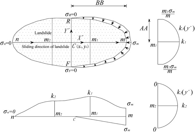
FIGURE 5. Normal stress assumption on the slip surface.
For the cross-section nm along the sliding direction of the slide body, it is obtained through the research in this paper that since σ2(x) occupies a small proportion in the composition of the normal stress σ(x) of the sliding surface, and it is a continuous and approximately smooth curve, it can be considered that σ2(x) can be expressed by an approximation function. Since the proportion of σ2(x) is small, different approximation functions have little effect on the results, so that the normal stress σ(x) of the sliding surface is closer to the distribution in the strict method. Function.
Assuming that the approximation function is β(x), so the distribution function of the normal stress of the sliding surface in the sliding direction of the slide body can be expressed as
In the formula: σ(x) is the distribution function of the normal stress of the sliding surface in the sliding direction of the slide body; σ1(x) is the component of the normal stress of the sliding surface caused by the self-weight of the slide body and the external force in the sliding direction of the slide body, which can be obtained from the formula (11) is determined and belongs to a known function.
For the approximation function β(x), that is, based on the research of Zhu et al., over the section on the X-axis of the sliding direction of the slide body, it is assumed that the normal stress distribution of the sliding surface is a third order Lagrangian polynomial:
where
In the formula: k1 and k2 are the dimensionless calculation parameters; x is the coordinate value of the center of the bottom surface in each grid column unit on the X axis; βm is the corresponding part of the normal stress σ2 of the lowest point m of the slide body; βn is the vertex n of the slide body The corresponding part of the normal stress σ2.
Since the normal stress at the boundary of the upper half of the slide body is small (Leshchinsky, 1990), it is assumed that its normal stress is 0, then βn = 0. And assuming that the normal stress at the boundary of the lower half of the slide body is linearly distributed, that is, its normal stress is x
For the cross-section perpendicular to the sliding direction of the slide body, the distribution of the normal stress is approximated and fitted by a parabola symmetrical along the sliding direction of the slide body (that is, along the X axis).
Then the normal stress distribution σb(y) of any cross-section in the lower half of the slide body and the normal stress distribution σa(y) of any section in the upper half of the slide body are expressed as
Considering the boundary conditions, Eqs 21, 22 can be expressed as
After obtaining the normal stress distribution σ(x) along the sliding direction of the slide body and the normal stress distribution σ(y) perpendicular to the sliding direction of the slide body, for the entire sliding surface, the normal stress distribution σ(x,y)of the sliding surface of any grid column unit can be expressed as
In the formula: σb(y) represents the normal stress distribution of the sliding surface in the lower half of the slide body; σa(y) represents the normal stress distribution on the sliding surface of the upper half of the slide body; AAx is the short axis dimension corresponding to the x axis; y is the corresponding coordinate value on the Y axis.
During the example verification, the approximation function shown in Eq 25 is used for the normal stress of the sliding surface, and the Eqs 1–5 and Eq 25 are combined together. The final four equations, after dividing and eliminating the difference, contain four unknowns (FS3D、σ(m)、k1 and k2), and the number of equations is equal to that of unknowns, so the three-dimensional stability factor FS3D can be solved. For the specific calculation process, please refer to the calculation method proposed by this research team (Yu et al., 2019).
The case shown in Figure 3 is used in combination with the proposed method to calculate, together with the GIS-based 3D Hovland method (Xie et al., 2003), 3D modification Hovland method (Xie et al., 2006a), 3D Bishop method (Xie et al., 2006b), 3D Janbu method (Xie et al., 2006b), 3D Spencer method (Low and Wilson, 1997), and 3D M-P method (Chen and Zhu, 2010), proposed. and used for comparative calculation, and the results are shown in Table 1.
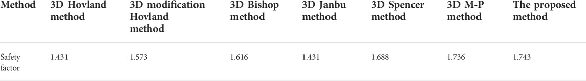
TABLE 1. Calculation results.
From the analysis of the results in Table 1, it can be seen that.
(1) According to the classification method proposed by Deng Dongping, the 3D Hovland method, the 3D modification Hovland method, the 3D Bishop method, and the 3D Janbu method satisfy a smaller amount of equilibrium conditions, so the obtained stability factor is conservative. The method is close to the non-strict method; the Spencer method satisfies the balance conditions of the five forces and is a quasi-strict method; the M-P method satisfies the force and moment balance conditions most, and is a strict method, that is, it is the closest to the true value. And the strict method has the largest result, the quasi-strict method is the second, and the non-strict method is the smallest.
(2) Since the approximation function used by the proposed method is close to the real function, the calculation result of the proposed method is closer to the real value, that is, it is close to the strict method. Seen from the calculation result, the proposed method achieves the biggest data, close to that of the M-P method, as well as that of a strict method, which shows the rationality of the approximation function proposed in this paper.
(3) Compared with the strict method (three-dimensional Spencer method), the results of the proposed method differ by 3.2%, compared with the non-strict method (three-dimensional Bishop method) by 7.3%, and are close to the difference obtained by Deng Dongping et al. (The difference between the strict method and the quasi-strict one is 1–3.8%, and the difference is 6–12.8% compared with the non-strict method), which further shows that the calculation results of the proposed method are close to the correctness of the strict method.
Figure 6 shows a slope with a weak discontinuity. The mechanical parameters of layers 1 to 4 are as follows: the effective friction angles are 35°, 25°, 30°, and 16° respectively, the effective cohesion forces are 9.8, 58.8, 19.8, and 9.8 kPa, and the unit weights are 19.6, 18.62, 21.07, and 21.07 kN/m³. The grid unit is 0.5 m × 0.5 m. The calculation process is the same as that of calculation example 1, and the results are shown in Table 2.
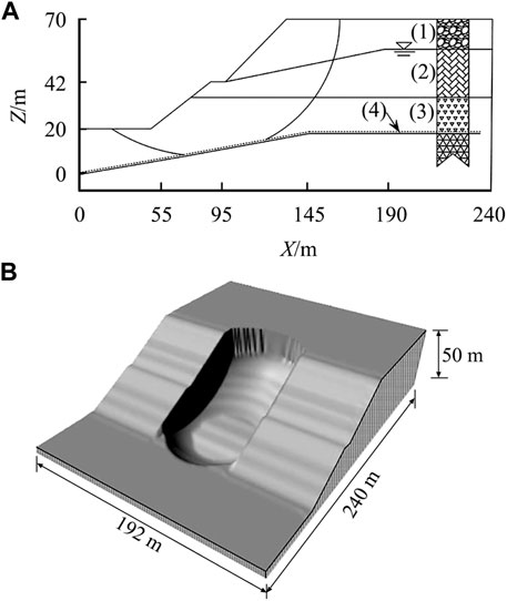
FIGURE 6. Slope example 2. (A) Cross section of slope, (B)The DEM model on the surface of the slope.
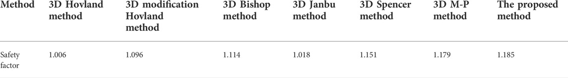
TABLE 2. Calculation results.
Analysis of the results from Table 2:
(1) The results of the 3D Hovland method, the 3D modification Hovland method, the 3D Bishop method, and the 3D Janbu method are smaller, followed by the results of the Spencer method. The M-P method and the proposed method have the largest calculation results, and the results obtained by the strict method are the largest, followed by the quasi-strict method, and the non-strict method is the smallest.
(2) According to the calculation result, the rationality of the approximation function, that is, the calculation result of the proposed method, is close to the real value;
(3) The result of the proposed method is 2.7% different from the quasi-strict method (three-dimensional Spencer method), and 6% different from that of the non-strict method (three-dimensional Bishop method), which is like Deng Dong’s (Deng and Liang, 2017). The difference obtained by equality is close, which verifies the correctness of the calculation result of the proposed method to be close to the strict method.
GIS can provide a unified platform for complex and multi-source data, and all target-related data can be converted into GIS raster datasets based on columnar raster cells. Based on the GIS platform, combined with its advantages in processing complex spatial data, the limit equilibrium method can be easily extended to 3D (Carter, 1994).
For complex slope engineering problems, the factors affecting the three-dimensional stability evaluation mainly include topography, strata, geotechnical parameters, and groundwater. Due to the multi-source and complexity of these data, it is difficult to express these spatial data in the general slope stability analysis system, and GIS can provide a unified platform to process these complex spatial data.
By adding professional models to GIS, a three-dimensional slope stability analysis model based on grid-column units can be established to analyze the stability of three-dimensional slopes. The model has the advantages of simple data processing and easy programming.
If the distribution pattern of the normal stress on the sliding surface has a significant influence on the stability factor, the stability factor obtained by assuming the normal stress distribution on the sliding surface is unreasonable. Therefore, it is necessary to develop a discussion of the sensitivity of the stability factor to the normal stress distribution of the sliding surface.
Lu et al. (2012) studied the influence of the two-dimensional stability factor under different assumptions of normal stress on the sliding surface through calculation examples. The research results show that the error of the two-dimensional stability factor values obtained from different normal stresses on the sliding surface is small, but the distribution curves of the normal stress on the sliding surface are completely inconsistent. It can also be concluded that the influence of the normal stress distribution on the sliding surface on the two-dimensional stability factor is not significant.
In the three-dimensional state, the influence of different sliding surface normal stress distributions on the stability factor will be greatly increased, which requires constructing a reasonable sliding surface normal stress distribution. In this paper, by analyzing the composition of the normal stress of the sliding surface, an approximation function σ(x, y) of the normal stress distribution of the sliding surface of the symmetrical slope is constructed, and the approximation function is closer to the distribution function in the strict method. In this way, from the mathematical aspect, the problem that the normal stress of the sliding surface of the symmetrical slope has a significant influence on the stability factor is solved.
GIS is widely used in geotechnical engineering due to its advantages in data processing and analysis capabilities. For example, GIS can not only establish the stability analysis model of a single slope, but also can establish a large-scale regional slope stability analysis model. Compared with the traditional slope stability analysis software, GIS has inherent advantages (Irigaray et al., 2003).
The advantage of the proposed method is that a reasonable three-dimensional sliding surface normal stress assumption model is constructed based on GIS, which provides a theoretical calculation basis for establishing the limit equilibrium method based on the sliding surface normal stress assumption in GIS; secondly, the approximation function constructed in this paper overcomes the influence of large error on the slope stability factor in the three-dimensional state, and makes the calculation result closer to the real value.
(1) Using the spatial data analysis ability of GIS, a GIS model of limit equilibrium for three-dimensional slope stability analysis was established, and the limit equilibrium equation for solving the three-dimensional stability factor was deduced according to the limit equilibrium conditions. Using this model, the limit equilibrium method based on the assumption of normal stress on the sliding surface can be established in GIS, and it has the advantages of simple data processing and easy programming.
(2) Under the assumption of no force, the composition of the normal stress distribution of the sliding surface based on the grid column unit is deduced and analyzed, and it is concluded that in the composition of the normal stress
(3) For the normal stress distribution σ(x, y) along the sliding direction of the slide body, since the proportion of σ2(x) is rather small in the normal stress σ(x) on the sliding surface, and it is a continuous and approximately smooth curve, it can be considered to use a third-order Lagrangian polynomial. Due to the small proportion of σ2(x), the approximation function has little effect on the result, making the normal stress of the sliding surface more approximate to the distribution function in the strict method.
(4) For the entire sliding surface, considering the normal stress distribution σ(x) and σ(y), the approximation function σ(x, y) of the normal stress distribution of the sliding surface for any grid-column element of the slope can be obtained. The approximation function not only overcomes the influence of large error on the slope stability factor in the three-dimensional state, but also provides a theoretical calculation basis for establishing a three-dimensional symmetrical slope limit equilibrium method based on the assumption of normal stress on the sliding surface in GIS. The rationality of the approximation function is verified by an example.
(5) Through the verification of the case, the results calculated by the method in this paper are close to the results calculated by the strict method, which verifies that the assumed model of the normal stress of the sliding surface proposed in this paper is closer to the real value.
The original contributions presented in the study are included in the article/supplementary material, further inquiries can be directed to the corresponding author.
GY was responsible for the ideas of the article. LB and CW was responsible for the implementation of the algorithm. AF was responsible for checking the language.
I would like to express my sincere gratitude to LB, CW, and AF for their motivation and for providing me access to their immense knowledge during this research work.
Author LB was employed by China Coal Technology and Engineering Group Nanjing Design and Research Institute Co., Ltd.
The remaining authors declare that the research was conducted in the absence of any commercial or financial relationships that could be construed as a potential conflict of interest.
All claims expressed in this article are solely those of the authors and do not necessarily represent those of their affiliated organizations, or those of the publisher, the editors and the reviewers. Any product that may be evaluated in this article, or claim that may be made by its manufacturer, is not guaranteed or endorsed by the publisher.
Ayalew, L., and Yamagishi, H. (2005). The application of GIS-based logistic regression for landslide susceptibility mapping in the Kakuda-Yahiko Mountains, Central Japan. Geomorphology 65 (1/2), 15–31. doi:10.1016/j.geomorph.2004.06.010
Bell, J. M. (1968). General slope stability analysis. J. Soil Mech. Found. Div. 94 (SM6), 1253–1270. doi:10.1061/JSFEAQ.0001196
Carter, B. (1994). Geographic information systems for geoscientists: Modelling with GIS. United States: Pergamon.
Chen, C. F., and Zhu, J. F. (2010). A three-dimensional slope stability analysis procedure based on Morgenstern-Price method. Chin. J. Rock Mech. Eng. 29 (7), 1473–1480. doi:10.3969/j.issn.1000-6915.2013.01.016
Cheng, Y. M., and Yip, C. J. (200720071544). Three-dimensional asymmetrical slope stability analysis extension of bishop's, janbu's, and morgenstern–price's techniques. J. Geotech. Geoenviron. Eng. 133133 (12), 154412–161555. doi:10.1061/(asce)1090-0241(2007)133:12(1544)
Deng, D. P., and Liang, L. (2017). Three-dimensional limit equilibrium method for slope stability based on assumption of stress on slip surface. Rock Soil Mech. 38 (1), 189–196. doi:10.16285/j.rsm.2017.01.024
Du, Y., Lu, Y. D., Xie, M., Jia, J. L., Cong, X. M., and Wu, Y. Q. (20202020). Stability evaluation of creeping landslide considering variation of initial conditions. Chin. J. Rock Mech. Eng. 39 (S1), 2828–2836. doi:10.13722/j.cnki.jrme.2019.1079
Du, Y., Xie, M., Jiang, Y., Chen, C., Jia, B., and Huo, L. (2021). Review on the formation mechanism and early warning of rock collapse. Metal. Mine 50 (01), 106–119. doi:10.19614/j.cnki.jsks.202101008
Du, Y., Xie, M., Wu, Z. X., Liu, Q. Q., and He, Z. (20192019). Genetic mechanism about translational landslide and its safety evaluation. Chin. J. Rock Mech. Eng. 38 (S1), 2871–2880. doi:10.13722/j.cnki.jrme.2018.1251
Hovland, H. J. (1979). Closure to “three-dimensional slope stability analysis method”. J. Geotech. Engrg. Div. 105 (GT5), 693–695. doi:10.1061/ajgeb6.0000806
Hungr, O. (1987). An extension of Bishop's simplified method of slope stability analysis to three dimensions. Geotechnique 37 (1), 113–117. doi:10.1680/geot.1987.37.1.113
Irigaray, C., Fernández, T., and Chacón, J. (2003). Preliminary rock-slope-susceptibility assessment using GIS and the SMR classification. Nat. Hazards 30 (3), 309–324. doi:10.1023/B:NHAZ.0000007178.44617.c6
Leshchinsky, D. (19901990851). Slope stability analysis: Generalized approach. J. Geotech. Engrg. 116116 (5), 8515–8867. doi:10.1061/(asce)0733-9410(1990)116:5(851)
Low, B. K., and Wilson, H. T. (1997). Probabilistic slope analysis using Janbu's generalized procedure of slices. Comput. Geotechnics 21 (2), 121–142. doi:10.1016/S0266-352X(97)00019-0
Lu, K. L., Zhu, D, Y., and Yang, Y. (2012). Selection of constitution and distribution model of normal stresses over slip surface of slope. Rock Soil Mech. 33 (12), 3741–3746.
Xie, M., Esaki, T., and Cai, M. (2006b). GIS-based implementation of three-dimensional limit equilibrium approach of slope stability. J. Geotech. Geoenviron. Eng. 132 (5), 656–660. doi:10.1061/(asce)1090-0241(2006)132:5(656)
Xie, M., Esaki, T., Cheng, Q., and Wang, C. (2006a). Geographical information system-based computational implementation and application of spatial three-dimensional slope stability analysis. Comput. Geotechnics 33 (4), 260–274. doi:10.1016/j.compgeo.2006.07.003
Xie, M., Esaki, T., Zhou, G., and Mitani, Y. (200320031109). Geographic information systems-based three-dimensional critical slope stability analysis and landslide hazard assessment. J. Geotech. Geoenviron. Eng. 129129 (12), 110912–111118. doi:10.1061/(asce)1090-0241(2003)129:12(1109)
Yang, M. C. (2004). Explicit solution to safety factor for general slice method. Rock Soil Mech. 25 (Suppl. 2), 568–573. doi:10.3969/j.issn.1000-7598.2004.z2.120
Yu, G., Xie, M. W., Zheng, Z. Q., Qin, S. H., and Du, Y. (2019). Research on slope stability calculation method based on GIS. Rock Soil Mech. 40 (4), 1397–1404. doi:10.16285/j.rsm.2018.0540
Zheng, H., and Tham, L. G. (2010). Improved Bell’s method for the stability analysis of slopes. Int. J. Numer. Anal. Methods Geomech. 33 (14), 1673–1689. doi:10.1002/nag.794
Zhou, G., Esaki, T., Mitani, Y., and Mori, J. (2003). Spatial probabilistic modeling of slope failure using an integrated GIS Monte Carlo simulation approach. Eng. Geol. 68 (3-4), 373–386. doi:10.1016/S0013-7952(02)00241-7
Zhou, X. P., and Cheng, H. (2013). Analysis of stability of three-dimensional slopes using the rigorous limit equilibrium method. Eng. Geol. 160 (27), 21–33. doi:10.1016/j.enggeo.2013.03.027
Zhu, D. Y., and Lee, C. F. (2002). Explicit limit equilibrium solution for slope stability. Int. J. Numer. Anal. Methods Geomech. 26 (15), 1573–1590. doi:10.1002/nag.260
Zhu, D. Y., Lee, C. F., Jiang, H. D., and Kang, J. W. (2004). Solution of slope safety factor by modifying normal stresses over slip surface. Chin. J. Rock Mech. Eng. 23 (16), 2788–2791. doi:10.3321/j.issn:1000-6915.2004.16.023
Keywords: 3D slope, limit equilibrium, sliding surface normal stress, GIS, grid units
Citation: Yu G, Bu L, Wang C and Farooq A (2022) Composition analysis and distributed assumption GIS model of normal stress on the slope sliding surface. Front. Earth Sci. 10:923620. doi: 10.3389/feart.2022.923620
Received: 19 April 2022; Accepted: 29 June 2022;
Published: 25 July 2022.
Edited by:
Yan Du, University of Science and Technology Beijing, ChinaReviewed by:
Jingshu Xu, Beijing University of Technology, ChinaCopyright © 2022 Yu, Bu, Wang and Farooq. This is an open-access article distributed under the terms of the Creative Commons Attribution License (CC BY). The use, distribution or reproduction in other forums is permitted, provided the original author(s) and the copyright owner(s) are credited and that the original publication in this journal is cited, in accordance with accepted academic practice. No use, distribution or reproduction is permitted which does not comply with these terms.
*Correspondence: Guo Yu, NTQ3ODQ4NTg0QHFxLmNvbQ==
Disclaimer: All claims expressed in this article are solely those of the authors and do not necessarily represent those of their affiliated organizations, or those of the publisher, the editors and the reviewers. Any product that may be evaluated in this article or claim that may be made by its manufacturer is not guaranteed or endorsed by the publisher.
Research integrity at Frontiers
Learn more about the work of our research integrity team to safeguard the quality of each article we publish.