Quantitative Evaluation of Reservoir Heterogeneity in the Ordos Basin Based on Tamura Texture Features

The low permeability sandstone reservoir in the Ordos Basin displays heterogeneity with sedimentation and tectonic origins, which is mainly manifest by interbedding of sandstone and mudstone, bedding, and fractures (). There is a clear difference between this type of heterogeneity and pore heterogeneity and diagenetic heterogeneity. At present, academia pays less attention to this kind of heterogeneity and lacks a quantitative evaluation method. The imaging log can describe this kind of heterogeneity directly. The Tamura texture features (TTF) method was used to calculate the roughness of different heterogeneous intervals. It is found that the fracture has the largest roughness, followed by the oblique bedding and the horizontal bedding section, and the massive bedding has the smallest roughness. The GR curve roughness calculated by EMD is consistent with that calculated by TTF. Therefore, TTF can be used to quantitatively evaluate the heterogeneity of low permeability sandstone reservoirs based on the imaging log when the imaging log has the same size. The roughness of the imaging log calculated by the TTF method has a strong coupling with the sedimentary cycle. This method is accurate, objective, and easy to understand. This is another important application of TTF in addition to quantitative evaluation of the heterogeneity of low permeability sandstone reservoirs.

Introduction

Low permeability sandstone is defined as having overburden permeability less than or equal to 1 × 10⁻³ μm² (Newman, 1999; Yin and Wu, 2020). Globally, Low permeability sandstone reservoirs are increasingly becoming targets for petroleum exploration and development because they contain vast resources which were stranded before the advent of modern well completion technologies (e.g., hydraulic fracturing) (Panja et al., 2016; Yin et al., 2018; Chen J. et al., 2019; Li L. et al., 2020; Arzhilovsky et al., 2021; Liu et al., 2022). The Ordos basin contains some of the most widely distributed low permeability sandstone reservoirs in China, within which the Yangchang Formation is representative. In 2019, CNPC (China National Petroleum Corporation) announced the discovery of the billion-ton Qingcheng Oil Field within the Ch-7 oil generation layer (an oil layer of the Yanchang Formation) of the Ordos Basin, which confirmed the presence of low permeability sandstone reservoirs (Fu et al., 2020).

The Yangchang Formation in the Ordos Basin is a continental reservoir. The most unique feature of this type of petroleum system is the close association of source rocks and reservoirs to the point where they are indistinguishable; these low permeability sandstone reservoirs are extremely heterogeneous (Gong et al., 2021). To date, research on the heterogeneity of low permeability sandstone reservoirs has mainly focused on two aspects: 1) diagenetic heterogeneity (Liu et al., 2016; Cui et al., 2019; Sole et al., 2019; Li M. et al., 2020; Xie et al., 2020; Xiong et al., 2020; Yıldız and Yılmaz, 2020); and, 2) pore heterogeneity (Kadkhodaie-Ilkhchi et al., 2019; Nazari et al., 2019; Yang et al., 2020; Yin et al., 2020; Wang et al., 2021; Wang et al., 2022). This paper will focus on heterogeneity derived from sedimentation and tectonic controls, which is seldom discussed in the literature on low permeability sandstone reservoirs. There are three manifestations of this kind of heterogeneity, bedding, sand and mud interstratification, and fracture. The importance of sedimentary and tectonic derived heterogeneity in terms of its influence on physical and mechanical properties in low permeability sandstone reservoirs was most recently investigated by Liu et al. (2018). Using rock mechanical analysis, they found that subtle differences of mineralogical components within low permeability sandstone cause heterogeneous rock mechanical properties which ultimately control fracture initiation and propagation. Huang et al. (2018) noticed widespread development of the lamina in low permeability sandstones within the Ordos Basin. Their results showed that sand lamina in the low permeability sandstones significantly increases the TOC of the reservoir. Therefore, they suggested that the development of sandy laminas is the direct cause of the reservoir physical properties heterogeneity in low permeability sandstone.

Several different methods for quantitative evaluation of heterogeneity derived from sedimentation and tectonic controls have been developed. Yang et al. (2019) set up a neural network to evaluate the interbedding of low permeability sandstones in the southern Ordos Basin and used them to quantify vertical heterogeneity parameters in each layer. By calculating Lorentz Coefficients of gamma-ray logs, Yue (Yue et al., 2015) quantitatively evaluated the intraformational heterogeneity of low permeability sandstone and summarized the vertical sand body distribution pattern of the formation. Xiao (Xiao et al., 2019a) put forward a method for quantitative evaluation of the heterogeneity of low permeability sandstone reservoirs based on combining the rescaled range method and modal decomposition method and obtaining the mathematical relationship between the heterogeneity of reservoirs and oil production.

Logging curves are commonly considered to be the most efficient and accurate method of quantitatively evaluating reservoir heterogeneity (Raeesi et al., 2012; Amoura et al., 2019; Yarmohammadi et al., 2020). However, most methods focus on using conventional types of logs (i.e., gamma, resistivity, sonic, density, etc), while image log data is mostly ignored even though it can directly reflect the sedimentary characteristics of reservoirs. Image logs record changes in resistivity or acoustic velocity caused by fractures, caving, bedding, and so on, and these changes are displayed using different colored images designed to intuitively describe the characteristics of the formation. At present, image logs are assessed qualitatively with the naked eye which means that interpretations are subjective. There is an important need for quantitative parameters that can be widely used in image log analysis that will improve standardization and normalization of interpretive results.

Sedimentary strata are recognized as objects with self-similar characteristics, so the imaging log that records formation changes must be a global pattern with repeated local sub-patterns. Therefore, it is theoretically feasible to use texture analysis to extract characteristic parameters from image log data. This paper will use Tamura theory to calculate the roughness, contrast, and direction of heterogeneity captured by image logs. The mapping relationship between the roughness of imaging logs and the heterogeneity of low permeability sandstone is established, and the application of Tamura theory in the division of sedimentary cycles is assessed.

Geological Setting

The Ordos Basin, located in western China, is a large-scale cratonic superimposed basin that developed during the Mesozoic (Figure 1A). The basin is characterized by weak structural deformation, multicycle tectonic evolution and many rock types characterizing sedimentary environments (Chen Y. et al., 2019; Gong et al., 2019). This study focuses on the southwestern part of the Ordos Basin, where the Upper Triassic Yanchang Formation is an important oil-producing interval (Figure 1B). The reservoir intervals comprise parts of deltaic and shallow lacustrine systems, with continuous sedimentation and stable structure. Figure 1C is a typical lithological section of the Yanchang Formation in the southern Ordos Basin. It can be seen from the figure that the lithology of the target layer is mainly siltstone and argillaceous fine sandstone, which contains thin mudstone interlayers. The interbeds of sand and mud in the Yanchang Formation are frequent and have strong heterogeneity. The study area is located in the interior of the basin, so there is no surface exposure to the target interval. However, the Yanchang Formation crops out along the edge of the Ordos Basin.

FIGURE 1

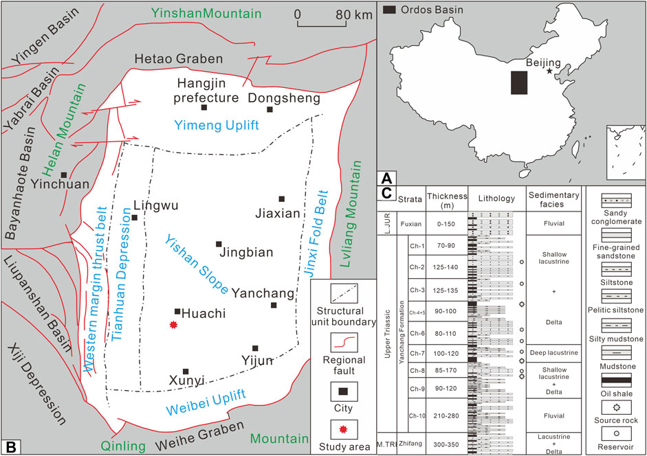
FIGURE 1. (A) Geographicmap of the Ordos Basin; (B) Location of the Ordos Basin in China; (C) Stratigraphic characteristics of the Yanchang Formation (Wang et al., 2020).

The profile observation shows that the Yangchang Formation in Ordos Basin is approximately horizontally distributed, with few large sedimentary structures such as folds and faults (Figure 2). But many small sedimentary structures can be observed, mainly including parallel bedding, oblique bedding, impression, and mud gravel. The vertical heterogeneity of the formation is very strong, which mainly shows that it is difficult to see a whole set of sandstone with a thickness of more than 5 m, and the formation is mostly a structure of thick sandstone with thin mudstone.

FIGURE 2

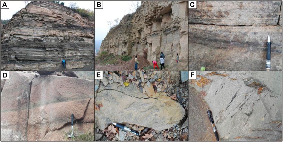
FIGURE 2. Profile photos of Yangchang formation in Ordos Basin. (A) Sand-mud interlayer in Ch-7 formation, located in Xunyi; (B) Mudstone interlayer in Ch-6 Formation, located in Xunyi; (C) Parallel bedding in Ch-7 Formation, located in Yanchang; (D) Oblique bedding in Ch-6 Formation, located in Jiaxian; (E) Impression in Ch-7 Formation, located in Yijun; (F) Mud gravel in Ch-6 Formation, located in Lingwu.

Small sedimentary structures are also observed in cores (Figure 3). There is mainly oblique bedding, parallel bedding, massive bedding, convoluted bedding, mud gravel, and fractures. The profile and core data show that the low permeability sandstone reservoir in the study area is characterized by frequent sand mud interbed, bedding and fractures. This feature directly results in a very strong reservoir heterogeneity, which affects the physical and mechanical properties of the reservoir (Zeng et al., 2022).

FIGURE 3

FIGURE 3. Core photos of Yangchang formation in study area. (A) Cross bedding; (B) Massive bedding; (C) Parallel bedding; (D) Convoluted bedding; (E) Oblique bedding; (F) Fractures; (G) Mud gravel; (H) Muddy strip; (I) Scratch.

Theory and Methodology

Texture refers to the local patterns that appear repeatedly in the image and their arrangement rules, reflecting the law of grayscale changes in the macro sense (Coggins and Jain, 1985). Although textures are ubiquitous in digital images, there is currently no formal texture definition (Lin et al., 2003). However, texture analysis has been applied to graphic analysis in various industries, such as medicine, remote sensing, photography, and other industries (Hashim et al., 2018; Delibas and Arslan, 2020). Based on the human visual perception test, Tamura proposed physical quantities to describe the texture features, namely: coarseness, contrast, directionality, linearity, regularity, and roughness (Tamura et al., 1975). The three most important parameters are coarseness, contrast, and directionality (Castelli and Bergman, 2002).

Coarseness

Roughness is a parameter that reflects the granularity in the texture and is the most basic texture feature. When the sizes of the two texture patterns are different, the patterns with larger sizes are coarser. The calculation of roughness can be divided into the following steps:

1) Calculate the average intensity of pixels in the active window with the size of $2^k\times 2^k$ pixels in the image:

$a_k\left(i,j\right)={\displaystyle {\sum }_{i\prime =i-2^{k-1}}^{i+2^{k-1}-1}{\displaystyle {\sum }_{j\prime =j-2^{k-1}}^{j+2^{k-1}-1}\frac{p\left(i\prime ,j\prime \right)}{2^{2k}}}},(1)$

Where, $p\left(i^{\text{'}},j^{\text{'}}\right)$ is the gray value of the pixel at $\left(i\prime ,j\prime \right)$.

2) For each pixel, calculate the average intensity difference between windows that do not overlap each other in the horizontal and vertical directions:

$E_{k,h}\left(i,j\right)=\left|a_k\left(i+2^{k-1},j\right)-a_k\left(i-2^{k-1},j\right)\right|,(2)$

$E_{k,v}\left(i,j\right)=\left|a_k\left(i,j+2^{k-1}\right)-a_k\left(i,j-2^{k-1}\right)\right|,(3)$

Where, for each pixel, there is a $k_{\max }$ The max value makes the $E$ value the maximum, using this $k_{max}$ is the best size:

$S_{best}\left(i,j\right)=2^{k_{max}}.(4)$

3) By calculating the average value of $S_{best}$ in the whole image to roughness:

$F_{crs}=\frac{1}{m\times n}{\displaystyle {\sum }_m^{i=1}{\displaystyle {\sum }_n^{j=1}{S}_{best}\left(i,j\right)}}.(5)$

Contrast

The contrast is obtained by the statistics of the pixel intensity distribution. The contrast is determined by four factors: dynamic range of gray level, polarization degree of the black and white part on the histogram, edge sharpness, and period of repetition pattern. In general, contrast refers to the first two factors. The calculation formula is as follows:

${\alpha }_4=\frac{{\mu }_4}{{\sigma }^4},(6)$

$F_{con}=\frac{\sigma }{{\alpha }_4^{1/4}},(7)$

Where, ${\mu }_4$ The fourth interval of the image is used to measure the steepness of the gray density function near the gray mean. ${\sigma }^2$ is the image variance.

Directionality

Directivity is the global characteristic of texture region, which describes how the texture diverges or concentrates in some directions. The calculation steps are as follows:

1) Calculate the gradient vector for each pixel:

${\Delta }_h={\displaystyle {\sum }_{k\in \left(-\mathrm{1,0,1}\right)}p\left(i+1,j+k\right)-p\left(i-1,j+k\right)},(8)$

${\Delta }_v={\displaystyle {\sum }_{k\in \left(-\mathrm{1,0,1}\right)}p\left(i+k,j+1\right)-p\left(i+k,j-1\right)}.(9)$

2) Calculate the magnitude $\Delta G$ and the local edge direction $\theta$:

$\left|\Delta G\right|=\left(\left|{\Delta }_h\right|+\left|{\Delta }_v\right|\right)/2,(10)$

$\theta ={\tanh }^{-1}\left(\frac{{\Delta }_h}{{\Delta }_v}\right)+\frac{\pi }{2}.(11)$

3) Discretize $\theta$, and use the histogram to count the number $H_D\left(\text{k}\right)$ of pixels in each $\theta$ where $\left|\Delta G\right|$ is greater than a given threshold

$H_D\left(\text{k}\right)=\frac{N_{\theta }\left(k\right)}{{{\displaystyle \sum }}_{i=0}^{n-1}{N}_{\theta }\left(i\right)},k=0, 1, \dots , n-1,(12)$

Where, $N_{\theta }\left(k\right)$ is the number of points at which $\left(2k-1\right)\pi /2n\le \theta <\left(2k+1\right)/2n$ and $\left|\Delta G\right|$ > t.

4) The directivity can be obtained by calculating the sharpness of the peaks. in the histogram. The method used is that if it is determined that there are multiple peaks, the second moments of the two valleys of the peak are added. This measure can be defined as follows:

$F_{dir}=1-r.n_p.{\displaystyle {\sum }_p^{n_p}{\displaystyle {\sum }_{\varphi \in w_p}{\left(\varphi -{\varphi }_p\right)}^2.H_D\left(\varphi \right)}},(13)$

Where $n_p$ is the number of peaks, ${\varphi }_p$ is $p$ th peak position of $H_D$, $w_p$ is the range of $p$ th peak between valleys, $r$ is the normalizing factor related to quantizing levels of $\varphi$, $\varphi$ is quantized direction code (cyclically in modulo 180°).

Feasibility of Texture Analysis of Imaging Log

Texture analysis is the process of extracting texture feature parameters through image processing technology, to obtain a quantitative or qualitative description of the texture. In addition to certain directivity and periodicity, the image used for texture analysis also needs to have very high-frequency information to extract accurate texture features.

Imaging logging map is quite different from maps in the fields of medicine, photography, remote sensing, and so on. It is the continuous monitoring of formation by resistivity detection brush. Generally, six brushes are set in the sampling process of the imaging logging map, and the brushes are separated from each other. Therefore, the final resistivity image is the resistivity trace with blank intervals in the transverse direction. In the imaging log, will the periodic 6 blank intervals change the directivity and periodicity of the original image? Will it create more high-frequency information that is difficult to distinguish? Given this, this study will set up two experiments to verify the feasibility of texture analysis of imaging logging.

Periodicity and Directivity of Imaging Log

Take an imaging log map in the study area as an example. The resolution of the log map is 482 × 482, the stratum thickness is 4 m. A group of gray data is randomly selected in the horizontal and vertical directions of the image to draw the gray curve, and then the box dimension method is used to calculate the fractal dimension of the two gray curves. The calculation method of the box dimension of the one-dimensional curve is not repeated here. For details, see references (Zaitouny et al., 2020).

The calculation flow of fractal dimensions in different directions of the imaging logging map is shown in Figure 4. Finally, the horizontal fractal dimension is 1.08 and the vertical fractal dimension is 1.31. It shows that the horizontal periodicity of the imaging log is very strong, and the texture is very simple. It can be seen from the horizontal gray distribution map that the horizontal gray presents extremely strong periodic characteristics, which is caused by six blank intervals in the imaging logging map. In the vertical direction, there is no blank interval, and it is difficult to observe the obvious periodicity of gray distribution. However, the linear fitting degree of the vertical box dimension is very good, which reflects that the imaging log map is also a fractal pattern in the vertical direction.

FIGURE 4

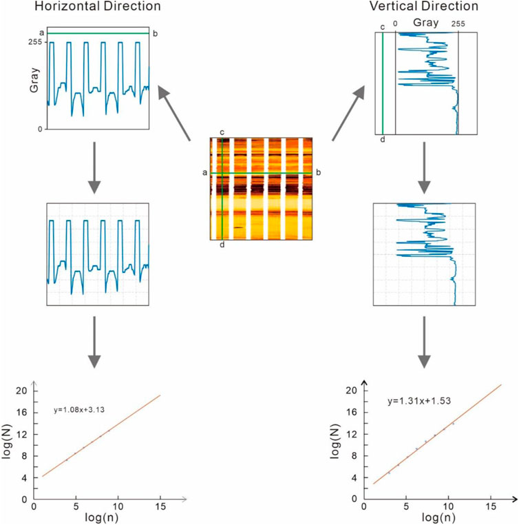
FIGURE 4. Calculation flow of fractal box dimension in different directions of imaging logging map.

Of course, the length of the imaging log map used in Figure 4 is short, and the distribution of six blank intervals is regular. However, in practice, the six blank intervals in the imaging log map will gradually change the position and extension angle with the increase of depth. When this happens, will it reduce the periodicity of the imaging log map? The author calculates the fractal dimension in different directions by selecting the 110 m imaging logging of the whole well section of Ch-7 member of the Yanchang formation. The results obtained are shown in Figure 5.

FIGURE 5

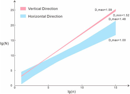
FIGURE 5. Characteristics of vertical and horizontal fractal curves of imaging log.

It can be found that the vertical fractal dimension is between 1.52 and 1.59 and the horizontal fractal dimension is between 1.00 and 1.48. Even if affected by six blank intervals, the vertical fractal characteristics of the imaging log are more stable. Horizontally, the fractal dimension of the imaging log is affected by 6 blank intervals, and the variation range is large.

Therefore, it can be determined that the blank intervals in the imaging log map do affect the periodicity in the horizontal direction of the imaging log to some extent, but the vertical imaging log map has stronger fractal characteristics, and its periodicity is mainly controlled by the light and dark changes of the imaging log itself, which has little to do with the blank intervals Figure 6

FIGURE 6

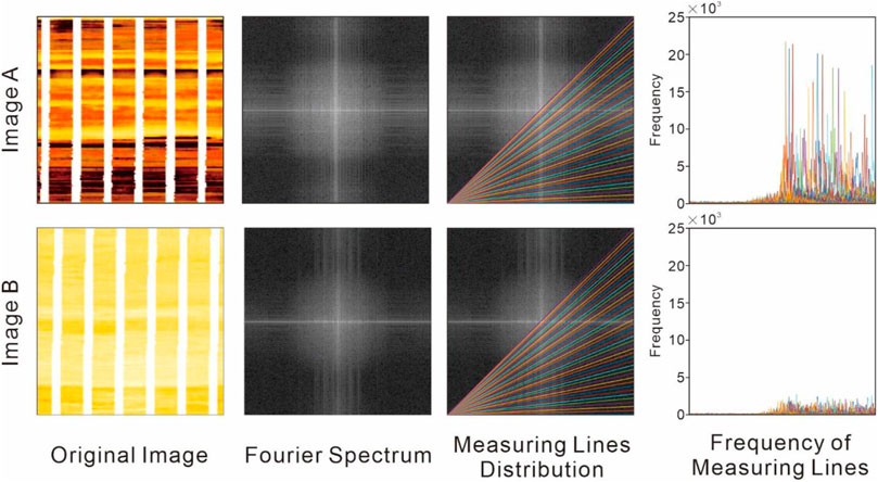
FIGURE 6. Frequency analysis of different types of imaging log.

High-Frequency Characteristics of Imaging Log

Generally, texture features are closely related to the high-frequency components in the image spectrum. Only when the image contains enough high-frequency information, the result of image texture analysis can be more accurate. Smoother images (mainly including low-frequency components) are generally not treated as texture images.

Therefore, to analyze the texture of the imaging log map, the imaging log map must contain enough high-frequency information. However, the frequent occurrence of six blank intervals in the imaging logging map causes the pixel mutation of the image, which directly leads to the increase of high-frequency information in the imaging logging map. Therefore, we designed the following experiments to determine whether the six blank intervals in the imaging log will weaken the high-frequency information caused by resistivity transformation.

Firstly, two imaging logging maps (Image A and Image B) with developed and undeveloped stratigraphic bedding are screened. Then Fourier transform the two images to obtain the Fourier spectrum. The white stripes in the Fourier spectrum are high-frequency information. It can be found that the high-frequency information in the spectrum of Image a is more than that of Image B. In order to more intuitively compare the frequency distribution characteristics of the two images, the frequency distribution on 0–45° of the two images is represented by the polar coordinate method. It is found that the frequencies of Image A and Image B are almost 10 times different in value.

Image B is the imaging logging map of homogeneous formation. It can be found from the map that the change of image fringe is moderate and the high frequency is not very prominent. Image A is an imaging log of heterogeneous formation. The image contains many dark stripes, resulting in extremely prominent high-frequency information, which is much larger than low-frequency information. Both images contain similar white intervals, but the changes of light and dark stripes caused by the heterogeneity of the formation itself will cause higher and more high-frequency information than the white intervals in the imaging logging map. It also shows that texture analysis is completely feasible for the analysis of imaging logging maps.

Data and Results

In the imaging log map of well A, four types of main developed heterogeneity layers in the study area are selected: oblique bedding, massive bedding, parallel bedding, and fracture layers. The representative imaging log map is selected for each heterogeneous type, and to facilitate the unified calculation of data, try to ensure that the size of each image is the same. According to this screening standard, the unified calculation standard is the stratum thickness of 10 m. Based on the data of resistivity imaging and diameter logging of well A, six images are selected for each type of heterogeneity, and a total of 24 images are obtained (Figures 7, 8).

FIGURE 7

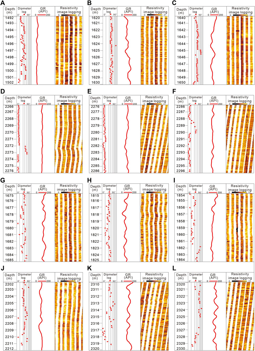
FIGURE 7. Resistivity imaging logging map of different heterogeneous intervals. (A–F): Parallel bedding; (G–L): Oblique bedding.

FIGURE 8

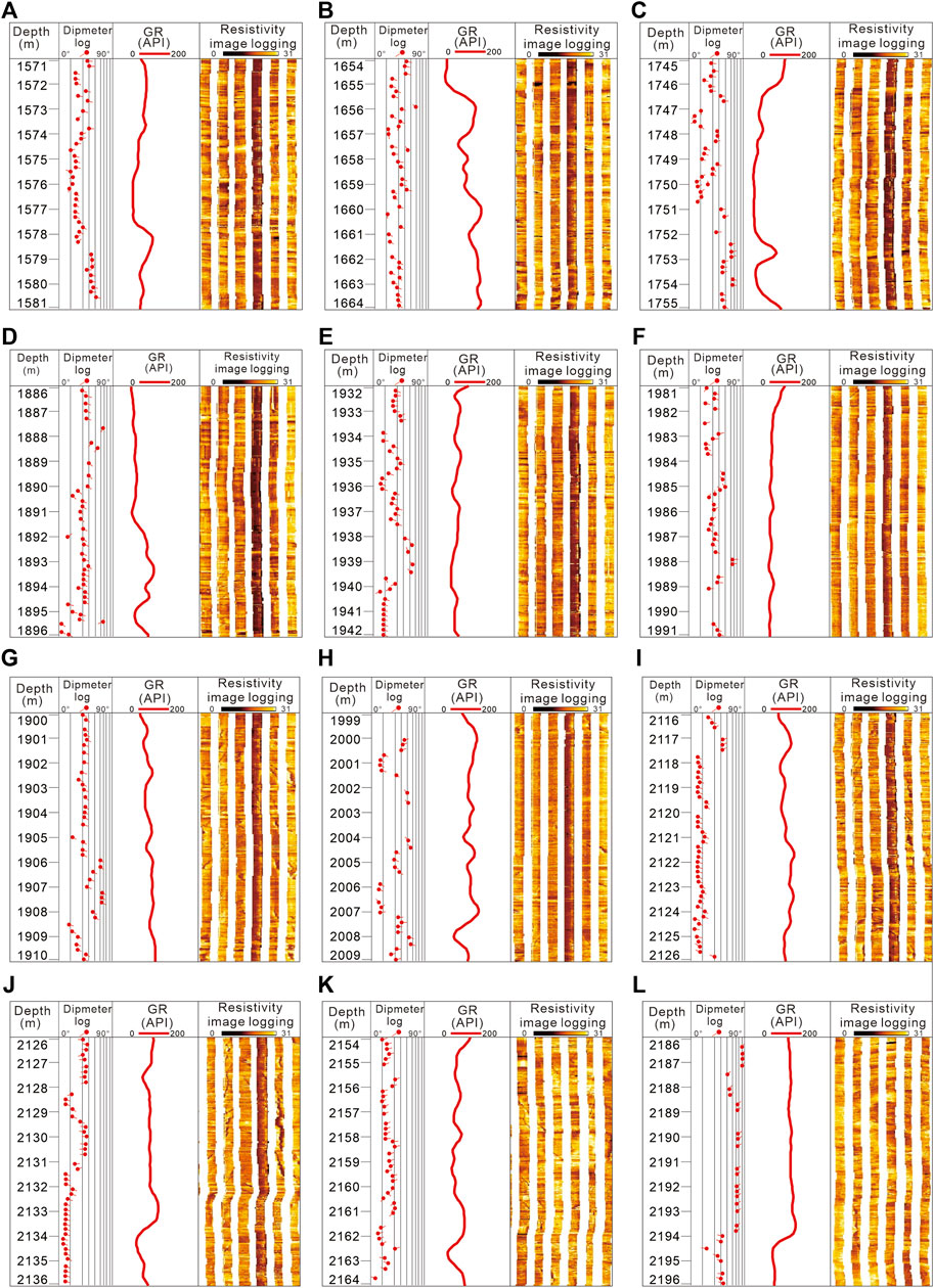
FIGURE 8. Resistivity imaging logging map of different heterogeneous intervals. (A–F): Massive bedding; (G–L): Fracture.

The roughness, contrast, and directivity of these 24 logging images are calculated by the Tamura texture features method (TTF), and the results are shown in Table 1. After normalizing the calculation results of the three parameters, draw a ternary diagram (Figure 9). It can be seen from the figure that the four types of heterogeneity are partitioned on the ternary map. Therefore, it can be concluded that it is feasible to quantitatively evaluate the formation heterogeneity based on TTF Method, and the specific evaluation effect needs to be further explored.

TABLE 1

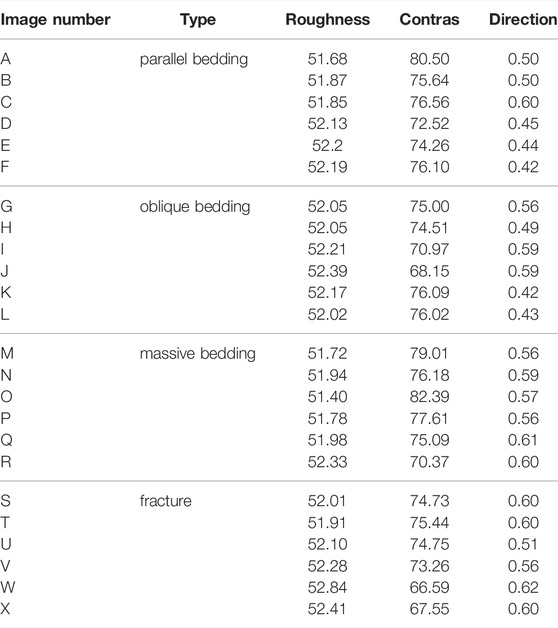
TABLE 1. Calculation results of roughness, contrast and directionality of imaging well logs of 4 types of heterogeneous intervals in well A.

FIGURE 9

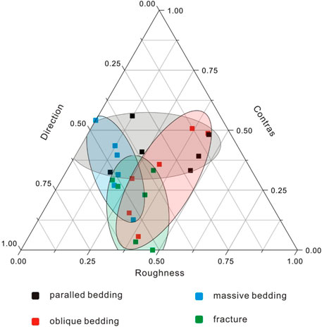
FIGURE 9. Ternary graph of roughness, contrast and directivity.

Discussion

Quantitative Evaluation of Reservoir Heterogeneity Based on Tamura Texture Features Method

Conventional logging curves reflect the inherent characteristics of a series of sedimentary strata such as lithology, electricity, and porosity. In the measurement process, the logging tool detects the characteristics of the formation with a fixed sampling frequency (one data is recorded every 0.25 m) and records information with the depth as the scale. Therefore, in essence, a conventional logging curve is a one-dimensional time series with self-similarity (Xiao et al. 2019b). Due to the time series characteristics of the logging curve, the roughness of the logging curve can be calculated. Compare the roughness of the imaging log with the roughness of the conventional logging curve. If the two roughness is linearly related, it shows that the TTF can quantitatively reflect the formation heterogeneity.

At present, empirical mode decomposition (EMD) is commonly used to calculate the roughness of the logging curve (Subhakar and Chandrasekhar, 2016; Xiao et al. 2019). EMD method was proposed by Norden E. Huang et al., in 1998 (Huang et al., 1998). This method is based on the time scale characteristics of the data itself to decompose the signal, without any pre-set basis function. It has a very obvious advantage in dealing with non-stationary and non-linear data (Martins et al., 2016).

Figure 10 shows the calculation process of the EMD method, which can be divided into three steps:

(1) The maximum and minimum points of the original data $X\left(t\right)$ are fitted by the cubic spline difference function to form the upper $U_j\left(t\right)$ and lower $L_j\left(t\right)$ envelope lines of the original data, and the average envelope function is calculated:

$m_j\left(t\right)=\frac{U_j\left(t\right)+L_j\left(t\right)}{2}.(14)$

(2) Subtracting the average envelope line data $m_j\left(t\right)$ from the original data $X\left(t\right)$ to obtain a new data series $H_j\left(t\right)$. Judge whether $H_j\left(t\right)$ meets the conditions of the IMF. If it does, the next step will be taken. Otherwise, perform the first two operations on $H_j\left(t\right)$ until $H_j\left(t\right)$ meets the conditions of the IMF;

(3) If the filtering process is completed successfully, the first IMF_j is achieved. Subtract IMF_j from the original data and repeat the above process to get the next IMF_j+1. Until the residual R(t) is a single point signal or only one base point exists.

FIGURE 10

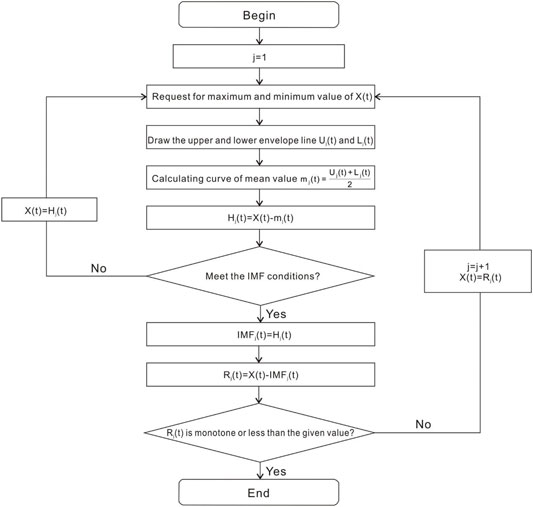
FIGURE 10. Calculating flow of EMD method.

Finally, the original signal is expressed as:

$X\left(t\right)={\displaystyle {\sum }_{j=1}^{n}IM{F}_j\left(t\right)+R\left(t\right)},(15)$

Where, n is the total number of IMF obtained by EMD decomposition of the original signal.

At present, most scholars (Flandrin et al., 2004; Azadeh et al., 2013; Gaci and Zaourar, 2014) regard EMD as a second-order filter in the wavenumber domain. Therefore, for a given signal, its average wave number $k_m$ is inversely proportional to the IMF number m:

$k_m=k{\rho }^{-m},(16)$

Where, k is a constant, ρ can be obtained by fitting the linear relationship between m and log($k_m$). Since EMD signals according to the time scale characteristics of the data, it is found that ρ is related to the EMD scale. When ρ is high, the corresponding characteristic scale is low, and vice versa. Therefore, ρ can be used to quantitatively judge the complexity of the original signal. Previous researchers (Gairola, 2017) obtained the relationship between ρ and the formation lithology heterogeneity, that is, the lower the ρ value, the more complex the lithologic unit.

GR logging curve can reflect the shale content in the formation precisely and has good feedback for the heterogeneity characteristics in the formation. Therefore, the heterogeneity of the natural gamma curve (GR) corresponding to 24 imaging logs can be calculated by the EMD method. Then, the box type map which can reflect the distribution of original data is used to compare the formation heterogeneity calculated by the two methods (Figure 11).

FIGURE 11

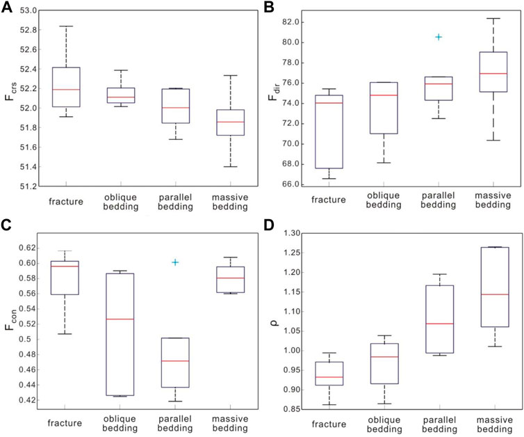
FIGURE 11. Comparison between TTF analysis results and EMD analysis results. (A) Roughness of image log; (B) Directivity of image log; (C) contrast of image log; (D) Roughness of GR curve.

The results show that the ρ value of the GR curve is the largest in massive bedding, followed by parallel bedding and oblique bedding, and the smallest in fracture layer. Because the ρ value is inversely proportional to the heterogeneity of the stratum, the order of the heterogeneity of the GR curve corresponding to the four types of heterogeneity is fracture development section, fracture bedding, parallel bedding, and massive bedding. Among them, the heterogeneity of fracture layer is the largest, and that of massive bedding is the smallest. This result has the same relationship with the roughness of the imaging log calculated by the TTF. However, the other two important parameters of TTF, directionality, and contrast, have little correlation with the heterogeneity coefficient calculated by the EMD.

Based on the knowledge gained above, it can be determined that TTF can quantitatively evaluate reservoir heterogeneity based on the imaging log data. The premise is that the selected imaging log should have the same size to ensure that the calculated roughness is comparable.

The Coupling Relationship Between Tamura Texture Roughness and Sedimentary Cycle

The GR curve can sensitively reflect the change in mud content, and an important role in sedimentology is to divide the sedimentary cycles. However, this method is too subjective. Especially when dividing the strata with more sedimentary cycles, different scholars have different sedimentary cycles. The TTF method can calculate the image roughness of the imaging log to quantitatively evaluate the formation heterogeneity. If the roughness of a continuous imaging log is calculated at a fixed scale, a set of data that can reflect the vertical heterogeneity of the formation can be obtained. This set of data contains various types of heterogeneous information in the stratum, and lithological changes are one of them. Therefore, the TTF method can be further explored, that is, whether the sedimentation cycle can be divided by the roughness of the imaging log image.

Select 1,600–2060 m formation of Well A in the research area as the research stratum (Figure 12). The interval discussed in this paper includes Ch-2, Ch-3, Ch-4+5, and some Ch-6 formations. The sedimentary characteristics of these strata have been fully studied by scholars, and a sedimentary system recognized by the academic community has been established. A more reliable conclusion can be obtained by comparing the sedimentary cycle of this formation with the sedimentary cycle divided by the TTF. The three-level cycle in Figure 12 is a recognized division plan in academia, and the fourth-level cycle is divided by the author according to the actual situation of the study area.

FIGURE 12

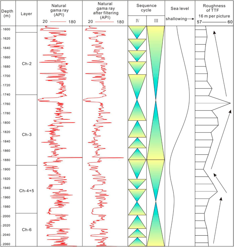
FIGURE 12. Comparison of TTF analysis results and sedimentary cycles at different scales. When the thickness of the formation is 16 m, the change trend of the roughness of the imaging log perfectly matches the change of sea level.

To avoid the noise interference of the logging curve, the selected GR curve is processed by a Gauss filter. In this section, two third-order sedimentary cycles can be identified from the bottom to the top. Based on the third-order sedimentary cycle, the fourth-order cycle can be further divided by analyzing the change of GR curve details. Similarly, sea-level changes can be plotted by the overall change of the GR curve.

The results show that the overall trend of image roughness perfectly matches the trend of sea-level change. And in some sequence boundary numbers, such as 1750, 1880, and 1965 m, the image roughness also shows extreme value.

Therefore, it can be concluded that the roughness of the imaging log based on the TTF method has a strong coupling with the sedimentary cycle of the formation. This conclusion undoubtedly confirms the right direction of this discussion. To verify and compare the accuracy of this method in sedimentary cycle division, it is necessary to find a mature method for comparative analysis. In this discussion, it is decided to adopt the continuous wavelet transform as the comparison method.

Continuous wavelet transform (CWT) is a continuous function of time for a decomposition, so that it becomes several wavelets. Mathematically, a function that is continuous-time and integrable $f\left(t\right)$ Can be expressed by the following integral:

$W_{\psi }\left(a,b\right)=\frac{1}{\sqrt{\left|a\right|}}\underset{-\infty }{\overset{+\infty }{{\displaystyle \int }}}f\left(t\right)\overline{\psi }\left(\frac{t-b}{a}\right)dt,(17)$

Where: $W_{\psi }$ is the wavelet coefficient, $a\times b$ matrix; $a$ is the scale factor, which indicates the scaling associated with the rating; $b$ is the time shift factor, which indicates the shift of the wavelet function; $f\left(t\right)$ is the signal data; $\psi$ is Wavelet basis function; $\overline{\psi }$ is the conjugate of the wavelet basis function.

The algorithm of CWT can be divided into four steps (Figure 13). It can be found that the correlation C can be obtained by analyzing the similarity between wavelet basis function and signal on different scales. The division of sedimentary cycles is to select the interval that best fits the sedimentology model at different scales. Both are to change the observation scale to extract the internal information of the time series (logging curve). This is the reason why continuous wavelet transform is widely used in the division of sedimentary cycles.

FIGURE 13

FIGURE 13. Flow chart of continuous wavelet transform (CWT) (Kadkhodaie, 2017).

When CWT is used to identify sedimentary cycles, the wavelet basis function should be selected first, and then the wavelet coefficient curve can be obtained by changing the scale of the wavelet basis function (Perez et al., 2013). By analyzing the change in the local energy group of the wavelet time-frequency energy spectrum and the periodic oscillation characteristics of the wavelet coefficient curve, the cyclicity of strata can be obtained. And then establish a corresponding relationship with sequence boundaries at all levels to achieve the purpose of dividing stratigraphic sedimentary cycles.

The analysis object is the GR logging curve of 1592–5064 m in well A. It can be seen from the previous analysis that the kind of wavelet basis function is the decisive factor for the accuracy of signal analysis when CWT is used to identify sedimentary cycles. Therefore, the Morlet wavelet, Haar wavelet, and Gaussian wavelet are the wavelet basis functions of CWT respectively (Figure 14). By comparing the energy map and wavelet coefficient map with the scale of 500, it is found that the local part of the energy map obtained by using the Morlet wavelet basis function is the best, and each energy cluster can be identified. In addition, the oscillation of its wavelet coefficient curve is also better than the others. Therefore, the GR curve is processed by CWT of the Morlet wavelet basis function.

FIGURE 14

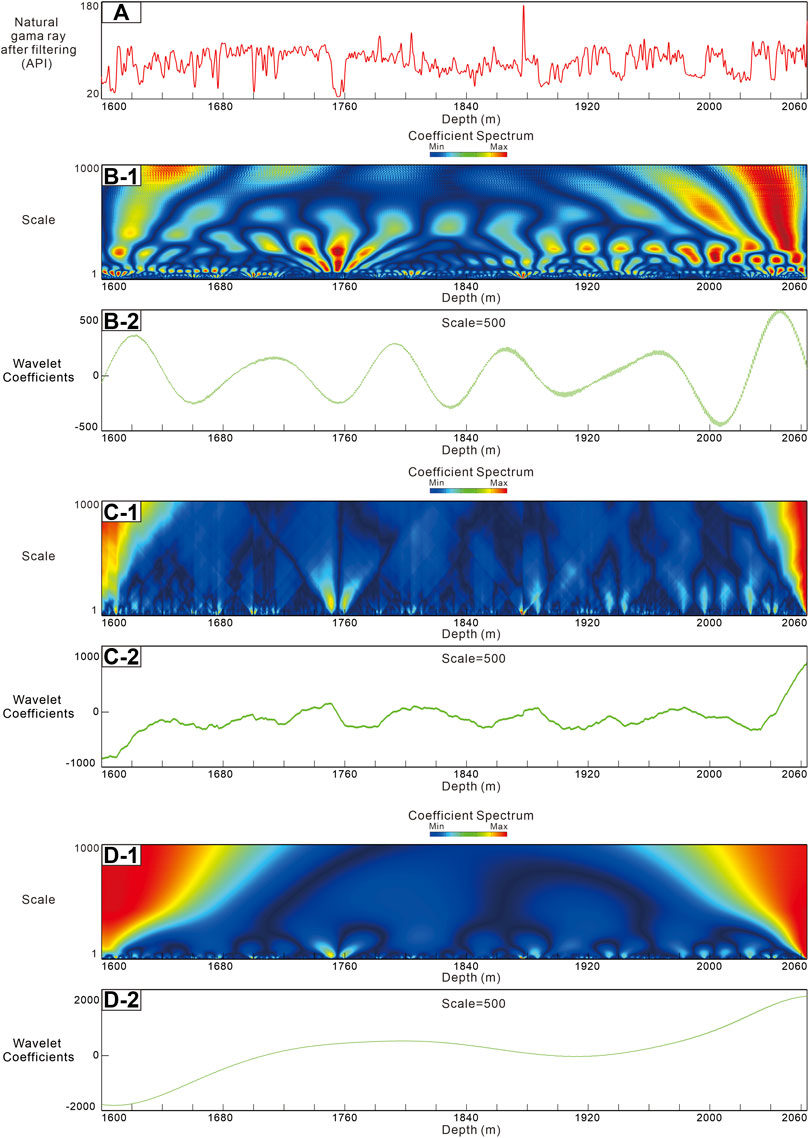
FIGURE 14. (A) GR curve; (B-1): Energy spectrum of CWT based on Morlet wavelet; (B-2): Wavelet coefficient curve of CWT based on Morlet wavelet; (C-1): Energy spectrum of CWT based on Haar wavelet; (C-2): Wavelet coefficient curve of CWT based on Haar wavelet; (D-1): Energy spectrum of CWT based on Gaussian wavelet; (D-2): Wavelet coefficient curve of CWT based on Gaussian wavelet.

Figure 15 shows the analysis results of the GR curve by CWT. By observing the distribution characteristics of local energy clusters on a wavelet energy spectrum with a time scale of 1,000, three levels of energy cluster distribution characteristics can be identified. They are small-scale 200–450, mesoscale 450–700, and large scale 700–1,000. According to these three scales, three levels of sedimentary cycles can be divided.

FIGURE 15

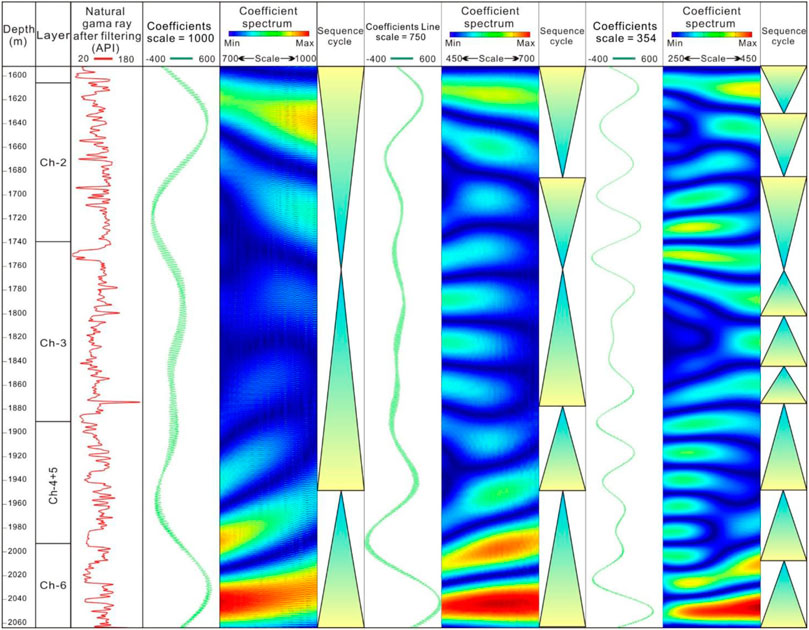
FIGURE 15. Recognition results of sedimentary cycle based on CWT method.

DWT can obtain different levels of sedimentary cycles by selecting different wavelet analysis scales, while TTF can make the data-dense by reducing the thickness of the analysis layer, thereby obtaining a smaller level of sedimentary cycles.

The Tamura texture roughness of imaging logging is obtained by using stratum thickness of 16, 8, and 4 m respectively. According to the obtained roughness curve, three sedimentary cycles in different scales are also divided. A comparison of the two sedimentary cycles is shown in Figure 16.

FIGURE 16

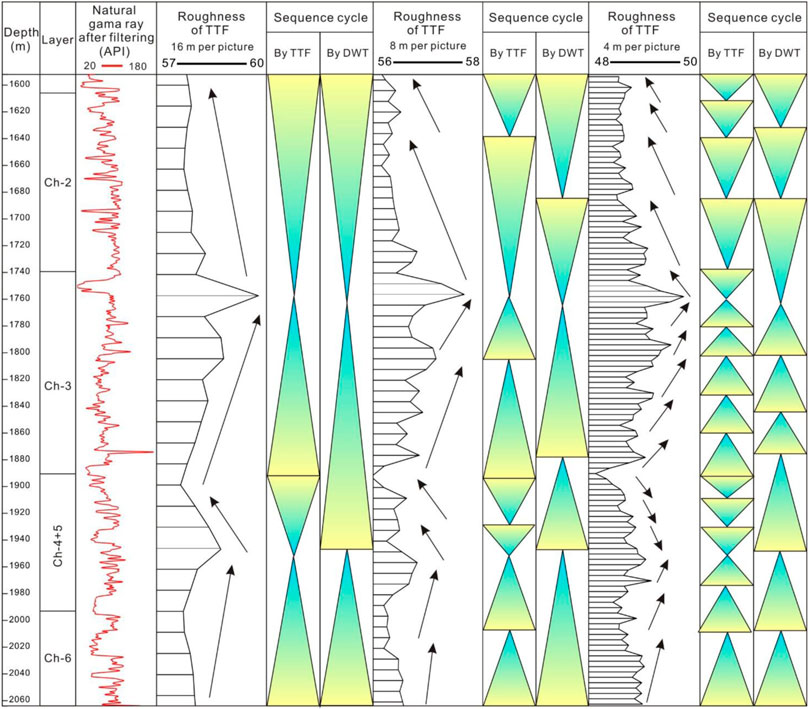
FIGURE 16. Comparison between TTF and CWT sedimentation cycle recognition results.

It can be seen from Figure 16 that there are two main features of sedimentary cycle division results of CWT and TTF. First of all, the large-scale sedimentary interfaces are the same, and the small-scale sedimentary cycle interfaces are different. Taking the 1760–1945 m stratum as an example, the continuous wavelet transform method identifies this stratum as a positive cycle with the change of stratum lithology from coarse to a fine from bottom to top. However, the TTF method divides 1760–1945 m into 1885–1945 m stratigraphic lithology reverse cycle and 1760–1885 m positive cycle. It can be seen from the GR curve that in the 1885–1945 m section, the GR curve is in the shape of a superimposed funnel, and there is a reverse cycle. Therefore, the interpretation of the latter is more reasonable.

Second, the small-scale sedimentary cycles identified by the TTF method are more precise. The principle of the TTF method to identify sedimentary cycles is to set a stratum thickness as the scale coefficient, calculate the Tamura roughness of the imaging log map on the scale, and identify sedimentary cycles by the change of roughness. The results obtained by this method are unique, accurate, and objective. CWT also needs to set a scale to identify sedimentary cycles, but compared with the former, the scale is the multi-solution, abstract and subjective. Therefore, the sedimentary cycles identified by the CWT method vary greatly and are not accurate relative to the TTF method.

Thirdly, the TTF method is more accurate to judge the cyclicity of sequence. The CWT sedimentary cycle recognition method is based on the distribution of local energy groups on the wavelet energy spectrum to divide the sequence. TTF method is to divide the sequence according to the roughness change of the imaging log. This method can see the precise numerical change from the roughness curve, so it can judge whether the sequence is a positive cycle or reverse cycle, to improve the reliability of sedimentary cycle division.

In a word, the TTF method is accurate, objective, and easy to understand in sedimentary cycle identification of low permeability sandstone reservoirs. This is another important application of TTF in addition to quantitative evaluation of the heterogeneity of low permeability sandstone reservoirs.

Conclusion

(1) The low permeability sandstone reservoir in the Ordos Basin has developed a kind of heterogeneity controlled by sedimentation and tectonic action, which is mainly manifested by a sand-mud interlayer, bedding, and fracture. There is a clear difference between this type of heterogeneity and pore heterogeneity and diagenetic heterogeneity;

(2) Resistivity imaging log is a kind of picture with periodicity, directivity, and rich high-frequency information. In the resistivity image, the white interval caused by data acquisition will not weaken the periodicity, directivity, and high-frequency information caused by the change of formation heterogeneity. Therefore, Therefore, the texture analysis of the imaging logging is completely feasible.

(3) The GR curve roughness calculated by EMD is consistent with that calculated by the TTF method. Therefore, the TTF method can be used to quantitatively evaluate the heterogeneity of low permeability sandstone reservoirs based on the imaging log when the imaging log has the same size.

(4) The reservoir heterogeneity coefficient calculated by the TTF method can be used to divide sedimentary cycles, and the accuracy is better than the wavelet transform method and manual identification method. Texture analysis of imaging logging is a new idea and method, and the division of sedimentary cycles is only one of its popularization and application. It is hoped that the reservoir heterogeneity evaluation method based on the TTF method can get more practical applications in the future.

Data Availability Statement

The original contributions presented in the study are included in the article/Supplementary Material, further inquiries can be directed to the corresponding author.

Author Contributions

ZX is responsible for the idea and writing of this article and WD, SH, ZW, CX, HG and XZ are responsible for the data interpretation.

Funding

This research was jointly funded by the National Institute of Natural Hazards, Ministry of Emergency Management of China (former Institute of Crustal Dynamics, China Earthquake Administration) Research Fund (ZDJ 2021-24), China Scholarship Council (201906400021), and Natural Science Foundation of Fujian Province (2019J05162).

Conflict of Interest

Author SH was employed by the company Yanchang Petroleum (Group) Co., Ltd. Author ZW was employed by the company Changqing Oilfield.

The remaining authors declare that the research was conducted in the absence of any commercial or financial relationships that could be construed as a potential conflict of interest.

Publisher’s Note

All claims expressed in this article are solely those of the authors and do not necessarily represent those of their affiliated organizations, or those of the publisher, the editors and the reviewers. Any product that may be evaluated in this article, or claim that may be made by its manufacturer, is not guaranteed or endorsed by the publisher.

Acknowledgments

The authors would like to thank the staff of all the laboratories that cooperated in performing the tests and analyses. The author would also like to thank the Department of Energy and Mineral Engineering of Penn State University for its support, which makes this visit possible.

References

Amoura, S., Gaci, S., Bounif, M. A., and Boussa, L. (2019). On Characterizing Heterogeneities from Velocity Logs Using Hölderian Regularity Analysis: A Case Study from Algerian Tight Devonian Reservoirs. J. Appl. Geophys. 170, 103833. doi:10.1016/j.jappgeo.2019.103833

CrossRef Full Text | Google Scholar

Arzhilovsky, A. V., Grischenko, A. S., Grischenko, A. S., Smirnov, D. S., Kornienko, S. A., Baisov, R. R., et al. (2021). A Case Study of Drilling Horizontal Wells with Multistage Hydraulic Fracturing in Low-Permeable Reservoirs of the Tyumen Formation at the Fields of RN-Uvatneftegas. OIJ 2021 (02), 74–76. doi:10.24887/0028-2448-2021-2-74-76

CrossRef Full Text | Google Scholar

Castelli, V., and Bergman, L. D. B. (2002). Image Databases: Search and Retrieval of Digital Imagery. New York: Wiley.

Google Scholar

Chen, J., Yao, J., Mao, Z., Li, Q., Luo, A., Deng, X., et al. (2019). Sedimentary and Diagenetic Controls on Reservoir Quality of Low-Porosity and Low-Permeability Sandstone Reservoirs in Chang101, Upper Triassic Yanchang Formation in the Shanbei Area, Ordos Basin, China. Mar. Petroleum Geol. 105, 204–221. doi:10.1016/j.marpetgeo.2019.04.027

CrossRef Full Text | Google Scholar

Chen, Y., Zhu, Z., and Zhang, L. (2019). Control Actions of Sedimentary Environments and Sedimentation Rates on Lacustrine Oil Shale Distribution, an Example of the Oil Shale in the Upper Triassic Yanchang Formation, Southeastern Ordos Basin (NW China). Mar. Petroleum Geol. 102, 508–520. doi:10.1016/j.marpetgeo.2019.01.006

CrossRef Full Text | Google Scholar

Coggins, J. M., and Jain, A. K. (1985). A Spatial Filtering Approach to Texture Analysis. Patt. Recognit. Lett. 3 (3), 195–203. doi:10.1016/0167-8655(85)90053-4

CrossRef Full Text | Google Scholar

Cui, J., Li, S., and Mao, Z. (2019). Oil-bearing Heterogeneity and Threshold of Tight Sandstone Reservoirs: A Case Study on Triassic Chang7 Member, Ordos Basin. Mar. Petroleum Geol. 104, 180–189. doi:10.1016/j.marpetgeo.2019.03.028

CrossRef Full Text | Google Scholar

Del Sole, L., Antonellini, M., and Calafato, A. (2020). Characterization of Sub-seismic Resolution Structural Diagenetic Heterogeneities in Porous Sandstones: Combining Ground-Penetrating Radar Profiles with Geomechanical and Petrophysical In Situ Measurements (Northern Apennines, Italy). Mar. Petroleum Geol. 117, 104375–104422. doi:10.1016/j.marpetgeo.2020.104375

CrossRef Full Text | Google Scholar

Delibaş, E., and Arslan, A. (2020). DNA Sequence Similarity Analysis Using Image Texture Analysis Based on First-Order Statistics. J. Mol. Graph. Model. 99, 107603–107611. doi:10.1016/j.jmgm.2020.107603

PubMed Abstract | CrossRef Full Text | Google Scholar

Flandrin, P., Rilling, G., and Goncalves, P. (2004). Empirical Mode Decomposition as a Filter Bank. IEEE Signal Process. Lett. 11, 112–114. doi:10.1109/LSP.2003.821662

CrossRef Full Text | Google Scholar

Fu, S., Fu, J., Niu, X., Li, S., Wu, Z., Zhou, X., et al. (2020). Reservoir Formation Conditions and Key Technologies for Exploration and Development in Qingcheng Large Oilfield. Petroleum Res. 5, 181–201. doi:10.1016/j.ptlrs.2020.06.002

CrossRef Full Text | Google Scholar

Gaci, S., and Zaourar, N. (2014). On Exploring Heterogeneities from Well Logs Using the Empirical Mode Decomposition. Energy Procedia 59, 44–50. doi:10.1016/j.egypro.2014.10.347

CrossRef Full Text | Google Scholar

Gairola, G. S., and Chandrasekhar, E. (2017). Heterogeneity Analysis of Geophysical Well-Log Data Using Hilbert-Huang Transform. Phys. A Stat. Mech. its Appl. 478, 131–142. doi:10.1016/j.physa.2017.02.029

CrossRef Full Text | Google Scholar

Gong, L., Fu, X., Wang, Z., Gao, S., Jabbari, H., Yue, W., et al. (2019). A New Approach for Characterization and Prediction of Natural Fracture Occurrence in Tight Oil Sandstones with Intense Anisotropy. Bulletin 103 (6), 1383–1400. doi:10.1306/12131818054

CrossRef Full Text | Google Scholar

Gong, L., Gao, S., Liu, B., Yang, J., Fu, X., Xiao, F., et al. (2021). Quantitative Prediction of Natural Fractures in Shale Oil Reservoirs. Geofluids 2021, 1–15. doi:10.1155/2021/5571855

CrossRef Full Text | Google Scholar

Hashim, N., Adebayo, S. E., Abdan, K., and Hanafi, M. (2018). Comparative Study of Transform-Based Image Texture Analysis for the Evaluation of Banana Quality Using an Optical Backscattering System. Postharvest Biol. Technol. 135, 38–50. doi:10.1016/j.postharvbio.2017.08.021

CrossRef Full Text | Google Scholar

Huang, H., Sun, W., Ji, W., Chen, L., Jiang, Z., Bai, Y., et al. (2018). Impact of Laminae on Gas Storage Capacity: A Case Study in Shanxi Formation, Xiasiwan Area, Ordos Basin, China. J. Nat. Gas Sci. Eng. 60, 92–102. doi:10.1016/j.jngse.2018.09.001

CrossRef Full Text | Google Scholar

Huang, N. E., Shen, Z., Long, S. R., Wu, M. C., Shih, H. H., Zheng, Q., et al. (1998). The Empirical Mode Decomposition and the Hilbert Spectrum for Nonlinear and Non-stationary Time Series Analysis. Proc. R. Soc. Lond. A 454, 903–995. doi:10.1098/rspa.1998.0193

CrossRef Full Text | Google Scholar

Kadkhodaie, A., and Rezaee, R. (2017). Intelligent Sequence Stratigraphy through a Wavelet-Based Decomposition of Well Log Data. J. Nat. Gas Sci. Eng. 40, 38–50. doi:10.1016/j.jngse.2017.02.010

CrossRef Full Text | Google Scholar

Kadkhodaie-Ilkhchi, R., Kadkhodaie, A., Rezaee, R., and Mehdipour, V. (2019). Unraveling the Reservoir Heterogeneity of the Tight Gas Sandstones Using the Porosity Conditioned Facies Modeling in the Whicher Range Field, Perth Basin, Western Australia. J. Petroleum Sci. Eng. 176, 97–115. doi:10.1016/j.petrol.2019.01.020

CrossRef Full Text | Google Scholar

Li, L., Zhang, X., and Deng, H. (2020). Mechanical Properties and Energy Evolution of Sandstone Subjected to Uniaxial Compression with Different Loading Rates. J. Min. Strata Control Eng. 2 (4), 043037. doi:10.13532/j.jmsce.cn10-1638/td.20200407.001

CrossRef Full Text | Google Scholar

Li, M., Guo, Y., Li, Z., and Wang, H. (2020). The Diagenetic Controls of the Reservoir Heterogeneity in the Tight Sand Gas Reservoirs of the Zizhou Area in China's East Ordos Basin: Implications for Reservoir Quality Predictions. Mar. Petroleum Geol. 112, 104088. doi:10.1016/j.marpetgeo.2019.104088

CrossRef Full Text | Google Scholar

Li, Y., Song, Y., Jiang, Z., Yin, L., Chen, M., and Liu, D. (2018). Major Factors Controlling Lamina Induced Fractures in the Upper Triassic Yanchang Formation Tight Oil Reservoir, Ordos Basin, China. J. Asian Earth Sci. 166, 107–119. doi:10.1016/j.jseaes.2018.07.040

CrossRef Full Text | Google Scholar

Lin, H.-C., Chiu, C.-Y., and Yang, S.-N. (2003). Finding Textures by Textual Descriptions, Visual Examples, and Relevance Feedbacks. Pattern Recognit. Lett. 24, 2255–2267. doi:10.1016/S0167-8655(03)00052-7

CrossRef Full Text | Google Scholar

Liu, J., Liu, K., and Huang, X. (2016). Effect of Sedimentary Heterogeneities on Hydrocarbon Accumulations in the Permian Shanxi Formation, Ordos Basin, China: Insight from an Integrated Stratigraphic Forward and Petroleum System Modelling. Mar. Petroleum Geol. 76, 412–431. doi:10.1016/j.marpetgeo.2016.05.028

CrossRef Full Text | Google Scholar

Liu, J., Yang, H., Xu, K., Wang, Z., Liu, X., Cui, L., et al. (2022). Genetic Mechanism of Transfer Zones in Rift Basins: Insights from Geomechanical Models. GSA Bull.. doi:10.1130/B36151.1

CrossRef Full Text | Google Scholar

Martins, L. G. N., Stefanello, M. B., Degrazia, G. A., Acevedo, O. C., Puhales, F. S., Demarco, G., et al. (2016). Employing the Hilbert-Huang Transform to Analyze Observed Natural Complex Signals: Calm Wind Meandering Cases. Phys. A Stat. Mech. its Appl. 462, 1189–1196. doi:10.1016/j.physa.2016.06.147

CrossRef Full Text | Google Scholar

Moghtaderi, A., Flandrin, P., and Borgnat, P. (2013). Trend Filtering via Empirical Mode Decompositions. Comput. Statistics Data Analysis 58, 114–126. doi:10.1016/j.csda.2011.05.015

CrossRef Full Text | Google Scholar

Nazari, M. H., Tavakoli, V., Rahimpour-Bonab, H., and Sharifi-Yazdi, M. (2019). Investigation of Factors Influencing Geological Heterogeneity in Tight Gas Carbonates, Permian Reservoir of the Persian Gulf. J. Petroleum Sci. Eng. 183, 106341–106418. doi:10.1016/j.petrol.2019.106341

CrossRef Full Text | Google Scholar

Newman, P. J. (1999). The Geology and Hydrocarbon Potential of the Peel and Solway Basins, East Irish Sea. J. Pet. Geol. 22, 305–324. doi:10.1111/j.1747-5457.1999.tb00989.x

CrossRef Full Text | Google Scholar

Panja, P., Conner, T., and Deo, M. (2016). Factors Controlling Production in Hydraulically Fractured Low Permeability Oil Reservoirs. Ijogct 13 (No. 1), 1–18. doi:10.1504/IJOGCT.2016.078033

CrossRef Full Text | Google Scholar

Perez-Muñoz, T., Velasco-Hernandez, J., and Hernandez-Martinez, E. (2013). Wavelet Transform Analysis for Lithological Characteristics Identification in Siliciclastic Oil Fields. J. Appl. Geophys. 98, 298–308. doi:10.1016/j.jappgeo.2013.09.010

CrossRef Full Text | Google Scholar

Raeesi, M., Moradzadeh, A., Ardejani, F. D., and Rahimi, M. (2012). Classification and Identification of Hydrocarbon Reservoir Lithofacies and Their Heterogeneity Using Seismic Attributes, Logs Data and Artificial Neural Networks. J. Petrol. Sci. Eng. 82–83, 151–165. doi:10.1016/j.petrol.2012.01.012

PubMed Abstract | CrossRef Full Text | Google Scholar

Subhakar, D., and Chandrasekhar, E. (2016). Reservoir Characterization Using Multifractal Detrended Fluctuation Analysis of Geophysical Well-Log Data. Phys. A Stat. Mech. its Appl. 445 (1), 57–65. doi:10.1016/j.physa.2015.10.103

CrossRef Full Text | Google Scholar

Tamura, H., Mori, S., and Yamawaki, T. (1978). Textural Features Corresponding to Visual Perception. IEEE Trans. Syst. Man. Cybern. 8, 460–473. doi:10.1109/TSMC.1978.4309999

CrossRef Full Text | Google Scholar

Wang, Y., Cheng, H., Hu, Q., Liu, L., Jia, L., Gao, S., et al. (2022). Pore Structure Heterogeneity of Wufeng-Longmaxi Shale, Sichuan Basin, China: Evidence from Gas Physisorption and Multifractal Geometries. J. Petroleum Sci. Eng. 208, 109313. doi:10.1016/j.petrol.2021.109313

CrossRef Full Text | Google Scholar

Wang, Y., Liu, L., and Cheng, H. (2021). Gas Adsorption Characterization of Pore Structure of Organic-Rich Shale: Insights into Contribution of Organic Matter to Shale Pore Network. Nat. Resour. Res. 30 (3), 2377–2395. doi:10.1007/s11053-021-09817-5

CrossRef Full Text | Google Scholar

Wang, Z., Luo, X., Lei, Y., Zhang, L., Shi, H., Lu, J., et al. (2020). Impact of Detrital Composition and Diagenesis on the Heterogeneity and Quality of Low-Permeability to Tight Sandstone Reservoirs: an Example of the Upper Triassic Yanchang Formation in Southeastern Ordos Basin. J. Petroleum Sci. Eng. 195, 107596. doi:10.1016/j.petrol.2020.107596

CrossRef Full Text | Google Scholar

Xiao, Z., Ding, W., Hao, S., Taleghani, A. D., Wang, X., Zhou, X., et al. (2019a). Quantitative Analysis of Tight Sandstone Reservoir Heterogeneity Based on Rescaled Range Analysis and Empirical Mode Decomposition: A Case Study of the Chang 7 Reservoir in the Dingbian Oilfield. J. Petroleum Sci. Eng. 182, 106326. doi:10.1016/j.petrol.2019.106326

CrossRef Full Text | Google Scholar

Xiao, Z., Ding, W., Liu, J., Tian, M., Yin, S., Zhou, X., et al. (2019b). A Fracture Identification Method for Low-Permeability Sandstone Based on R/S Analysis and the Finite Difference Method: A Case Study from the Chang 6 Reservoir in Huaqing Oilfield, Ordos Basin. J. Petroleum Sci. Eng. 174, 1169–1178. doi:10.1016/j.petrol.2018.12.017

CrossRef Full Text | Google Scholar

Xie, D., Yao, S., Cao, J., Hu, W., and Qin, Y. (2020). Origin of Calcite Cements and Their Impact on Reservoir Heterogeneity in the Triassic Yanchang Formation, Ordos Basin, China: A Combined Petrological and Geochemical Study. Mar. Petroleum Geol. 117, 104376. doi:10.1016/j.marpetgeo.2020.104376

CrossRef Full Text | Google Scholar

Xiong, Y., Tan, X., Dong, G., Wang, L., Ji, H., Liu, Y., et al. (2020). Diagenetic Differentiation in the Ordovician Majiagou Formation, Ordos Basin, China: Facies, Geochemical and Reservoir Heterogeneity Constraints. J. Petroleum Sci. Eng. 191, 107179. doi:10.1016/j.petrol.2020.107179

CrossRef Full Text | Google Scholar

Yang, S., Huang, X., Yin, C., Xu, Y., Zhao, Y., and Yan, J. (2019). Intra-layer Heterogeneity of Sandstone with Different Origins in Deep-Water Environment and its Causes. Sustain. Comput. Inf. Syst. 21, 10–18. doi:10.1016/j.suscom.2018.11.003

CrossRef Full Text | Google Scholar

Yang, W., Wang, Q., Wang, Y., Jiang, Z., Song, Y., Li, Y., et al. (2020). Pore Characteristic Responses to Categories of Depositional Microfacies of Delta-Lacustrine Tight Reservoirs in the Upper Triassic Yanchang Formation, Ordos Basin, NW China. Mar. Petroleum Geol. 118, 104423. doi:10.1016/j.marpetgeo.2020.104423

CrossRef Full Text | Google Scholar

Yarmohammadi, S., Kadkhodaie, A., and Hosseinzadeh, S. (2020). An Integrated Approach for Heterogeneity Analysis of Carbonate Reservoirs by Using Image Log Based Porosity Distributions, NMR T2 Curves, Velocity Deviation Log and Petrographic Studies: A Case Study from the South Pars Gas Field, Persian Gulf Basin. J. Petroleum Sci. Eng. 192, 107283. doi:10.1016/j.petrol.2020.107283

CrossRef Full Text | Google Scholar

Yıldız, G., and Yılmaz, İ. Ö. (2020). Reservoir Heterogeneity of Ordovician Sandstone Reservoir (Bedinan Formation, SE Turkey): Diagenetic and Sedimentological Approachs. Mar. Petroleum Geol. 118, 104444. doi:10.1016/j.marpetgeo.2020.104444

CrossRef Full Text | Google Scholar

Yin, S., Dong, L., Yang, X., and Wang, R. (2020). Experimental Investigation of the Petrophysical Properties, Minerals, Elements and Pore Structures in Tight Sandstones. J. Nat. Gas Sci. Eng. 76, 103189. doi:10.1016/j.jngse.2020.103189

CrossRef Full Text | Google Scholar

Yin, S., Lv., D,, and Ding, W. (2018). New Method for Assessing Microfracture Stress Sensitivity in Tight Sandstone Reservoirs Based on Acoustic Experiments. Int. J. Geomechanics 4, 1–16. doi:10.1061/(ASCE)GM.1943-5622.0001100

CrossRef Full Text | Google Scholar

Yin, S., and Wu, Z. (2020). Geomechanical Simulation of Low-Order Fracture of Tight Sandstone. Mar. Petroleum Geol. 117, 104359. doi:10.1016/j.marpetgeo.2020.104359

CrossRef Full Text | Google Scholar

Yue, C., Yang, X., Zhong, X., Pang, B., and Wang, F. (2015). Evaluation of Formation Heterogeneity Using Lorentz Coefficient of Logging Curves. J. Jilin Univ. Earth Sci. 45 (10), 1539–1546. doi:10.13278/j.cnki.jjuese

CrossRef Full Text | Google Scholar

Zaitouny, A., Small, M., Hill, J., Emelyanova, I., and Clennell, M. B. (2020). Fast Automatic Detection of Geological Boundaries from Multivariate Log Data Using Recurrence. Comput. Geosciences 135, 104362. doi:10.1016/j.cageo.2019.104362

CrossRef Full Text | Google Scholar

Zeng, L., Gong, L., Guan, C., Zhang, B., Wang, Q., Zeng, Q., et al. (2022). Natural Fractures and Their Contribution to Tight Gas Conglomerate Reservoirs: A Case Study in the Northwestern Sichuan Basin, China. J. Petroleum Sci. Eng. 210, 110028. doi:10.1016/j.petrol.2021.110028

CrossRef Full Text | Google Scholar